Quantum State Reconstruction From Incomplete Data

Abstract

Knowing and guessing, these are two essential epistemological pillars in the theory of quantum-mechanical measurement. As formulated quantum mechanics is a statistical theory. In general, a priori unknown states can be completely determined only when measurements on infinite ensembles of identically prepared quantum systems are performed. But how one can estimate (guess) quantum state when just incomplete data are available (known)? What is the most reliable estimation based on a given measured data? What is the optimal measurement providing only a finite number of identically prepared quantum objects are available? These are some of the questions we address in the article.

We present several schemes for a reconstruction of states of quantum systems from measured data:
(1) We show how the maximum entropy (MaxEnt) principle can be efficiently used for an estimation of quantum states (i.e. density operators or Wigner functions) on incomplete observation levels, when just a fraction of system observables are measured (i.e., the mean values of these observables are known from the measurement). With the extention of observation levels more reliable estimation of quantum states can be performed. In the limit, when all system observables (i.e., the quorum of observables) are measured, the MaxEnt principle leads to a complete reconstruction of quantum states, i.e. quantum states are uniquely determined. We analyze the reconstruction via the MaxEnt principle of bosonic systems (e.g. single-mode electromagnetic fields modeled as harmonic oscillators) as well as spin systems. We present results of MaxEnt reconstruction of Wigner functions of various nonclassical states of light in different observation levels. We also present results of numerical simulations which illustrate how the MaxEnt principle can be efficiently applied for a reconstruction of quantum states from incomplete tomographic data.
(2) When only a finite number of identically prepared systems are measured, then the measured data contain only information about frequencies of appearances of eigenstates of certain observables. We show that in this case states of quantum systems can be estimated with the help of quantum Bayesian inference. We analyze the connection between this reconstruction scheme and the reconstruction via the MaxEnt principle in the limit of infinite number of measurements. We discuss how an a priori knowledge about the state which is going to be reconstructed can be utilized in the estimation procedure. In particular, we discuss in detail the difference between the reconstruction of states which are a priori known to be pure or impure.
(3) We show how to construct the optimal generalized measurement of a finite number of identically prepared quantum systems which results in the estimation of a quantum state with the highest fidelity. We show how this optimal measurement can in principle be realized. We analyze two physically interesting examples - a reconstruction of states of a spin-1/2 and an estimation of phase shifts.

I INTRODUCTION: MEASUREMENT OF QUANTUM STATES

The concept of a quantum state represents one of the most fundamental pillars of the paradigm of quantum theory [1, 2, 3]. Contrary to its mathematical elegance and convenience in calculations, the physical interpretation of a quantum state is not so transparent. The problem is that the quantum state (described either by a state vector, or density operator or a phase-space probability density distribution) does not have a well defined objective status, i.e. a state vector is not an objective property of a particle. According to Peres (see [1], p. 374): “There is no physical evidence whatsoever that every physical system has at every instant a well defined state… In strict interpretation of quantum theory these mathematical symbols [i.e., state vectors] represent statistical information enabling us to compute the probabilities of occurrence of specific events.” Once this point of view is adopted then it becomes clear that any “measurement” or a reconstruction of a density operator (or its mathematical equivalent) can be understood exclusively as an expression of our knowledge about the quantum mechanical state based on a certain set of measured data. To be more specific, any quantum-mechanical reconstruction scheme is nothing more than an a posteriori estimation of the density operator of a quantum-mechanical (microscopic) system based on data obtained with the help of a macroscopic measurement apparatus [3]. The quality of the reconstruction depends on the “quality” of the measured data and the efficiency of the reconstruction procedure with the help of which the data analysis is performed. In particular, we can specify three different situations. Firstly, when all system observables are precisely measured. In this case the complete reconstruction of an initially unknown state can be performed (we will call this the reconstruction on the complete observation level). Secondly, when just part of the system observables is precisely measured then one cannot perform a complete reconstruction of the measured state. Nevertheless, the reconstructed density operator still uniquely determines mean values of the measured observables (we will denote this scheme as reconstruction on incomplete observation levels). Finally, when measurement does not provide us with sufficient information to specify the exact mean values (or probability distributions) but only the frequencies of appearances of eigenstates of the measured observables, then one can perform an estimation (e.g. reconstruction based on quantum Bayesian inference) which is the “best” with respect to the given measured data and the a priori knowledge about the state of the measured system.

A Complete observation level

Providing all system observables (i.e., the quorum [4, 5]) have been precisely measured, then the density operator of a quantum-mechanical system can be completely reconstructed (i.e., the density operator can be uniquely determined based on the available data). In principle, we can consider two different schemes for reconstruction of the density operator (or, equivalently, the Wigner function) of the given quantum-mechanical system. The difference between these two schemes is based on the way in which information about the quantum-mechanical system is obtained. The first type of measurement is such that on each element of the ensemble of the measured states only a single observable is measured. In the second type of measurement a simultaneous measurement of conjugate observables is assumed. We note that in both cases we will assume ideal, i.e., unit-efficiency, measurements.

1 Quantum tomography

When the single-observable measurement is performed, a distribution $w_{|\Psi\rangle}(A)$ for a particular observable $\hat{A}$ of the state $|\psi\rangle$ is obtained in an unbiased way [6], i.e., $w_{|\Psi\rangle}(A)=|\langle\Phi_{A}|\Psi\rangle|^{2}$, where $|\Phi_{A}\rangle$ are eigenstates of the observable $\hat{A}$ such that $\sum_{A}|\Phi_{A}\rangle\langle\Phi_{A}|=\hat{1}$. Here a question arises: What is the smallest number of distributions $w_{|\Psi\rangle}(A)$ required to determine the state uniquely? If we consider the reconstruction of the state of a harmonic oscillator, then this question is directly related to the so-called Pauli problem [7] of the reconstruction of the wave-function from distributions $w_{|\Psi\rangle}(q)$ and $w_{|\Psi\rangle}(p)$ for the position and momentum of the state $|\Psi\rangle$. As shown by Gale, Guth and Trammel [8] the knowledge of $w_{|\Psi\rangle}(q)$ and $w_{|\Psi\rangle}(p)$ is not in general sufficient for a complete reconstruction of the wave (or, equivalently, the Wigner) function. In contrast, one can consider an infinite set of distributions $w_{|\Psi\rangle}(x_{\theta},\theta)$ of the rotated quadrature $\hat{x}_{\theta}=\hat{q}\cos\theta+\hat{p}\sin\theta$. Each distribution $w_{|\Psi\rangle}(x_{\theta},\theta)$ can be obtained from a measurement of a single observable $\hat{x}_{\theta}$, in which case a detector (filter) is prepared in an eigenstate $|x_{\theta}\rangle$ of this observable. It has been shown by Vogel and Risken [9] that from an infinite set (in the case of the harmonic oscillator) of the measured distributions $w_{|\Psi\rangle}(x_{\theta},\theta)$ for all values of $\theta$ such that $[0<\theta\leq\pi]$, the Wigner function can be reconstructed uniquely via the inverse Radon transformation. In other words knowledge of the set of distributions $w_{|\Psi\rangle}(x_{\theta},\theta)$ is equivalent to knowledge of the Wigner function. This scheme for reconstruction of the Wigner function (i.e., the optical homodyne tomography) has recently been realized experimentally by Raymer and his coworkers [10, 11]. In these experiments the Wigner functions of a coherent state and a squeezed vacuum state have been reconstructed from tomographic data. Very comprehensive discussion of the quantum homodyne tomography can be found in the book by Leonhardt [12] and the review article by Welsch, Vogel and Opatrný [13]. Quantum homodyne tomography can be efficiently performed not only with the help of the inverse Radon transformation but also with the help of the so-called pattern functions [14, 15]. Other theoretical concept of Wigner-function reconstruction has been considered by Royer [16].

Quantum-state tomography can be applied not only to optical fields but also for reconstruction of other physical systems. In particular, recently Janicke and Wilkens [17] have suggested that Wigner functions of atomic waves can be tomographically reconstructed. Kurtsiefer et al. [18] have performed experiments in which Wigner functions of matter wave packets have been reconstructed. Yet another example of the tomographic reconstruction is a reconstruction of Wigner functions of vibrational states of trapped atomic ions theoretically described by a number of groups [19] and experimentally measured by Leibfried et al. [20]. Vibrational motional states of molecules have also been reconstructed by this kind of quantum tomography by Dunn et al. [21].

Leonhardt [22] has recently developed a theory of quantum tomography of discrete Wigner functions describing states of quantum systems with finite-dimensional Hilbert spaces (for instance, angular momentum or spin). We note that the problem of reconstruction of states of finite-dimensional systems is closely related to various aspects of quantum information processing, such as reading of registers of quantum computers [23]. This problem also emerges when states of atoms are reconstructed (see, for instance, [24]).

Here we stress once again, that reconstruction on the complete observation level (such as quantum tomography) is a deterministic inversion procedure which helps us to “rewrite” measured data in the more convenient form of a density operator or a Wigner function of the measured state.

2 Filtering with quantum rulers

For the case of simultaneous measurement of two non-commuting observables (let us say $\hat{q}$ and $\hat{p}$), it is not possible to construct a joint eigenstate of these two operators, and therefore it is inevitable that the simultaneous measurement of two non-commuting observables introduces additional noise (of quantum origin) into measured data. This noise is associated with Heisenberg’s uncertainty relation and it results in a specific “smoothing” (equivalent to a reduction of resolution) of the original Wigner function of the system under consideration (see [25] and [26] and the reviews [27, 28]). To describe the process of simultaneous measurement of two non-commuting observables, Wódkiewicz [29] has proposed a formalism based on an operational probability density distribution which explicitly takes into account the action of the measurement device modeled as a “filter” (quantum ruler). A particular choice of the state of the ruler samples a specific type of accessible information concerning the system, i.e., information about the system is biased by the filtering process The quantum-mechanical noise induced by filtering formally results in a smoothing of the original Wigner function of the measured state [25, 26], so that the operational probability density distribution can be expressed as a convolution of the original Wigner function and the Wigner function of the filter state. In particular, if the filter is considered to be in its vacuum state then the corresponding operational probability density distributions is equal to the Husimi ($Q$) function [25]. The $Q$ function of optical fields has been experimentally measured using such an approach by Walker and Carroll [32]. The direct experimental measurement of the operational probability density distribution with the filter in an arbitrary state is feasible in an 8-port experimental setup of the type used by Noh, Fougéres and Mandel [33] (see also [34, 12]).

As a consequence of a simultaneous measurement of non-commuting observables the measured distributions are fuzzy (i.e., they are equal to smoothed Wigner functions). Nevertheless, if detectors used in the experiment have unit efficiency (in the case of an ideal measurement), the noise induced by quantum filtering can be “separated” from the measured data and the density operator (Wigner function) of the measured system can be “extracted” from the operational probability density distribution. In particular, the Wigner function can be uniquely reconstructed from the $Q$ function (for more details see [35]). This extraction procedure is technically quite involved and it suffers significantly if additional stochastic noise due to imperfect measurement is present in the data.

We note that propensities, and in particular $Q$-functions, can also be associated with discrete phase space and they can in principle be measured directly [36]. These discrete probability distributions contain complete information about density operators of measured systems. Consequently, these density operators can be uniquely determined from the discrete-phase space propensities.

B Reduced observation levels and MaxEnt principle

As we have already indicated it is well understood that density operators (or Wigner functions) can, in principle, be uniquely reconstructed using either the single observable measurements (optical homodyne tomography) or the simultaneous measurement of two non-commuting observables. The completely reconstructed density operator (or, equivalently, the Wigner function) contains information about all independent moments of the system operators. For example, in the case of the quantum harmonic oscillator, the knowledge of the Wigner function is equivalent to the knowledge of all moments $\langle(\hat{a}^{\dagger})^{m}\hat{a}^{n}\rangle$ of the creation $(\hat{a}^{\dagger})$ and annihilation $(\hat{a})$ operators.

In many cases it turns out that the state of a harmonic oscillator is characterized by an infinite number of independent moments $\langle(\hat{a}^{\dagger})^{m}\hat{a}^{n}\rangle$ (for all $m$ and $n$). Analogously, the state of a quantum system in a finite-dimensional Hilbert space can be characterized by a very large number of independent parameters. A complete measurement of these moments may take an infinite time to perform. This means that even though the Wigner function can in principle be reconstructed the collection of a complete set of experimental data points is (in principle) a never ending process. In addition the data processing and numerical reconstruction of the Wigner function are time consuming. Therefore experimental realization of the reconstruction of the density operators (or Wigner functions) for many systems can be difficult.

In practice, it is possible to measure just a finite number of independent moments of the system operators, so that only a subset $\hat{G}_{\nu}$ ($\nu=1,2,...,n)$ of observables from the quorum (this subset constitutes the so-called observation level [37]) is measured. In this case, when the complete information about the system is not available, one needs an additional criterion which would help to reconstruct (or estimate) the density operator uniquely. Provided mean values of all observables on the given observation level are measured precisely, then the density operator (or the Wigner function) of the system under consideration can be reconstructed with the help of the Jaynes principle of maximum entropy (the so called MaxEnt principle) [37] (see also [38, 39, 40]). The MaxEnt principle provides us with a very efficient prescription to reconstruct density operators of quantum-mechanical systems providing the mean values of a given set of observables are known. It works perfectly well for systems with infinite Hilbert spaces (such as the quantum-mechanical harmonic oscillator) as well as for systems with finite-dimensional Hilbert spaces (such as spin systems). If the observation level is composed of the quorum of the observables (i.e., the complete observation level), then the MaxEnt principle represents an alternative to quantum tomography, i.e. both schemes are equally suitable for the analysis of the tomographic data (for details see [41]). To be specific, the observation level in this case is composed of all projectors associated with probability distributions of rotated quadratures. The power of the MaxEnt principle can be appreciated in analysis of incomplete tomographic data. In particular cases MaxEnt reconstruction from incomplete tomographic data can be several orders better than a standard tomographic inversion (see Section VI). This result suggests that the MaxEnt principle is the conceptual basis underlying incomplete tomographic reconstruction (irrespective whether this is employed in continuous or discrete phase spaces).

C Incomplete measurement and Bayesian inference

It has to be stressed that the Jaynes principle of maximum entropy can be consistently applied only when exact mean values of the measured observables are available. This condition implicitly assumes that an infinite number of repeated measurements on different elements of the ensemble has to be performed to reveal the exact mean value of the given observable. In practice only a finite number of measurements can be performed. What is obtained from these measurements is a specific set of data indicating the number of times the eigenvalues of given observables have appeared (which in the limit of an infinite number of measurements results in the corresponding quantum probability distributions). The question is how to obtain the best a posteriori estimation of the density operator based on the measured data. Helstrom [30], Holevo [31], and Jones [42] have shown that the answer to this question can be given by the Bayesian inference method, providing it is a priori known that the quantum-mechanical state which is to be reconstructed is prepared in a pure (although unknown) state. When the purity condition is fulfilled, then the observer can systematically estimate an a posteriori a probability distribution in an abstract state space of the measured system. It is this probability distribution (conditioned by the assumed Bayesian prior) which characterizes observer’s knowledge of the system after the measurement is performed. Using this probability distribution one can derive a reconstructed density operator, which however is subject to certain ambiguity associated with the choice of the cost function (see ref.[30], p. 25). In general, depending on the choice of the cost function one obtains different estimators (i.e., different reconstructed density operators). In this paper we adopt the approach advocated by Jones [42] when the estimated density operator is equal to the mean over all possible pure states weighted by the estimated probability distribution (see below in Section IX). We note once again that the quantum Bayesian inference has been developed for a reconstruction of pure quantum mechanical states and in this sense it corresponds to an averaging over a generalized microcanonical ensemble. Nevertheless it can also be applied for a reconstruction of impure states of quantum systems [43]. The Bayesian inference based on appropriate a priori assumptions in the limit of infinite number of measurements results in the same estimation as the reconstruction via the MaxEnt principle.

D The optimal generalized measurements

The quantum Bayesian inference allows us to estimate reliably the quantum state from a given set of measured data obtained in a specific measurement performed on a finite ensemble of identically prepared quantum objects. But the measurement itself may be designed very badly, i.e. the chosen observables do not efficiently reveal the nature of the state. Therefore the question is: Given the finite ensemble of $N$ identical quantum objects prepared in an unknown quantum state. What is the the optimal measurement which should provide us the best possible estimation of this unknown state? Holevo[31] (see also [44]) has solved this problem. He has shown that the so called covariant generalized measurements are the optimal one. The problem is that these generalized measurements are associated with an infinite (continuous) number of observables. This obviously is physically unrealizable measurement. On the other hand it has been recently shown [45] how to find a finite optimal generalized measurements. This allows to design optimal measurements such that the data obtained in these measurements allow for best estimation of quantum states.

The purpose of the present paper is to show how the various estimation procedures can be applied in different situations. In particular, we show how the MaxEnt principle can be applied for a reconstruction of quantum states of light fields and spin systems. We show how the quantum Bayesian inference can be used for a reconstruction of spin systems and how it is related to the reconstruction via the MaxEnt principle. We also present a universal algorithm which allows us to “construct” the optimal generalized measurements. The paper is organized as follows: In Section II we briefly describe main ideas of the MaxEnt principle. In Section III we set up a scene for a description of reconstruction of quantum states of light fields. In this section we briefly discuss the phase-space formalism which can be used for a description of quantum states of light. In addition we introduce the states of light which are going to be considered later in the paper. In Section IV we introduced of various observation levels suitable for a description of light fields. Reconstruction of Wigner functions of light fields on these observation levels is then discussed in Section V. In Section VI we present results of numerical reconstruction of quantum states of light from incomplete tomographic data. We compare two reconstruction schemes: reconstruction via the MaxEnt principle and the reconstruction via direct sampling (i.e., the tomography reconstruction via pattern functions - see below in SectionIII). We analyze the reconstruction of spin systems via the MaxEnt principle in Section VII. The Bayesian quantum inference is discussed in Section VIII and its application to spin systems is presented in Section IX. Finally, in Section X we discuss how the optimal realizable (i.e. finite) measurements can be designed.

II MAXENT PRINCIPLE AND OBSERVATION LEVELS

The state of a quantum system can always be described by a statistical density operator $\hat{\rho}$. Depending on the system preparation, the density operator represents either a pure quantum state (complete system preparation) or a statistical mixture of pure states (incomplete preparation). The degree of deviation of a statistical mixture from the pure state can be best described by the uncertainty measure $\eta[\hat{\rho}]$ (see [6, 38, 40, 46])

$$\eta[\hat{\rho}]=-\,{\rm Tr}(\hat{\rho}\ln\hat{\rho}).$$ (1)

The uncertainty measure $\eta[\hat{\rho}]$ possesses the following properties:
1. In the eigenrepresentation of the density operator $\hat{\rho}$

$$\hat{\rho}\,|r_{m}\rangle=r_{m}|r_{m}\rangle,$$ (2)

we can write

$$\eta[\hat{\rho}]=-\sum\limits_{m}{r_{m}\ln r_{m}}\geq 0,$$ (3)

where $r_{m}$ are eigenvalues and $|r_{m}\rangle$ the eigenstates of $\hat{\rho}$.
2. For uncertainty measure $\eta[\hat{\rho}]$ the following inequality holds:

$$0\leq\eta[\hat{\rho}]\leq\ln N,$$ (4)

where $N$ denotes the dimension of the state space of the system and $\eta[\hat{\rho}]$ takes its maximum value when

$$\hat{\rho}={\hat{1}\over{{\rm Tr}\hat{1}}}=\frac{\hat{1}}{N},$$ (5)

In this case all pure states in the mixture appear with the same probability equal to $1/N$. If the system is prepared in a pure state then it holds that $\eta[\hat{\rho}]=0.$
3. It can be shown with the help of the Liouville equation

$${\partial\over{\partial t}}\hat{\rho}(t)=-{i\over\hbar}[\hat{H},\hat{\rho}(t)],$$ (6)

that in the case of an isolated system the uncertainty measure is a constant of motion, i.e.,

$${{d\eta(t)}\over{dt}}=0.$$ (7)

A MaxEnt principle

When instead of the density operator $\hat{\rho}$, expectation values $G_{\nu}$ of a set ${\cal O}$ of operators $\hat{G}_{\nu}$ $(\nu=1,\ldots,n)$ are given, then the uncertainty measure can be determined as well. The set of linearly independent operators is referred to as the observation level ${\cal O}$ [38, 41]. The operators $\hat{G}_{\nu}$ which belong to a given observation level do not commutate necessarily. A large number of density operators which fulfill the conditions

$${\rm Tr}\,\hat{\rho}_{\{\hat{G}\}}=1,$$ (8)

$${\rm Tr}\,(\hat{\rho}_{\{\hat{G}\}}\hat{G}_{\nu})=G_{\nu}\,,\,\,\,\,\nu=1,2,...,n;$$ (9)

can be found for a given set of expectation values $G_{\nu}=\langle\hat{G_{\nu}}\rangle$, that is the conditions (8) specify a set ${\cal C}$ of density operators which has to be considered. Each of these density operators $\hat{\rho}_{\{\hat{G}\}}$ can posses a different value of the uncertainty measure $\eta[\hat{\rho}_{\{\hat{G}\}}]$. If we wish to use only the expectation values $G_{\nu}$ of the chosen observation level for determining the density operator, we must select a particular density operator $\hat{\rho}_{\{\hat{G}\}}=\hat{\sigma}_{\{\hat{G}\}}$ in an unbiased manner. According to the Jaynes principle of the Maximum Entropy [37, 38, 39, 40] this density operator $\hat{\sigma}_{\{\hat{G}\}}$ must be the one which has the largest uncertainty measure

$$\eta_{\rm max}\equiv{\rm max}\left\{\eta[\hat{\sigma}_{\{\hat{G}\}}]\right\}$$ (10)

and simultaneously fulfills constraints (8). As a consequence of Eq.(10) the following fundamental inequality holds

$$\eta[\hat{\sigma}_{\{\hat{G}\}}]=-{\rm Tr}(\hat{\sigma}_{\{\hat{G}\}}\ln\hat{\sigma}_{\{\hat{G}\}})\geq\eta[\hat{\rho}_{\{\hat{G}\}}]=-{\rm Tr}(\hat{\rho}_{\{\hat{G}\}}\ln\hat{\rho}_{\{\hat{G}\}})$$ (11)

for all possible $\hat{\rho}_{\{\hat{G}\}}$ which fulfill Eqs.(8). The variation determining the maximum of $\eta[\hat{\sigma}_{\{\hat{G}\}}]$ under the conditions (8) leads to a generalized canonical density operator [37, 38, 40, 41]

$${\hat{\sigma}_{\{\hat{G}\}}={1\over{Z_{\{\hat{G}\}}}}\exp\,(-\sum\limits_{\nu}{\lambda_{\nu}\hat{G}_{\nu}})};$$ (12)

$${Z_{\{\hat{G}\}}(\lambda_{1},...,\lambda_{n})={\rm Tr}[\exp(-\sum\limits_{\nu}{\lambda_{\nu}\hat{G}_{\nu}})]},$$ (13)

where $\lambda_{n}$ are the Lagrange multipliers and $Z_{\{\hat{G}\}}(\lambda_{1},\ldots\lambda_{n})$ is the generalized partition function. By using the derivatives of the partition function we obtain the expectation values $G_{\nu}$ as

$$G_{\nu}={\rm Tr}(\hat{\sigma}_{\{\hat{G}\}}\hat{G}_{\nu})=-{\partial\over{\partial\lambda_{\nu}}}\ln Z_{\{\hat{G}\}}(\lambda_{1},...,\lambda_{n}),$$ (14)

where in the case of noncommuting operators the following relation has to be used

$${\partial\over{\partial a}}\exp[-\hat{X}(a)]=\exp[-\hat{X}(a)]\int\limits_{0}^{1}{\exp[\mu\hat{X}(a)]}{{\partial\hat{X}(a)}\over{\partial a}}\exp[-\mu\hat{X}(a)]\,d\mu.$$ (15)

By using Eq.(14) the Lagrange multipliers can, in principle, be expressed as functions of the expectation values

$$\lambda_{\nu}=\lambda_{\nu}(G_{1},...,G_{n}).$$ (16)

We note that Eqs.(14) for Lagrange multipliers not always have solutions which lead to physical results (see Section VI B), which means that in these cases states of quantum systems cannot be reconstructed on a given observation level.

The maximum uncertainty measure regarding an observation level ${\cal O}_{\{\hat{G}\}}$ will be referred to as the entropy $S_{\{\hat{G}\}}$

$$S_{\{\hat{G}\}}\equiv\eta_{\max}=-{\rm Tr}(\hat{\sigma}_{\{\hat{G}\}}\ln\hat{\sigma}_{\{\hat{G}\}}).$$ (17)

This means that to different observation levels different entropies are related. By inserting $\sigma_{\{\hat{G}\}}$ [cf. Eq.(12)] into Eq.(17), we obtain the following expression for the entropy

$$S_{\{\hat{G}\}}=\ln Z_{\{\hat{G}\}}+\sum\limits_{\nu}{\lambda_{\nu}}G_{\nu}.$$ (18)

By making use of Eq.(16), the parameters $\lambda_{\nu}$ in the above equation can be expressed as functions of the expectation values $G_{\nu}$ and this leads to a new expression for the entropy

$$S_{\{\hat{G}\}}=S(G_{1},...,G_{n}).$$ (19)

We note that using the expression

$$dS_{\{\hat{G}\}}=\sum\limits_{\nu}{\lambda_{\nu}d}G_{\nu},$$ (20)

which follows from Eqs.(14) and (18) the following relation can be obtained

$$\lambda_{\nu}={\partial\over{\partial G_{\nu}}}S(G_{1},...,G_{n}).$$ (21)

B Linear transformations within an observation level

An observation level can be defined either by a set of linearly independent operators $\{\hat{G}_{\nu}\}$, or by a set of independent linear combinations of the same operators

$$\hat{G}^{\prime}_{\mu}=\sum\limits_{\nu}{c_{\mu\nu}\hat{G}_{\nu}}.$$ (22)

Therefore, $\hat{\sigma}$ and $S$ are invariant under a linear transformation:

$$\hat{\sigma}^{\prime}_{\{\hat{G}^{\prime}\}}={{\exp(-\sum\limits_{\mu}{\lambda^{\prime}_{\mu}\hat{G}^{\prime}_{\mu}})}\over{{\rm Tr}\exp(-\sum\limits_{\mu}{\lambda^{\prime}_{\mu}\hat{G}^{\prime}_{\mu}})}}=\hat{\sigma}_{\{\hat{G}\}}.$$ (23)

As a result, the Lagrange multipliers transform contravariantly to Eq.(22), i.e.,

$$\lambda^{\prime}_{\mu}=\sum\limits_{\nu}{c^{\prime}_{\mu\nu}\lambda_{\nu}\,,}$$ (24)

$$\sum\limits_{\mu}{c^{\prime}_{\nu\mu}c_{\mu\rho}=\delta_{\nu\rho}\,.}$$ (25)

C Extension and reduction of the observation level

If an observation level ${\cal O}_{\{\hat{G}\}}\equiv\hat{G}_{1},\ldots,\hat{G}_{n}$ is extended by including further operators $\hat{M}_{1},\ldots,\hat{M}_{l}$, then additional expectation values $M_{1}=\langle\hat{M}_{1}\rangle,\ldots,M_{l}=\langle\hat{M}_{l}\rangle$ can only increase amount of available information about the state of the system. This procedure is called the extension of the observation level (from ${\cal O}_{\{\hat{G}\}}$ to ${\cal O}_{\{\hat{G},\hat{M}\}}$) and is associated with a decrease of the entropy. More precisely, the entropy $S_{\{\hat{G},\hat{M}\}}$ of the extended observation level ${\cal O}_{\{\hat{G},\hat{M}\}}$ can be only smaller or equal to the entropy $S_{\{\hat{G}\}}$ of the original observation level ${\cal O}_{\{\hat{G}\}}$,

$$S_{\{\hat{G},\hat{M}\}}\leq S_{\{\hat{G}\}}\,.$$ (26)

The generalized canonical density operator of the observation level ${\cal O}_{\{\hat{G},\hat{M}\}}$

$$\hat{\sigma}_{\{\hat{G},\hat{M}\}}={1\over{Z_{\{\hat{G},\hat{M}\}}}}\exp\left({-\sum\limits_{\nu=1}^{n}{\lambda_{\nu}\hat{G}_{\nu}}-\sum\limits_{\mu=1}^{l}{\kappa_{\mu}\hat{M}_{\mu}}}\right)\,,$$ (27)

with

$$Z_{\{\hat{G},\hat{M}\}}={\rm Tr}\left[\exp\left({-\sum\limits_{\nu=1}^{n}{\lambda_{\nu}\hat{G}_{\nu}}-\sum\limits_{\mu=1}^{l}{\kappa_{\mu}\hat{M}_{\mu}}}\right)\right],$$ (28)

belongs to the set of density operators $\hat{\rho}_{\{\hat{G}\}}$ fulfilling Eq.(8). Therefore, Eq.(27) is a special case of Eq.(12). Analogously to Eqs.(14) and (16), the Lagrange multipliers can be expressed by functions of the expectation values

$$\lambda_{\nu}=\lambda_{\nu}(G_{1},...,G_{n},M_{1},...,M_{l}),$$ (29)

$$\kappa_{\mu}=\kappa_{\mu}(G_{1},...,G_{n},M_{1},...,M_{l}).$$ (30)

The sign of equality in Eq.(26) holds only for $\kappa_{\mu}=0$. In this special case the expectation values $M_{\mu}$ are functions of the expectation values $G_{\nu}$. The measurement of observables $\hat{M}_{\mu}$ does not increase information about the system. Consequently, $\hat{\rho}_{\{\hat{G},\hat{M}\}}=\hat{\rho}_{\{\hat{G}\}}$ and $S_{\{\hat{G},\hat{M}\}}=S_{\{\hat{G}\}}$.

We can also consider a reduction of the observation level if we decrease number of independent observables which are measured, e.g., ${\cal O}_{\{\hat{G},\hat{M}\}}\rightarrow{\cal O}_{\{\hat{G}\}}$. This reduction is accompanied with an increase of the entropy due to the decrease of the information available about the system.

D Time dependent entropy of an observation level

If the dynamical evolution of the system is governed by the evolution superoperator $\hat{U}(t,t_{0})$, such that $\hat{\rho}(t)=\hat{U}(t,t_{0})\hat{\rho}(t_{0})$, then expectation values of the operators $\hat{G}_{\nu}$ on the given observation level at time $t$ read

$$G_{\nu}(t)={\rm Tr}[\hat{G}_{\nu}\hat{U}(t,t_{0})\hat{\rho}(t_{0})].$$ (31)

By using these time–dependent expectation values as constraints for maximizing the uncertainty measure $\eta[\hat{\rho}_{\{\hat{G}\}}(t)]$, we get the generalized canonical density operator

$$\hat{\sigma}_{\{\hat{G}\}}(t)={{\exp\left({-\sum\limits_{\nu}{\lambda_{\nu}(t)\hat{G}_{\nu}}}\right)}\over{{\rm Tr}\left[{\exp\left({-\sum\limits_{\nu}{\lambda_{\nu}(t)\hat{G}_{\nu}}}\right)}\right]}},$$ (32)

and the time–dependent entropy of the corresponding observation level

$$S_{\{\hat{G}\}}(t)=-{\rm Tr}{[\hat{\sigma}_{\{\hat{G}\}}(t)\ln\hat{\sigma}_{\{\hat{G}\}}(t)]}=\ln Z_{\{\hat{G}\}}(t)+\sum\limits_{\nu}{\lambda_{\nu}(t)}\kern 1.0ptG_{\nu}(t)\,.$$ (33)

This generalized canonical density operator does not satisfy the von Neumann equation but it satisfies an integro–differential equation derived by Robertson [47] (see also [48]). The time–dependent entropy is defined for any system being arbitrarily far from equilibrium. In the case of an isolated system the entropy can increase or decrease during the time evolution (see, for example Ref. [40], Sec. 5.6).

III STATES OF LIGHT: PHASE-SPACE DESCRIPTION

Utilizing a close analogy between the operator for the electric component $\hat{E}(r,t)$ of a monochromatic light field and the quantum-mechanical harmonic oscillator we will consider a dynamical system which is described by a pair of canonically conjugated Hermitean observables $\hat{q}$ and $\hat{p}$,

$$[\hat{q},\hat{p}]=i\hbar.$$ (34)

Eigenvalues of these operators range continuously from $-\infty$ to $+\infty$. The annihilation and creation operators $\hat{a}$ and $\hat{a}^{\dagger}$ can be expressed as a complex linear combination of $\hat{q}$ and $\hat{p}$:

$$\hat{a}=\frac{1}{\sqrt{2\hbar}}\left(\lambda\hat{q}+i\lambda^{-1}\hat{p}\right);\qquad\hat{a}^{\dagger}=\frac{1}{\sqrt{2\hbar}}\left(\lambda\hat{q}-i\lambda^{-1}\hat{p}\right),$$ (35)

where $\lambda$ is an arbitrary real parameter. The operators $\hat{a}$ and $\hat{a}^{\dagger}$ obey the Weyl-Heisenberg commutation relation

$$[\hat{a},\hat{a}^{\dagger}]=1,$$ (36)

and therefore possess the same algebraic properties as the operator associated with the complex amplitude of a harmonic oscillator (in this case $\lambda=\sqrt{m\omega}$, where $m$ and $\omega$ are the mass and the frequency of the quantum-mechanical oscillator, respectively) or the photon annihilation and creation operators of a single mode of the quantum electromagnetic field. In this case $\lambda=\sqrt{\epsilon_{0}\omega}$ ($\epsilon_{0}$ is the dielectric constant and $\omega$ is the frequency of the field mode) and the operator for the electric field reads (we do not take into account polarization of the field)

$$\hat{E}(r,t)=\sqrt{2}{\cal E}_{0}\left(\hat{a}{\rm e}^{-i\omega t}+\hat{a}^{\dagger}{\rm e}^{i\omega t}\right)u(r),$$ (37)

where $u(r)$ describes the spatial field distribution and is same in both classical and quantum theories. The constant ${\cal E}_{0}=(\hbar\omega/2\epsilon_{0}V)^{1/2}$ is equal to the “electric field per photon” in the cavity of volume $V$.

A particularly useful set of states is the overcomplete set of coherent states $|\alpha\rangle$ which are the eigenstates of the annihilation operator $\hat{a}$:

$$\hat{a}|\alpha\rangle=\alpha|\alpha\rangle.$$ (38)

These coherent states can be generated from the vacuum state $|0\rangle$ [defined as $\hat{a}|0\rangle=0$] by the action of the unitary displacement operator $\hat{D}(\alpha)$ [49]

$$\hat{D}(\alpha)\equiv\exp\left[\alpha\hat{a}^{\dagger}-\alpha^{*}\hat{a}\right];\qquad|\alpha\rangle=\hat{D}(\alpha)|0\rangle.$$ (39)

The parametric space of eigenvalues, i.e., the phase space for our dynamical system, is the infinite plane of eigenvalues $(q,p)$ of the Hermitean operators $\hat{q}$ and $\hat{p}$. An equivalent phase space is the complex plane of eigenvalues

$$\alpha=\frac{1}{\sqrt{2\hbar}}\left(\lambda q+i\lambda^{-1}p\right);$$ (40)

of the annihilation operator $\hat{a}$. We should note here that the coherent state $|\alpha\rangle$ is not an eigenstate of either $\hat{q}$ or $\hat{p}$. The quantities $q$ and $p$ in Eq.(40) can be interpreted as the expectation values of the operators $\hat{q}$ and $\hat{p}$ in the state $|\alpha\rangle$. Two invariant differential elements of the two phase-spaces are related as:

$$\frac{1}{\pi}d^{2}\alpha=\frac{1}{\pi}d[{\rm Re}(\alpha)]\,d[{\rm Im}(\alpha)]=\frac{1}{2\pi\hbar}dq\,dp.$$ (41)

The phase-space description of the quantum-mechanical oscillator which is in the state described by the density operator $\hat{\rho}$ (in what follows we will consider mainly pure states such that $\hat{\rho}=|\Psi\rangle\langle\Psi|$) is based on the definition of the Wigner function [50] $W_{\hat{\rho}}(\xi)$. Here the subscript $\hat{\rho}$ in the expression $W_{\hat{\rho}}(\xi)$ explicitly indicates the state which is described by the given Wigner function.

The Wigner function is related to the characteristic function $C^{(W)}_{\hat{\rho}}(\eta)$ of the Weyl-ordered moments of the annihilation and creation operators of the harmonic oscillator as follows [51]

$$W_{\hat{\rho}}(\xi)={1\over{\pi}}\int\,C^{(W)}_{\hat{\rho}}(\eta)\,\exp(\xi\eta^{*}-\xi^{*}\eta)\,d^{2}\eta.$$ (42)

The characteristic function $C^{(W)}_{\hat{\rho}}(\eta)$ of the system described by the density operator $\hat{\rho}$ is defined as

$$C^{(W)}_{\hat{\rho}}(\eta)\equiv{\rm Tr}[\hat{\rho}\hat{D}(\eta)],$$ (43)

where $\hat{D}(\eta)$ is the displacement operator given by Eq.(39). The characteristic function $C^{(W)}_{\hat{\rho}}(\eta)$ can be used for the evaluation of the Weyl-ordered products of the annihilation and creation operators:

$$\left.\langle\{(\hat{a}^{\dagger})^{m}\hat{a}^{n}\}\rangle={\partial^{(m+n)}\over{\partial\eta^{m}\partial(-\eta^{*})^{n}}}C^{(W)}_{\hat{\rho}}(\eta)\right|_{\eta=0},$$ (44)

On the other hand the mean value of the Weyl-ordered product $\langle\{(\hat{a}^{\dagger})^{m}\hat{a}^{n}\}\rangle$ can be obtained by using the Wigner function directly

$${\rm Tr}\left[\{(\hat{a}^{\dagger})^{m}\hat{a}^{n}\}\hat{\rho}\right]=\frac{1}{\pi}\int d^{2}\xi\,(\xi^{*})^{m}\xi^{n}W_{\hat{\rho}}(\xi).$$ (45)

For instance, the Weyl-ordered product $\langle\{\hat{a}^{\dagger}\hat{a}^{2}\}\rangle$ can be evaluated as:

$$\langle\{\hat{a}^{\dagger}\hat{a}^{2}\}\rangle=\frac{1}{3}\langle\hat{a}^{\dagger}\hat{a}^{2}+\hat{a}\hat{a}^{\dagger}\hat{a}+\hat{a}^{2}\hat{a}^{\dagger}\rangle=\frac{1}{\pi}\int d^{2}\xi\,|\xi|^{2}\xi W_{\hat{\rho}}(\xi).$$ (46)

In this paper we will several times refer to mean values of central moments and cumulants of the system operators $\hat{a}$ and $\hat{a}^{\dagger}$. We will denote central moments as $\langle...\rangle^{(c)}$ and in what follows we will consider the Weyl-ordered central moments which are defined as:

$$\langle\{(\hat{a}^{\dagger})^{m}\hat{a}^{n}\}\rangle^{(c)}\equiv\langle\{(\hat{a}^{\dagger}-\langle\hat{a}^{\dagger}\rangle)^{m}(\hat{a}-\langle\hat{a}\rangle)^{n}\}\rangle.$$ (47)

From this definition it follows that the central moments of the order $k$ ($k=m+n$) can be expressed by moments of the order less or equal to $k$. On the other hand we denote cumulants as $\langle\langle...\rangle\rangle$. The cumulants are usually defined via characteristic functions. In particular, the Weyl-ordered cumulants are defined as

$$\left.\langle\langle\{(\hat{a}^{\dagger})^{m}\hat{a}^{n}\}\rangle\rangle={\partial^{(m+n)}\over{\partial\eta^{m}\partial(-\eta^{*})^{n}}}\ln C^{(W)}_{\hat{\rho}}(\eta)\right|_{\eta=0},$$ (48)

where $C^{(W)}_{\hat{\rho}}(\eta)$ is the characteristic function of the Weyl-ordered moments given by Eq.(43). The cumulants of the order $k$ ($k=m+n$) can be expressed in terms moments of the order less or equal to $k$.

Originally the Wigner function was introduced in a form different from (42). Namely, the Wigner function was defined as a particular Fourier transform of the density operator expressed in the basis of the eigenvectors $|q\rangle$ of the position operator $\hat{q}$:

$$W_{\hat{\rho}}(q,p)\equiv\int_{-\infty}^{\infty}d\zeta\langle q-\zeta/2|\hat{\rho}|q+\zeta/2\rangle{\rm e}^{ip\zeta/\hbar},$$ (49)

which for a pure state described by a state vector $|\Psi\rangle$ (i.e., $\hat{\rho}=|\Psi\rangle\langle\Psi|$) reads

$$W_{\hat{\rho}}(q,p)\equiv\int_{-\infty}^{\infty}d\zeta\psi(q-\zeta/2)\psi^{*}(q+\zeta/2){\rm e}^{ip\zeta/\hbar},$$ (50)

where $\psi(q)\equiv\langle q|\Psi\rangle$. It can be shown that both definitions (42) and (49) of the Wigner function are identical (see Hillery et al. [50]), providing the parameters $\xi$ and $\xi^{*}$ are related to the coordinates $q$ and $p$ of the phase space as:

$$\xi=\frac{1}{\sqrt{2\hbar}}\left(\lambda q+i\lambda^{-1}p\right);\qquad\xi^{*}=\frac{1}{\sqrt{2\hbar}}\left(\lambda q-i\lambda^{-1}p\right),$$ (51)

i.e.,

$$W_{\hat{\rho}}(q,p)=\frac{1}{2\pi\hbar}\int C^{(W)}_{\hat{\rho}}(q^{\prime},p^{\prime})\exp\left[-\frac{i}{\hbar}(qp^{\prime}-pq^{\prime})\right]dq^{\prime}\,dp^{\prime},$$ (52)

where the characteristic function $C^{(W)}_{\hat{\rho}}(q,p)$ is given by the relation

$$C^{(W)}_{\hat{\rho}}(q,p)={\rm Tr}\left[\hat{\rho}\hat{D}(q,p)\right].$$ (53)

The displacement operator in terms of the position and the momentum operators reads

$$\hat{D}(q,p)=\exp\left[\frac{i}{\hbar}(\hat{q}p-\hat{p}q)\right].$$ (54)

The symmetrically ordered cumulants of the operators $\hat{q}$ and $\hat{p}$ can be evaluated as

$$\left.\langle\langle\{\hat{p}^{m}\hat{q}^{n}\}\rangle\rangle=\hbar^{n+m}{\partial^{(m+n)}\over{\partial(-iq)^{m}\partial(ip)^{n}}}\ln C^{(W)}_{\hat{\rho}}(q,p)\right|_{q,p=0},$$ (55)

The Wigner function can be interpreted as the quasiprobability (see below) density distribution through which a probability can be expressed to find a quantum-mechanical system (harmonic oscillator) around the “point” $(q,p)$ of the phase space.

With the help of the Wigner function $W_{\hat{\rho}}(q,p)$ the position and momentum probability distributions $w_{\hat{\rho}}(q)$ and $w_{\hat{\rho}}(p)$ can be expressed from $W_{\hat{\rho}}(q,p)$ via marginal integration over the conjugated variable (in what follows we assume $\lambda=1$)

$$w_{\hat{\rho}}(q)\equiv\frac{1}{\sqrt{2\pi\hbar}}\int dp\,W_{\hat{\rho}}(q,p)=\sqrt{2\pi\hbar}\langle q|\hat{\rho}|q\rangle,$$ (56)

where $|q\rangle$ is the eigenstate of the position operator $\hat{q}$. The marginal probability distribution $W_{\hat{\rho}}(q)$ is normalized to unity, i.e.,

$$\frac{1}{\sqrt{2\pi\hbar}}\int dq\,w_{\hat{\rho}}(q)=1.$$ (57)

A Quantum homodyne tomography

The relation (56) for the probability distribution $w_{\hat{\rho}}(q)$ of the position operator $\hat{q}$ can be generalized to the case of the distribution of the rotated quadrature operator $\hat{x}_{\theta}$. This operator is defined as

$$\hat{x}_{\theta}=\sqrt{\frac{\hbar}{2}}\left[\hat{a}{\rm e}^{-i\theta}+\hat{a}^{\dagger}{\rm e}^{i\theta}\right],$$ (58)

and the corresponding conjugated operator $\hat{x}_{\theta+\pi/2}$, such that $[\hat{x}_{\theta},\hat{x}_{\theta+\pi/2}]=i\hbar$, reads

$$\hat{x}_{\theta+\pi/2}=\frac{\sqrt{\hbar}}{i\sqrt{2}}\left[\hat{a}{\rm e}^{-i\theta}-\hat{a}^{\dagger}{\rm e}^{i\theta}\right].$$ (59)

The position and the momentum operators are related to the operator $\hat{x}_{\theta}$ as, $\hat{q}=\hat{x}_{0}$ and $\hat{x}_{\pi/2}=\hat{p}$. The rotation (i.e., the linear homogeneous canonical transformation) given by Eqs.(58) and (59) can be performed by the unitary operator $\hat{U}(\theta)$:

$$\hat{U}(\theta)=\exp\left[-i\theta\hat{a}^{\dagger}\hat{a}\right],$$ (60)

so that

$$\hat{x}_{\theta}=\hat{U}^{\dagger}(\theta)\hat{x}_{0}\hat{U}(\theta);\qquad\hat{x}_{\theta+\pi/2}=\hat{U}^{\dagger}(\theta)\hat{x}_{\pi/2}\hat{U}(\theta).$$ (61)

Alternatively, in the vector formalism we can rewrite the transformation (61) as

$$\left(\begin{array}[]{c}\hat{x}_{\theta}\\ \hat{x}_{\theta+\pi/2}\end{array}\right)={\bf F}\left(\begin{array}[]{c}\hat{q}\\ \hat{p}\end{array}\right);\qquad{\bf F}=\left(\begin{array}[]{cc}\cos\theta&\sin\theta\\ -\sin\theta&\cos\theta\end{array}\right).$$ (68)

Eigenvalues $x_{\theta}$ and $x_{\theta+\pi/2}$ of the operators $\hat{x}_{\theta}$ and $\hat{x}_{\theta+\pi/2}$ can be expressed in terms of the eigenvalues $q$ and $p$ of the position and momentum operators as:

$$\left(\begin{array}[]{c}x_{\theta}\\ x_{\theta+\pi/2}\end{array}\right)={\bf F}\left(\begin{array}[]{c}q\\ p\end{array}\right);\qquad\left(\begin{array}[]{c}q\\ p\end{array}\right)={\bf F}^{-1}\left(\begin{array}[]{c}x_{\theta}\\ x_{\theta+\pi/2}\end{array}\right);\qquad{\bf F}^{-1}=\left(\begin{array}[]{cc}\cos\theta&-\sin\theta\\ \sin\theta&\cos\theta\end{array}\right),$$ (79)

where the matrix ${\bf F}$ is given by Eq.(68) and ${\bf F}^{-1}$ is the corresponding inverse matrix. It has been shown by Ekert and Knight [52] that Wigner functions are transformed under the action of the linear canonical transformation (68) as:

$$W_{\hat{\rho}}(q,p)\rightarrow W_{\hat{\rho}}({\bf F}^{-1}(x_{\theta},x_{\theta+\pi/2}))=W_{\hat{\rho}}(x_{\theta}\cos\theta-x_{\theta+\pi/2}\sin\theta;x_{\theta}\sin\theta+x_{\theta+\pi/2}\cos\theta),$$ (80)

which means that the probability distribution $w_{\hat{\rho}}(x_{\theta},\theta)=\sqrt{2\pi\hbar}\langle x_{\theta}|\hat{\rho}|x_{\theta}\rangle$ can be evaluated as

$$w_{\hat{\rho}}(x_{\theta},\theta)=\frac{1}{\sqrt{2\pi\hbar}}\int_{-\infty}^{\infty}dx_{\theta+\pi/2}\,W_{\hat{\rho}}(x_{\theta}\cos\theta-x_{\theta+\pi/2}\sin\theta;x_{\theta}\sin\theta+x_{\theta+\pi/2}\cos\theta).$$ (81)

As shown by Vogel and Risken [9] (see also [12, 13, 14, 53]) the knowledge of $w_{\hat{\rho}}(x_{\theta},\theta)$ for all values of $\theta$ (such that $[0<\theta\leq\pi]$) is equivalent to the knowledge of the Wigner function itself. This Wigner function can be obtained from the set of distributions $w_{\hat{\rho}}(x_{\theta},\theta)$ via the inverse Radon transformation:

$$W_{\hat{\rho}}(q,p)=\frac{1}{(2\pi\hbar)^{3/2}}\int_{-\infty}^{\infty}dx_{\theta}\int_{-\infty}^{\infty}d\xi\,|\xi|\int_{0}^{\pi}d\theta\,w_{\hat{\rho}}(x_{\theta},\theta)\exp\left[\frac{i}{\hbar}\xi(x_{\theta}-q\cos\theta-p\sin\theta)\right].$$ (82)

It will be shown later in this paper that the optical homodyne tomography is implicitly based on a measurement of all (in principle, infinite number) independent moments (cumulants) of the system operators. Nevertheless, there are states for which the Wigner function can be reconstructed much easier than via the homodyne tomography. These are Gaussian and generalized Gaussian states which are completely characterized by the first two cumulants of the relevant observables while all higher-order cumulants are equal to zero. On the other hand, if the state under consideration is characterized by an infinite number of nonzero cumulants then the homodyne tomography can fail because it does not provide us with a consistent truncation scheme (see below and [54]). As we will show later, the MaxEnt principle may help use to reconstruct reliably the Wigner function from incomplete tomographic data.

1 Quantum tomography via pattern functions

In a sequence of papers D’Ariano et al. [14], Leonhardt et al. [55] and Richter [56] have shown that Wigner functions can be very efficiently reconstructed from tomographic data with the help of the so-called pattern functions. This reconstruction procedure is more effective than the usual Radon transformation [15]. To be specific, D’Ariano et al. [14] have shown that the density matrix $\rho_{mn}$ in the Fock basis can be reconstructed directly from the tomographic data, i.e. from the quadrature-amplitude “histograms” (probabilities), $w(x_{\theta},\theta)$ via the so-called direct sampling method when

$$\rho_{mn}=\int_{0}^{\pi}\int_{-\infty}^{\infty}w(x_{\theta},\theta)F_{mn}(x_{\theta},\theta)\,dx_{\theta}\,d\theta,$$ (83)

where $F_{mn}(x_{\theta},\theta)$ is a set of specific sampling functions (see below). Once the density matrix elements are reconstructed with the help of Eq.(83) then the Wigner function of the corresponding state can be directly obtained using the relation

$$W_{\hat{\rho}}(q,p)=\sum_{m,n}\rho_{mn}W_{|m\rangle\langle n|}(q,p),$$ (84)

where $W_{|m\rangle\langle n|}(q,p)$ is the Wigner function of the operator $|m\rangle\langle n|$.

A serious problem with the direct sampling method as proposed by D’Ariano et al. [14] is that the sampling functions $F_{mn}(x_{\theta},\theta)$ are difficult to compute. Later D’Ariano, Leonhardt and Paul [55, 57] have simplified the expression for the sampling function and have found that it can be expressed as

$$F_{mn}(x_{\theta},\theta)=f_{mn}(x_{\theta})\exp\left[i(m-n)\theta\right],$$ (85)

where the so-called pattern function “picks up” the pattern in the quadrature histograms (probability distributions) $w_{mn}(x_{\theta},\theta)$ which just match the corresponding density-matrix elements. Recently Leonhardt et al. [15] have shown that the pattern function $f_{mn}(x_{\theta})$ can be expressed as derivatives

$$f_{mn}(x)=\frac{\partial}{\partial x}g_{mn}(x),$$ (86)

of functions $g_{mn}(x)$ which are given by the Hilbert transformation

$$g_{mn}(x)=\frac{\cal P}{\pi}\int_{-\infty}^{\infty}\frac{\psi_{m}(\zeta)\psi_{n}(\zeta)}{x-\zeta}d\zeta,$$ (87)

where ${\cal P}$ stands for the principal value of the integral and $\psi_{n}(x)$ are the real energy eigenfunctions of the harmonic oscillator, i.e. the normalizable solutions of the Schrödinger equation

$$\left(-\frac{\hbar^{2}}{2}\frac{d^{2}}{dx^{2}}+\frac{x^{2}}{2}\right)\psi_{n}(x)=\hbar(n+1/2)\psi_{n}(x),$$ (88)

(we assume $m=\omega=1)$. Further details of possible applications and discussion devoted to numerical procedures of the reconstruction of density operators via the direct sampling method can be found in Ref. [15].

B States of light to be considered

In this paper we will consider several quantum-mechanical states of a single-mode light field. In particular, we will analyze coherent state, Fock state, squeezed vacuum state, and superpositions of coherent states.

1 Coherent state

The coherent state $|\alpha\rangle$ [see Eqs.(38-39)] is an eigenstate of the annihilation operator $\hat{a}$, i.e., $|\alpha\rangle$ is not an eigenstate of an observable [49]. The Wigner function [Eq.(42)] of the coherent state in the complex $\xi$-phase space reads

$$W_{|\alpha\rangle}(\xi)=2\exp\left(-2|\xi-\alpha|^{2}\right);\qquad\alpha=\alpha_{x}+i\alpha_{y},$$ (89)

or alternatively, in the $(q,p)$ phase space we have:

$$W_{|\alpha\rangle}(q,p)=\frac{1}{\sigma_{q}\sigma_{p}}\exp\left[-\frac{1}{2\hbar}\frac{(q-\bar{q})^{2}}{\sigma_{q}^{2}}-\frac{1}{2\hbar}\frac{(p-\bar{p})^{2}}{\sigma_{p}^{2}}\right],$$ (90)

where $\bar{q}=\sqrt{2\hbar}\alpha_{x}/\lambda$; $\bar{p}=\sqrt{2\hbar}\alpha_{y}\lambda$, and

$$\sigma_{q}^{2}=\frac{1}{2\lambda^{2}}\qquad\mbox{and}\qquad\sigma_{p}^{2}=\frac{\lambda^{2}}{2}.$$ (91)

The mean photon number in the coherent state is equal to $\bar{n}=|\alpha|^{2}$. The variances for the position and momentum operators are

$$\langle\alpha|(\Delta\hat{q})^{2}|\alpha\rangle=\hbar\sigma_{q}^{2};\qquad\langle\alpha|(\Delta\hat{p})^{2}|\alpha\rangle=\hbar\sigma_{p}^{2},$$ (92)

from which it is seen that the coherent state belongs to the class of the minimum uncertainty states for which

$$\langle(\Delta\hat{q})^{2}\rangle\langle(\Delta\hat{p})^{2}\rangle=\hbar^{2}\sigma_{q}^{2}\sigma_{p}^{2}=\frac{\hbar^{2}}{4}.$$ (93)

Using the expression (90) for the Wigner function in the $(q,p)$-phase space we can evaluate the central moments of the Weyl-ordered moments of the operators $\hat{q}$ and $\hat{p}$ in the coherent state as:

$$\langle\{\hat{q}^{k}\hat{p}^{l}\}\rangle^{(c)}=\left\{\begin{array}[]{l}(2n-1)!!(2m-1)!!(\hbar\sigma_{q})^{n}(\hbar\sigma_{p})^{m};~{}~{}{\rm for}~{}k=2n,l=2m\\ 0;~{}~{}~{}{\rm for~{}~{}}k=2n+1~{}{\rm or}~{}l=2m+1.\end{array}\right.$$ (96)

We see that all central moments of the order higher than second can be expressed in terms of the second-order central moments, so we can conclude that the coherent state is completely characterized by four mean values $\langle\hat{q}\rangle$; $\langle\hat{p}\rangle$; $\langle\hat{q}^{2}\rangle$, and $\langle\hat{p}^{2}\rangle$. With the help of the relation (53) we can find the characteristic function $C^{(W)}_{|\alpha\rangle}(q,p)$ of the symmetrically-ordered moments of the coherent state

$$C^{(W)}_{|\alpha\rangle}(q,p)=\exp\left[\frac{i}{\hbar}\bar{q}p-\frac{i}{\hbar}\bar{p}q-\frac{\sigma_{q}^{2}}{2\hbar}p^{2}-\frac{\sigma_{p}^{2}}{2\hbar}q^{2}\right],$$ (97)

from which the following nonzero cumulants for the coherent state:

$$\langle\langle\hat{q}\rangle\rangle=\bar{q};\qquad\langle\langle\hat{p}\rangle\rangle=\bar{p};\qquad\langle\langle\hat{q}^{2}\rangle\rangle=\hbar\sigma_{q}^{2};\qquad\langle\langle\hat{p}^{2}\rangle\rangle=\hbar\sigma_{p}^{2},$$ (98)

can be found. We stress that all other cumulants of the operators $\hat{q}$ and $\hat{p}$ are equal to zero. This is due to the fact that the characteristic function of the Weyl-ordered moments is an exponential of a polynomial of the second order in $q$ and $p$.

2 Fock state

Eigenstates $|n\rangle$ of the photon number operator $\hat{n}$

$$\hat{n}=\hat{a}^{\dagger}\hat{a}=\frac{1}{2\hbar}\left(\hat{q}^{2}+\hat{p}^{2}\right)-\frac{1}{2},$$ (99)

are called the Fock states. The Wigner function of the Fock state $|n\rangle$ is the $\xi$-phase space reads

$$W_{|n\rangle}(\xi)=2(-1)^{n}\exp\left(-2|\xi|^{2}\right){\cal L}_{n}\left(4|\xi|^{2}\right),$$ (100)

where ${\cal L}_{n}(x)$ is the Laguerre polynomial of the order $n$. In the $(q,p)$ phase space this Wigner function has the form

$$W_{|n\rangle}(q,p)=2(-1)^{n}\exp\left(-\frac{q^{2}+p^{2}}{\hbar}\right){\cal L}_{n}\left(2\frac{q^{2}+p^{2}}{\hbar}\right).$$ (101)

The Wigner function (101) does not have a Gaussian form. One can find from Eq.(101) the following expressions for first few moments of the position and momentum operators:

$$\langle\hat{q}\rangle = \langle\hat{p}\rangle=0;$$ (102)

$$\langle\hat{q}^{2}\rangle = \langle\hat{p}^{2}\rangle=\frac{\hbar}{2}(2n+1);$$ (103)

$$\langle\hat{q}^{4}\rangle = \langle\hat{p}^{4}\rangle=\frac{\hbar^{2}}{4}(6n^{2}+6n+3)=\frac{3}{2}\frac{\langle\hat{q}^{2}\rangle^{2}+\langle\hat{p}^{2}\rangle^{2}}{2}+\frac{3}{8}\hbar^{2};$$ (104)

$$\langle\hat{q}^{2}\hat{p}^{2}\rangle = \langle\hat{p}^{2}\hat{q}^{2}\rangle=\frac{\hbar^{2}}{4}(2n^{2}+2n-1)=\frac{1}{2}\frac{\langle\hat{q}^{2}\rangle^{2}+\langle\hat{p}^{2}\rangle^{2}}{2}-\frac{3}{8}\hbar^{2}.$$ (105)

In addition we find for the characteristic function $C^{(W)}_{|n\rangle}(q,p)$ of the Weyl-ordered moments of the operators $\hat{q}$ and $\hat{p}$ in the Fock state $|n\rangle$ the expression

$$C^{(W)}_{|n\rangle}(q,p)=\exp\left[-\frac{(q^{2}+p^{2})}{4\hbar}\right]{\cal L}_{n}\left(\frac{(q^{2}+p^{2})}{2\hbar}\right),$$ (106)

from which it follows that the Fock state is characterized by an infinite number of nonzero cumulants. On the other hand, moments of the photon number operator $\hat{n}$ in the Fock state $|n\rangle$ are

$$\langle\hat{n}^{k}\rangle=n^{k},$$ (107)

from which it follows higher-order moments of the operator $\hat{n}$ can be expressed in terms of the first-order moment and that all central moments $\langle\hat{n}^{k}\rangle^{(c)}$ are equal to zero.

3 Squeezed vacuum state

The squeezed vacuum state [58] can be expressed in the Fock basis as

$$|\eta\rangle=\left(1-\eta^{2}\right)^{1/4}\sum_{n=0}^{\infty}\frac{[(2n)!]^{1/2}}{2^{n}n!}\eta^{n}|2n\rangle,$$ (108)

where the squeezing parameter $\eta$ (for simplicity we assume $\eta$ to be real) ranges from $-1$ to $+1$. The squeezed vacuum state (108) can be obtained by the action of the squeezing operator $\hat{S}(r)$ on the vacuum state $|0\rangle$

$$|\eta\rangle=\hat{S}(r)|0\rangle;\qquad\hat{S}(r)=\exp\left[-\frac{ir}{2\hbar}(\hat{q}\hat{p}+\hat{p}\hat{q})\right]=\exp\left[\frac{r}{2}\left(\hat{a}^{\dagger 2}-\hat{a}^{2}\right)\right],$$ (109)

where the squeezing parameter $r\in(-\infty,+\infty)$ is related to the parameter $\eta$ as follows, $\eta=\tanh r$. The mean photon number in the squeezed vacuum (108) is given by the relation

$$\bar{n}=\frac{\eta^{2}}{1-\eta^{2}}.$$ (110)

The variances of the position and momentum operators can be expressed in a form (92) with the parameters $\sigma_{q}$ and $\sigma_{p}$ given by the relations

$$\sigma_{q}^{2}=\frac{1}{2}\left(\frac{1+\eta}{1-\eta}\right);\qquad\sigma_{p}^{2}=\frac{1}{2}\left(\frac{1-\eta}{1+\eta}\right).$$ (111)

If we assume the squeezing parameter to be real and $\eta\in[0,-1)$ then from Eq.(111) it follows that fluctuations in the momentum are reduced below the vacuum state limit $\hbar/2$ at the expense of increased fluctuations in the position. Simultaneously it is important to stress that the product of variances $\langle\left(\Delta\hat{q}\right)^{2}\rangle$ and $\langle\left(\Delta\hat{p}\right)^{2}\rangle$ is equal to $\hbar^{2}/4$, which means that the squeezed vacuum state belongs to the class of the minimum uncertainty states.

The Wigner function of the squeezed vacuum state is of the Gaussian form

$$W_{|\eta\rangle}(q,p)=\frac{1}{\sigma_{q}\sigma_{p}}\exp\left[-\frac{1}{2\hbar}\frac{q^{2}}{\sigma_{q}^{2}}-\frac{1}{2\hbar}\frac{p^{2}}{\sigma_{p}^{2}}\right],$$ (112)

with the parameters $\sigma^{2}_{q}$ and $\sigma^{2}_{p}$ given by Eq.(111). From Eq.(112) it follows that the mean value of the position and the momentum operators in the squeezed vacuum state are equal to zero, while the higher-order symmetrically-ordered (central) moments are given by Eq.(96) with the parameters $\sigma^{2}_{q}$ and $\sigma^{2}_{p}$ given by Eq.(111). We see that higher-order moments can be expressed in terms of the second-order moments. We can find the expression for the characteristic function $C^{(W)}_{|\eta\rangle}(q,p)$ for the squeezed vacuum state which reads

$$C^{(W)}_{|\eta\rangle}(q,p)=\exp\left[-\frac{\sigma_{q}^{2}}{2\hbar}p^{2}-\frac{\sigma_{p}^{2}}{2\hbar}q^{2}\right],$$ (113)

from which it directly follows that the squeezed vacuum state is completely characterized by to nonzero cumulants $\langle\langle\hat{q}^{2}\rangle\rangle=\hbar\sigma_{q}^{2}$ and $\langle\langle\hat{p}^{2}\rangle\rangle=\hbar\sigma_{p}^{2}$ (all other cumulants are equal to zero).

4 Even and odd coherent states

In nonlinear optical processes superpositions of coherent states can be produced [59]. In particular, Brune et al. [60] have shown that an atomic-phase detection quantum non-demolition scheme can serve for production of superpositions of two coherent states of a single-mode radiation field. The following superpositions can be produced via this scheme:

$$|\alpha_{\rm e}\rangle=N_{e}^{1/2}\left(|\alpha\rangle+|-\alpha\rangle\right);\qquad N_{e}^{-1}=2\left[1+\exp(-2|\alpha|^{2})\right],$$ (114)

and

$$|\alpha_{\rm o}\rangle=N_{o}^{1/2}\left(|\alpha\rangle-|-\alpha\rangle\right);\qquad N_{o}^{-1}=2\left[1-\exp(-2|\alpha|^{2})\right],$$ (115)

which are called the even and odd coherent states, respectively. These states have been introduced by Dodonov et al. [61] in a formal group-theoretical analysis of various subsystems of coherent states. More recently, these states have been analyzed as prototypes of superposition states of light which exhibit various nonclassical effects (for the review see [59]). In particular, quantum interference between component states leads to oscillations in the photon number distributions. Another consequence of this interference is a reduction (squeezing) of quadrature fluctuations in the even coherent state. On the other hand, the odd coherent state exhibits reduced fluctuations in the photon number distribution (sub-Poissonian photon statistics). Nonclassical effects associated with superposition states can be explained in terms of quantum interference between the “points” (coherent states) in phase space. The character of quantum interference is very sensitive with respect to the relative phase between coherent components of superposition states. To illustrate this effect we write down the expressions for the Wigner functions of the even and odd coherent states (in what follows we assume $\alpha$ to be real):

$$W_{|\alpha_{e}\rangle}(q,p)=N_{e}\left[W_{|\alpha\rangle}(q,p)+W_{|-\alpha\rangle}(q,p)+W_{int}(q,p)\right];$$ (116)

$$W_{|\alpha_{o}\rangle}(q,p)=N_{o}\left[W_{|\alpha\rangle}(q,p)+W_{|-\alpha\rangle}(q,p)-W_{int}(q,p)\right],$$ (117)

where the Wigner functions $W_{|\pm\alpha\rangle}(q,p)$ of coherent states $|\pm\alpha\rangle$ are given by Eq.(90). The interference part of the Wigner functions (116) and (117) is given by the relation

$$W_{int}(q,p)=\frac{2}{\sigma_{q}\sigma_{p}}\exp\left[-\frac{q^{2}}{2\hbar\sigma_{q}^{2}}-\frac{p^{2}}{2\hbar\sigma_{p}^{2}}\right]\cos\left(\frac{\bar{q}p}{\hbar\sigma_{q}\sigma_{p}}\right),$$ (118)

where $\bar{q}=\sqrt{2\hbar}\alpha$ (we assume real $\alpha$) and the variances $\sigma_{q}^{2}$ and $\sigma_{p}^{2}$ are given by Eq.(91). From Eqs. (116)-(117) it follows that the even and odd coherent states differ by a sign of the interference part, which results in completely different quantum-statistical properties of these states.

With the help of the Wigner function (116) we evaluate mean values of moments of the operators $\hat{q}$ and $\hat{p}$. The first moments are equal to zero, i.e., $\langle\hat{q}\rangle=\langle\hat{p}\rangle=0$, while for higher-order moments we find

$$\begin{array}[]{rl}\langle\hat{q}^{2}\rangle&=\frac{\hbar}{2}\left(1+8N_{e}\alpha^{2}\right);\\ \langle\hat{p}^{2}\rangle&=\frac{\hbar}{2}\left(1-8N_{e}\alpha^{2}{\rm e}^{-2\alpha^{2}}\right);\\ \langle\hat{q}^{4}\rangle&=\frac{3\hbar^{2}}{4}\left[1+16N_{e}\alpha^{2}\left(1+\frac{2}{3}\alpha^{2}\right)\right];\\ \langle\hat{p}^{4}\rangle&=\frac{3\hbar^{2}}{4}\left[1-16N_{e}\alpha^{2}{\rm e}^{-2\alpha^{2}}\left(1-\frac{2}{3}\alpha^{2}\right)\right].\end{array}$$ (123)

From Eqs.(123) it follows that the even coherent state exhibits the second and fourth-order squeezing in the $\hat{p}$-quadrature [59]. We do not present explicit expression for higher-order moments, which in general cannot be expressed in powers of second-order moments. In terms of the cumulants it means that the even (and odd) coherent states are characterized by an infinite number of nonzero cumulants. This can be seen from the expression for the characteristic function of the even coherent state which reads

$$C^{(W)}_{|\alpha_{e}\rangle}(q,p)=2N_{e}\exp\left[-\frac{\sigma_{p}^{2}}{2\hbar}q^{2}-\frac{\sigma_{q}^{2}}{2\hbar}p^{2}\right]\left\{\cos\left(\frac{\bar{q}p}{\hbar}\right)+\exp\left(-\frac{\bar{q}^{2}}{2\hbar\sigma_{q}^{2}}\right)\cosh\left(\frac{\sigma_{p}}{\hbar\sigma_{q}}\bar{q}q\right)\right\}.$$ (124)

IV OBSERVATION LEVELS FOR SINGLE-MODE FIELD

In our paper we will consider two different classes of observation levels. Namely, we will consider the phase-sensitive and phase-insensitive observation levels. These two classes do differ by the fact that phase-sensitive observation levels are related to such operator which provide some information about off-diagonal matrix elements of the density operator in the Fock basis (i.e., these observation levels reveal some information about the phase of states under consideration). On the contrary, phase-insensitive observation levels are based exclusively on a measurement of diagonal matrix elements in the Fock basis. Before we proceed to a detailed description of the phase-sensitive and phase-insensitive observation levels we introduce two exceptional observation levels, the complete and thermal observation levels.

A Two extreme observation levels

1 Complete observation level ${\cal O}_{0}\equiv\{(\hat{a}^{\dagger})^{k}\hat{a}^{l};~{}\forall k,l\}$

The set of operators $|n\rangle\langle m|$ (for all $n$ and $m$) are referred to as complete observation level. Expectation values of the operators $|n\rangle\langle m|$ are the matrix elements of the density operator in the Fock basis

$$\langle m|\hat{\rho}|n\rangle={\rm Tr}\left[\hat{\rho}|n\rangle\langle m|\right];\qquad\forall n,m,$$ (125)

and therefore the generalized canonical density operator is identical with the statistical density operator

$$\hat{\sigma}_{0}={1\over{Z_{0}}}\exp\left[-\sum\limits_{m,n=0}^{\infty}{{\lambda_{m,n}\left|n\right\rangle\left\langle m\right|}}\right]=\hat{\rho}\,;$$ (126)

$$Z_{0}={\rm Tr}\left\{\exp\left[-\sum_{m,n=0}^{\infty}\lambda_{m,n}\left|n\right\rangle\left\langle m\right|\right]\right\}.$$ (127)

In this case the entropy $S_{0}$ is determined by the density operator $\hat{\rho}$ as

$$S_{0}=-{\rm Tr}\left[\hat{\sigma}_{0}\ln\hat{\sigma}_{0}\right]=-{\rm Tr}\left[\hat{\rho}\ln\hat{\rho}\right]\,.$$ (128)

This entropy is usually called the von Neumann entropy [6, 46].

As a consequence of the relation (cf. Sec. 3.3 in [62])

$$\left|n\right\rangle\left\langle m\right|=\mathop{\lim}\limits_{\varepsilon\to 1}\sum\limits_{k=0}^{\infty}{{{(-\varepsilon)^{k}}\over{k!\sqrt{n!\,m!}}}(\hat{a}^{\dagger})^{k+n}\hat{a}^{k+m}}\,,$$ (129)

the complete observation level ${\cal O}_{0}$ can also be given by a set of operators $\{(\hat{a}^{\dagger})^{k}\hat{a}^{l};\,\,\,\forall k,l\}$ or $\{\hat{q}^{k}\hat{p}^{l};\,\,\,\forall k,l\}$. The Wigner function on the complete information level is equal to the Wigner function of the state itself, i.e., $W_{\hat{\rho}}^{(0)}(\xi)=W_{\hat{\rho}}(\xi)$.

2 Thermal observation level ${\cal O}_{\rm th}\equiv\{\hat{a}^{\dagger}\hat{a}\}$

The total reduction of the complete observation level ${\cal O}_{0}$ results in a thermal observation level ${\cal O}_{\rm th}$ characterized just by one observable, the photon number operator $\hat{n}$, i.e., quantum-mechanical states of light on this observation level are characterized only by their mean photon number $\bar{n}\equiv\langle\hat{n}\rangle$. The generalized canonical density operator of this observation level is the well-known density operator of the harmonic oscillator in the thermal equilibrium

$$\hat{\sigma}_{\rm th}={1\over{Z_{\rm th}}}\exp[-\lambda_{\rm th}\hat{n}].$$ (130)

To find an explicit expression for the Lagrange multiplier $\lambda_{\rm th}$ we have to solve the equation

$${\rm Tr}\left[\sigma_{\rm th}\hat{n}\right]=\bar{n},$$ (131)

from which we find that

$$\lambda_{\rm th}=\ln\left(\frac{\bar{n}+1}{\bar{n}}\right),$$ (132)

so that the partition function corresponding to the operator $\hat{\sigma}_{\rm th}$ reads

$$Z_{\rm th}=\{1-\exp[-\lambda_{\rm th}]\}^{-1}=\bar{n}+1\,.$$ (133)

Now we can rewrite the generalized canonical density operator $\hat{\sigma}_{\rm th}$ in the Fock basis in a form

$$\hat{\sigma}_{\rm th}=\sum_{n=0}^{\infty}\frac{\bar{n}^{n}}{(\bar{n}+1)^{n+1}}|n\rangle\langle n|.$$ (134)

For the entropy of the thermal observation level we find a familiar expression

$$S_{\rm th}=(\bar{n}+1)\ln(\bar{n}+1)-\bar{n}\ln\bar{n}\,.$$ (135)

The fact that the entropy $S_{\rm th}$ is larger than zero for any $\bar{n}>0$ reflects the fact that on the thermal observation level all states with the same mean photon number are indistinguishable. This is the reason why Wigner function of different states on the thermal information level are identical. The Wigner function of the state $|\Psi\rangle$ on the thermal observation level is given by the relation

$$W^{\rm(th)}_{\hat{\rho}}(\xi)=\frac{2}{1+2\bar{n}}\exp\left[-\frac{2|\xi|^{2}}{1+2\bar{n}}\right].$$ (136)

Extending the thermal observation level we can obtain more “realistic” Wigner functions which in the limit of the complete observation level are equal to the Wigner function of the measured state itself, i.e., they are not biased by the lack of information (measured data) about the state.

B Phase-sensitive observation levels

1 Observation level ${\cal O}_{1}\equiv\{\hat{a}^{\dagger}\hat{a},\hat{a}^{\dagger},\hat{a}\}$

We can extent the thermal observation level if in addition to the observable $\hat{n}$ we consider also the measurement of mean values of the operators $\hat{a}$ and $\hat{a}^{\dagger}$ (that is, we consider a measurement of the observables $\hat{q}$ and $\hat{p}$). If we denote the (measured) mean values of this operators as $\langle\hat{a}\rangle=\gamma$ and $\langle\hat{a}^{\dagger}\rangle=\gamma^{*}$, then the generalized canonical density operator $\hat{\sigma}_{1}$ can be written as

$$\hat{\sigma}_{1}=\frac{1}{Z_{1}}\exp\left[-\lambda_{1}(\hat{a}^{\dagger}-\gamma^{*})(\hat{a}-\gamma)\right],$$ (137)

with the partition function $Z_{1}$ given by the relation

$$Z_{1}=\left(1-{\rm e}^{-\lambda_{1}}\right)^{-1}.$$ (138)

We have chosen the density operator $\hat{\sigma}_{1}$ in such form that the conditions

$$\langle\hat{a}\rangle={\rm Tr}[\hat{a}\hat{\sigma}_{1}]=\gamma;\qquad\langle\hat{a}^{\dagger}\rangle={\rm Tr}[\hat{a}^{\dagger}\hat{\sigma}_{1}]=\gamma^{*},$$ (139)

are automatically fulfilled. To see this we rewrite the density operator $\hat{\sigma}_{1}$ in the form:

$$\hat{\sigma}_{1}=\frac{1}{Z_{1}}\hat{D}(\gamma)\exp[-\lambda_{1}\hat{a}^{\dagger}\hat{a}]\hat{D}^{\dagger}(\gamma),$$ (140)

where we have used the transformation property $\hat{D}(\gamma)\hat{a}\hat{D}^{\dagger}(\gamma)=\hat{a}-\gamma$, and therefore

$${\rm Tr}[\hat{a}\hat{\sigma}_{1}]=\frac{1}{Z_{1}}{\rm Tr}\left[\hat{D}^{\dagger}(\gamma)\hat{a}\hat{D}(\gamma)\exp(-\lambda_{1}\hat{a}^{\dagger}\hat{a})\right]=\gamma+\frac{1}{Z_{1}}{\rm Tr}\left[\hat{a}\exp(-\lambda_{1}\hat{a}^{\dagger}\hat{a})\right]=\gamma.$$ (141)

To find the Lagrange multiplier $\lambda_{1}$ we have to solve the equation ${\rm Tr}[\hat{a}^{\dagger}\hat{a}\hat{\sigma}_{1}]=\bar{n}$ from which we find

$${\rm e}^{-\lambda_{1}}=\frac{\bar{n}-|\gamma|^{2}}{1+\bar{n}-|\gamma|^{2}}.$$ (142)

The entropy $S_{1}$ on the observation level ${\cal O}_{1}$ can be expressed in a form very similar to $S_{\rm th}$ [see Eq.(135)]

$$S_{1}=[\bar{n}-|\gamma|^{2}+1]\ln[\bar{n}-|\gamma|^{2}+1]-[\bar{n}-|\gamma|^{2}]\ln[\bar{n}-|\gamma|^{2}].$$ (143)

The Wigner function $W^{(1)}_{\hat{\rho}}(\xi)$ corresponding to the generalized canonical density operator $\hat{\sigma}_{1}$ reads

$$W^{(1)}_{\hat{\rho}}(\xi)=\frac{2}{1+2(\bar{n}-|\gamma|^{2})}\exp\left[-\frac{2|\xi-\gamma|^{2}}{1+2(\bar{n}-|\gamma|^{2})}\right].$$ (144)

From the expression (143) for the entropy $S_{1}$ it follows that $S_{1}=0$ for those states for which $\bar{n}=|\gamma|^{2}$. In fact, there is only one state with this property. It is a coherent state $|\alpha\rangle$ (39). In other words, because of the fact that $S_{1}=0$, the coherent state can be completely reconstructed on the observation level ${\cal O}_{1}$. In this case

$$W^{(1)}_{|\alpha\rangle}(\xi)=W^{(0)}_{|\alpha\rangle}(\xi)=2\exp\left[-2|\xi-\alpha|^{2}\right],$$ (145)

[see Eq.(89)]. For other states $S_{1}>0$ and therefore to improve our information about the state we have to perform further measurements, i.e., we have to extent the observation level ${\cal O}_{1}$.

2 Observation level ${\cal O}_{2}\equiv\{\hat{a}^{\dagger}\hat{a},(\hat{a}^{\dagger})^{2},\hat{a}^{2},\hat{a}^{\dagger},\hat{a}\}$

One of possible extensions of the observation level ${\cal O}_{1}$ can be performed with a help of observables $\hat{q}^{2}$ and $\hat{p}^{2}$, i.e., when not only the mean photon number $\bar{n}$ and mean values of $\hat{q}$ and $\hat{p}$ are known, but also the variances $\langle\left(\Delta\hat{q}\right)^{2}\rangle$ and $\langle\left(\Delta\hat{p}\right)^{2}\rangle$ are measured. On the observation level ${\cal O}_{2}$ we can express the generalized canonical operator $\hat{\sigma}_{2}$ as

$$\hat{\sigma}_{2}=\frac{1}{Z_{2}}\exp\left[-\frac{\lambda_{2}}{2}(\hat{a}^{\dagger}-\gamma^{*})^{2}-\frac{\lambda_{2}^{*}}{2}(\hat{a}-\gamma)^{2}-\lambda_{1}(\hat{a}^{\dagger}-\gamma^{*})(\hat{a}-\gamma)\right],$$ (146)

where the Lagrange multiplier $\lambda_{1}$ is real while $\lambda_{2}$ can be complex: $\lambda_{2}=|\lambda_{2}|{\rm e}^{-i\theta}$. We can rewrite $\hat{\sigma}_{2}$ in a form similar to the thermal density operator:

$$\hat{\sigma}_{2}=\frac{1}{\tilde{Z}_{2}}\hat{D}(\gamma)\hat{U}(\theta/2)\hat{S}(r)\exp\left[-\left(\lambda_{1}^{2}-|\lambda_{2}|^{2}\right)^{1/2}\hat{a}^{\dagger}\hat{a}\right]\hat{S}^{\dagger}(r)\hat{U}^{\dagger}(\theta/2)\hat{D}^{\dagger}(\gamma),$$ (147)

where the operators $\hat{D}(\gamma)$, $\hat{U}(\theta/2)$, and $\hat{S}(r)$ are given by Eqs.(39), (60), and (109), respectively. These operators transform the annihilation operator $\hat{a}$ as:

$$\hat{D}^{\dagger}(\gamma)\hat{a}\hat{D}(\gamma)=\hat{a}+\gamma;$$ (148)

$$\hat{U}^{\dagger}(\theta/2)\hat{a}\hat{U}(\theta/2)=\hat{a}{\rm e}^{-i\theta/2};$$ (149)

$$\hat{S}^{\dagger}(r)\hat{a}\hat{S}(r)=\hat{a}\cosh r+\hat{a}^{\dagger}\sinh r.$$ (150)

The partition function $\tilde{Z}_{2}$ in Eq.(147) can be evaluated in an explicit form:

$$\tilde{Z}_{2}^{-1}=1-\exp[-(\lambda_{1}^{2}-|\lambda_{2}|^{2})^{1/2}].$$ (151)

In Eq.(147) we have chosen the parameter $r$ to be given by the relation $\tanh 2r=-|\lambda_{2}|/\lambda_{1}$. The density operator (147) is defined in such way that it automatically fulfills the condition ${\rm Tr}[\hat{a}\hat{\sigma}_{2}]=\gamma$, while the Lagrange multipliers $\lambda_{1}$ and $\lambda_{2}$ have to be found from the relations ${\rm Tr}[\hat{a}^{\dagger}\hat{a}\hat{\sigma}_{2}]=\bar{n}$ and ${\rm Tr}[\hat{a}^{2}\hat{\sigma}_{2}]=\mu$:

$${\rm Tr}[\hat{a}^{\dagger}\hat{a}\hat{\sigma}_{2}]=\bar{n}=|\gamma|^{2}-1/2+(\chi+1/2)\cosh 2r;$$ (152)

$${\rm Tr}[\hat{a}^{2}\hat{\sigma}_{2}]=\mu=\gamma^{2}+{\rm e}^{-i\theta}(\chi+1/2)\sinh 2r,$$ (153)

where we have used the notation

$$\chi=\left\{\exp[(\lambda_{1}^{2}-|\lambda_{2}|^{2})^{1/2}]-1\right\}^{-1}.$$ (154)

Instead of finding explicit expressions for the Lagrange multipliers $\lambda_{1}$ and $\lambda_{2}$ we can find solutions for the parameters $\tanh 2r$ and $\chi$. We express these parameters in terms of the measured central moments $\langle\hat{a}^{\dagger}\hat{a}\rangle^{(c)}\equiv N=\bar{n}-|\gamma|^{2}>0$ and $\langle\hat{a}^{2}\rangle^{(c)}\equiv M=|M|{\rm e}^{-i\theta}=\mu-\gamma^{2}$:

$$\tanh 2r=\frac{|M|}{N+1/2};$$ (155)

$$\chi=\left[(N+1/2)^{2}-|M|^{2}\right]^{1/2}-1/2.$$ (156)

We remind us that physical requirements [63] lead to the following restrictions on the parameters $N$ and $M$:

$$N\geq 0;\qquad N(N+1)\geq|M|^{2}.$$ (157)

Once the $\tanh 2r$ and $\chi$ are found we can reconstruct the Wigner function $W^{(2)}_{\hat{\rho}}(\xi)$ on the observation level ${\cal O}_{2}$. This Wigner function reads:

$$W^{(2)}_{\hat{\rho}}(\xi)=\frac{1}{\left[(N+1/2)^{2}-|M|^{2}\right]^{1/2}}\exp\left[-\frac{(N+1/2)|\xi-\gamma|^{2}-\frac{M^{*}}{2}(\xi-\gamma)^{2}-\frac{M}{2}(\xi^{*}-\gamma^{*})^{2}}{\left[(N+1/2)^{2}-|M|^{2}\right]}\right].$$ (158)

Analogously we can find an expression for the entropy $S_{2}$:

$$S_{2}=(\chi+1)\ln(\chi+1)-\chi\ln\chi.$$ (159)

It has a form of the thermal entropy (135) with a mean thermal-photon number equal to $\chi$ [see Eq.(156)].

Using the expression for the Wigner function (158) we can rewrite the variances of the position and momentum operators in terms of the parameters $N$ and $M$ as follows

$$\langle\left(\Delta\hat{q}\right)^{2}\rangle=\frac{\hbar}{2}[1+2N+2{\rm Re}M];\qquad\langle\left(\Delta\hat{p}\right)^{2}\rangle=\frac{\hbar}{2}[1+2N-2{\rm Re}M].$$ (160)

The product of these variances reads:

$$\langle\left(\Delta\hat{q}\right)^{2}\rangle\langle\left(\Delta\hat{p}\right)^{2}\rangle=\frac{\hbar^{2}}{4}\left[(1+2N)^{2}-4({\rm Re}M)^{2}\right].$$ (161)

From the expression (159) for the entropy $S_{2}$ it is seen that those states for which $N(N+1)=|M|^{2}$ can be completely reconstructed of the observation level ${\cal O}_{2}$, because for these states $S_{2}=0$. In fact, it has been shown by Dodonov et al. [64] that the states for which $N(N+1)=|M|^{2}$ are the only pure states which have non-negative Wigner functions [see Eq.(4.31)]. For these states the product of variances (161) reads

$$\langle\left(\Delta\hat{q}\right)^{2}\rangle\langle\left(\Delta\hat{p}\right)^{2}\rangle=\frac{\hbar^{2}}{4}\left[1+4({\rm Im}M)^{2}\right],$$ (162)

which means that if in addition ${\rm Im}M=0$ (see for instance squeezed vacuum state with real parameter of squeezing) then these states also belong to the class of the minimum uncertainty states. From our previous discussion it follows that the squeezed vacuum as well as squeezed coherent states can be completely reconstructed on the observation level ${\cal O}_{2}$. More generally, we can say that all Gaussian states for which $N(N+1)=|M|^{2}$ can be completely reconstructed on this observation level.

3 Higher-order phase-sensitive observation levels

There are pure non-Gaussian states (such as the even coherent state) for which the entropy $S_{2}$ is larger than zero and therefore in order to reconstruct Wigner functions of such states more precisely, we have to extent the observation level ${\cal O}_{2}$. Straightforward extension of ${\cal O}_{2}$ is the observation level ${\cal O}_{k}\equiv\{(\hat{a}^{\dagger})^{m}\hat{a}^{n};\forall m,n;~{}~{}m+n\leq k\}$, which in the limit $k\rightarrow\infty$ is extended to the complete observation level.

To perform a reconstruction of the Wigner function on the observation level ${\cal O}_{k}$ with $k>2$ an attention has to be paid to the fact that for a certain choice of possible observables the vacuum-to-vacuum matrix elements of the generalized canonical density operator $\langle 0|\hat{\sigma}_{k}|0\rangle$ can have divergent Taylor-series expansion. To be more specific, if we consider an observation level such that ${\cal O}_{k}\equiv\{(\hat{a}^{\dagger})^{k},\hat{a}^{k}\}$ then for the generalized canonical density operator

$$\hat{\sigma}_{k}=\frac{1}{Z_{k}}\exp\left[-\lambda_{k}(\hat{a}^{\dagger})^{k}-\lambda^{*}_{k}\hat{a}^{k}\right],$$ (163)

the corresponding partition function $Z_{k}={\rm Tr}\exp\left[-\lambda_{k}(\hat{a}^{\dagger})^{k}-\lambda^{*}_{k}\hat{a}^{k}\right]$ is divergent [65]. This means that one cannot consistently define an observation level based exclusively on the measurement of the operators $(\hat{a}^{\dagger})^{k}$ and $\hat{a}^{k}$. In general, to “regularize” the problem one has to include the photon number operator $\hat{n}$ into the observation level. Then the generalized density operator $\hat{\sigma}_{k}$

$$\hat{\sigma}_{k}=\frac{1}{Z_{k}}\exp\left[-\lambda_{0}\hat{a}^{\dagger}\hat{a}-\lambda_{k}(\hat{a}^{\dagger})^{k}-\lambda^{*}_{k}\hat{a}^{k}\right],$$ (164)

can be properly defined and one may reconstruct the corresponding Wigner function $W_{k}(\xi)$. We note that any observation has to be chosen in such a way that information about the mean photon number is available, i.e., knowledge of the mean photon number (the mean energy) of the system under consideration represents a necessary condition for a reconstruction of the Wigner function.

C Phase-insensitive observation levels

The choice of the observation level is very important in order to optimize the strategy for the measurement and the reconstruction of the Wigner function of a given quantum-mechanical state of light. For instance, if we would like to reconstruct the Wigner function of the Fock state $|n\rangle$ at the observation level ${\cal O}_{k}\equiv\{\hat{a}^{\dagger}\hat{a},(\hat{a}^{\dagger})^{m}\hat{a}^{n};m+n\leq k~{}{\rm and}~{}~{}m\neq n\}$ we find that irrespectively on the number ($k$) of “measured” moments $\langle(\hat{a}^{\dagger})^{m}\hat{a}^{n}\rangle$ (for $m\neq n$) the reconstructed Wigner function is always equal to the thermal Wigner function (136). So it can happen that in a very tedious experiment negligible information is obtained. On the other hand, if a measurement of diagonal elements of the density operator in the Fock basis is performed relevant information can be obtained much easier.

1 Observation level ${\cal O}_{\rm A}\equiv\{\hat{P}_{n}=|n\rangle\langle n|;~{}~{}\forall n\}$

The most general phase-insensitive observation level corresponds to the case when all diagonal elements $P_{n}=\langle n|\hat{\rho}|n\rangle$ of the density operator $\hat{\rho}$ describing the state under consideration are measured. The observation level ${\cal O}_{\rm A}$ can be obtained via a reduction of the complete observation level ${\cal O}_{0}$ and it corresponds to the measurement of the photon number distribution $P_{n}$ such that $\sum_{n}P_{n}=1$. Because of the relation [see Eq.(129)]

$$\left|n\rangle\langle n\right|=\mathop{\lim}\limits_{\varepsilon\to 1}\sum\limits_{k=0}^{\infty}\frac{(-\varepsilon)^{k}}{k!n!}(\hat{a}^{\dagger})^{k+n}\hat{a}^{k+n}=\mathop{\lim}\limits_{\varepsilon\to 1}\sum\limits_{k=0}^{\infty}\frac{(-\varepsilon)^{k}}{k!n!}\frac{\hat{n}!}{(\hat{n}-k-n)!},$$ (165)

we can conclude that the observation level ${\cal O}_{\rm A}$ corresponds to the measurement of all moments of the creation and annihilation operators of the form $(\hat{a}^{\dagger})^{k}\hat{a}^{k}$ or, what is the same, it corresponds to a measurement of all moments of the photon number operator, i.e.,

$${\cal O}_{\rm A}\equiv\{\hat{P}_{n}=|n\rangle\langle n|;~{}~{}\forall n\}=\{(\hat{a}^{\dagger})^{k}\hat{a}^{k};\forall~{}~{}k\}=\{\hat{n}^{k};~{}~{}\forall k\}.$$ (166)

The generalized canonical operator $\hat{\sigma}_{\rm A}$ at the observation level ${\cal O}_{\rm A}$ reads

$$\hat{\sigma}_{\rm A}=\frac{1}{Z_{\rm A}}\exp\left[-\sum_{n=0}^{\infty}\lambda_{n}|n\rangle\langle n|\right];$$ (167)

with the partition function given by the relation

$$Z_{\rm A}={\rm Tr}\left\{\exp\left[-\sum_{n=0}^{\infty}\lambda_{n}|n\rangle\langle n|\right]\right\}=\sum_{n=0}^{\infty}\exp[-\lambda_{n}].$$ (168)

The entropy $S_{\rm A}$ at the observation level ${\cal O}_{\rm A}$ can be expressed in the form

$$S_{\rm A}=\ln Z_{\rm A}+\sum_{n=0}^{\infty}\lambda_{n}P_{n}.$$ (169)

The Lagrange multipliers $\lambda_{n}$ have to be evaluated from an infinite set of equations:

$$P_{n}={\rm Tr}[\hat{\sigma}_{\rm A}\hat{P}_{n}]=\frac{{\rm e}^{-\lambda_{n}}}{Z_{\rm A}};~{}~{}~{}\forall n,$$ (170)

from which we find $\lambda_{n}=-\ln[Z_{\rm A}P_{n}]$. If we insert $\lambda_{n}$ into expression (169) we obtain for the entropy $S_{\rm A}$ the familiar expression

$$S_{\rm A}=-\sum_{n=0}^{\infty}P_{n}\ln P_{n},$$ (171)

derived by Shannon [66]. Here it should be briefly noted that as a consequence of the relation

$$\sum_{n=0}^{\infty}\hat{P}_{n}=\hat{1},$$ (172)

the operators $\hat{P}_{n}$ are not linearly independent, which means that the Lagrange multipliers $\lambda_{n}$ and the partition function $Z_{\rm A}$ are not uniquely defined. Nevertheless, if $Z_{\rm A}$ is chosen to be equal to unity, then the Lagrange multipliers can be expressed as

$$\lambda_{n}=-\ln P_{n};$$ (173)

and the generalized canonical density operator reads

$$\hat{\sigma}_{\rm A}=\sum_{n=0}^{\infty}P_{n}|n\rangle\langle n|;\qquad\sum_{n=0}^{\infty}P_{n}=1.$$ (174)

From here it follows that the Wigner function $W^{\rm(A)}_{\hat{\rho}}(\xi)$ of the state $\hat{\rho}$ at the observation level ${\cal O}_{\rm A}$ can be reconstructed in the form

$$W^{\rm(A)}_{\hat{\rho}}(\xi)=\sum_{n=0}^{\infty}P_{n}W_{|n\rangle}(\xi),$$ (175)

where $W_{|n\rangle}(\xi)$ is the Wigner function of the Fock state $|n\rangle$ given by Eq.(100).

The phase-insensitive observation level ${\cal O}_{\rm A}$ can be further reduced if only a finite number of operators $\hat{P}_{n}$ [where $n\in{\cal M}$] is considered. In this case, in general, we have $\sum_{n\in{\cal M}}P_{n}<1$ and therefore it is essential that apart of mean values $P_{n}$ also the mean photon number $\bar{n}$ is known from the measurement.

2 Observation level ${\cal O}_{\rm B}\equiv\{\hat{n},\hat{P}_{2n}=|2n\rangle\langle 2n|;~{}~{}\forall n\}$

As an example of the observation level which is reduced with respect to ${\cal O}_{\rm A}$ we can consider the observation level ${\cal O}_{\rm B}$ which is based on a measurement of the average photon number $\bar{n}$ and on the photon statistics on the subspace of the Fock space composed of the even Fock states $|2n\rangle$. In this case the generalized canonical density operator $\hat{\sigma}_{\rm B}$ can be written as

$$\hat{\sigma}_{\rm B}=\frac{1}{Z_{\rm B}}\exp\left[-\lambda\hat{n}-\sum_{n=0}^{\infty}\lambda_{n}\hat{P}_{2n}\right]=\frac{{\rm e}^{-\lambda\hat{n}}}{Z_{\rm B}}\left[\left(1-\sum_{n=0}^{\infty}\hat{P}_{2n}\right)+\sum_{n=0}^{\infty}{\rm e}^{-\lambda_{n}}\hat{P}_{2n}\right],$$ (176)

where the partition function is given by the relation

$$Z_{\rm B}={\rm Tr}\left\{\exp\left[-\lambda\hat{n}-\sum_{n=0}^{\infty}\lambda_{n}\hat{P}_{2n}\right]\right\}.$$ (177)

This partition function can be explicitly evaluated with the help solutions for the Lagrange multipliers from equations ${\rm Tr}[\hat{P}_{2n}\hat{\sigma}_{\rm B}]=P_{2n}$. If we introduce the notation

$$P_{odd}\equiv 1-\sum_{n=0}^{\infty}P_{2n};$$ (178)

$$\bar{n}_{odd}\equiv\bar{n}-\sum_{n=0}^{\infty}2nP_{2n},$$ (179)

then the partition function $Z_{\rm B}$ can be expressed as

$$Z_{\rm B}=\frac{\left[\bar{n}_{odd}^{2}-P_{odd}^{2}\right]^{1/2}}{2P_{odd}^{2}}.$$ (180)

Analogously we find for the generalized canonical density operator the expression

$$\hat{\sigma}_{\rm B}=\sum_{n=0}^{\infty}P_{2n}|2n\rangle\langle 2n|+\sum_{n=0}^{\infty}P_{2n+1}|2n+1\rangle\langle 2n+1|,$$ (181)

where $P_{2n}$ are measured values of $\hat{P}_{2n}$ and $P_{2n+1}$ are evaluated from the MaxEnt principle:

$$P_{2n+1}=\frac{2P_{odd}^{2}}{\bar{n}_{odd}+P_{odd}}\left(\frac{\bar{n}_{odd}-P_{odd}}{\bar{n}_{odd}+P_{odd}}\right)^{n}.$$ (182)

From Eq.(182) we see that on the subspace of odd Fock states we have obtained from the MaxEnt principle a “thermal-like” photon number distribution. Now, we know all values of $P_{2n}$ and $P_{2n+1}$ and using Eq.(171) we can easily evaluate the entropy $S_{\rm B}$ and the Wigner function $W^{\rm(B)}_{\hat{\rho}}(\xi)$ on the observation level ${\cal O}_{\rm B}$ [see Eq.(175)].

3 Observation level ${\cal O}_{\rm C}\equiv\{\hat{n},\hat{P}_{2n+1}=|2n+1\rangle\langle 2n+1|;~{}~{}\forall n\}$

If the mean photon number and the probabilities $P_{2n+1}=\langle 2n+1|\hat{\rho}|2n+1\rangle$ are known, then we can define an observation level ${\cal O}_{\rm C}$ which in a sense is a complementary observation level to ${\cal O}_{\rm B}$. After some algebra one can find for the generalized canonical density operator $\hat{\sigma}_{\rm C}$ the expression equivalent to Eq.(181), i.e.,

$$\hat{\sigma}_{\rm C}=\sum_{n=0}^{\infty}P_{2n}|2n\rangle\langle 2n|+\sum_{n=0}^{\infty}P_{2n+1}|2n+1\rangle\langle 2n+1|,$$ (183)

where the parameters $P_{2n+1}$ are known from measurement and $P_{2n}$ are evaluated as follows

$$P_{2n}=\frac{2P_{even}^{2}}{\bar{n}_{even}+2P_{even}}\left(\frac{\bar{n}_{even}}{\bar{n}_{even}+2P_{even}}\right)^{n}.$$ (184)

In Eq.(184) we have introduced notations

$$P_{even}\equiv 1-\sum_{n=0}^{\infty}P_{2n+1};$$ (185)

$$\bar{n}_{even}\equiv\bar{n}-\sum_{n=0}^{\infty}(2n+1)P_{2n+1}.$$ (186)

The explicit expression for the partition function $Z_{\rm C}$ is

$$Z_{\rm C}=\frac{\bar{n}_{even}+2P_{even}}{2P_{even}^{2}}.$$ (187)

The reconstruction of the Wigner function $W^{\rm(C)}_{\hat{\rho}}(\xi)$ is now straightforward [see Eq.(175)].

4 Observation level ${\cal O}_{\rm D}\equiv\{\hat{n},\hat{P}_{N}=|N\rangle\langle N|\}$

We can reduce observation levels ${\cal O}_{\rm A,B,C}$ even further and we can consider only a measurement of the mean photon number $\bar{n}$ and a probability $P_{N}$ to find the system under consideration in the Fock state $|N\rangle$. The generalized density operator $\hat{\sigma}_{\rm D}$ in this case reads

$$\hat{\sigma}_{\rm D}=\frac{1}{Z_{\rm D}}\exp\left[-\lambda\hat{n}-\lambda_{N}\hat{P}_{N}\right].$$ (188)

Taking into account the fact that the observables under consideration do commute, i.e., $[\hat{n},\hat{P}_{N}]=0$, and that the operator $\hat{P}_{N}$ is a projector (i.e., $\hat{P}_{N}^{2}=\hat{P}_{N}$) we can rewrite Eq.(188) as

$$\hat{\sigma}_{\rm D}=\frac{{\rm e}^{-\lambda\hat{n}}}{Z_{\rm D}}\left[(1-\hat{P}_{N})+{\rm e}^{-\lambda_{N}}\hat{P}_{N}\right]=P_{N}|N\rangle\langle N|+\sum_{n\neq N}^{\infty}P_{n}|n\rangle\langle n|,$$ (189)

where $\lambda$ and $\lambda_{N}$ are Lagrange multipliers associated with operators $\hat{n}$ and $\hat{P}_{N}$, respectively, and $P_{n}=\exp(-\lambda n)/Z_{\rm D}$ gives the photon number distribution on the subspace of the Fock space without the vector $|N\rangle$. The generalized partition function can be expressed as

$$Z_{\rm D}=\frac{1}{1-x}+x^{N}(y-1),$$ (190)

where we have introduced notation

$$x=\exp(-\lambda);\qquad y=\exp(-\lambda_{N}).$$ (191)

The Lagrange multipliers can be found from equations

$$P_{N}=\frac{1}{Z_{\rm D}}x^{N}y=\frac{(1-x)x^{N}y}{1+x^{N}(y-1)(1-x)};$$ (192)

$$\bar{n}=\frac{1}{Z_{\rm D}}\left[\frac{x}{(1-x)^{2}}+Nx^{N}(y-1)\right]=\frac{x+Nx^{N}(1-x)^{2}(y-1)}{(1-x)[1+x^{N}(y-1)(1-x)]}.$$ (193)

Generally, we cannot express the Lagrange multipliers $\lambda$ and $\lambda_{N}$ as functions of $\bar{n}$ and $P_{N}$ in an analytical way for arbitrary $N$ and Eqs.(192) and (193) have to be solved numerically. Nevertheless, there are two cases when these equations can be solved in a closed analytical form.

1. If $N=0$ (we will denote this observation level as ${\cal O}_{\rm D1}$), then we can find for Lagrange multipliers $\lambda$ and $\lambda_{0}$ following expressions:

$${\rm e}^{-\lambda}=1-\frac{1-P_{0}}{\bar{n}};\qquad{\rm e}^{-\lambda_{0}}=\frac{P_{0}}{(1-P_{0})^{2}}[\bar{n}-(1-P_{0})];$$ (194)

and for the partition function we find

$$Z_{\rm D1}=\frac{\bar{n}-(1-P_{0})}{(1-P_{0})^{2}}.$$ (195)

Then after some straightforward algebra we can evaluate the parameters $P_{n}$ as

$$P_{n}=\left\{\begin{array}[]{l}P_{0}~{}~{}~{}\mbox{ for}~{}~{}n=0;\\ \frac{(1-P_{0})^{2}}{\bar{n}-(1-P_{0})}\left[\frac{\bar{n}-(1-P_{0})}{\bar{n}}\right]^{n}~{}~{}~{}\mbox{ for}~{}~{}~{}n>0.\end{array}\right.$$ (198)

From Eq.(198) which describes the photon number distribution obtained from the generalized density operator $\hat{\sigma}_{\rm D1}$ it follows that the reconstructed state on the observation level ${\cal O}_{\rm D1}$ has on the subspace formed of Fock states except the vacuum a thermal-like character. Nevertheless, in this case the reconstructed Wigner function can be negative (unlike in the case of the thermal observation level). This can happen if $P_{0}$ is close to zero and $\bar{n}$ is small. Using explicit expressions for the parameters $P_{n}$ given by Eq.(198) we can evaluate the entropy $S_{\rm D1}$ corresponding to the present observation level:

$$S_{\rm D1}=-P_{0}\ln P_{0}-(\bar{n}-P)\ln(\bar{n}-P)-2P\ln P+\bar{n}\ln\bar{n},$$ (199)

where we have used notation $P=1-P_{0}$. In the limit $P_{0}\rightarrow(1+\bar{n})^{-1}$ expression (199) reads

$$\lim_{P_{0}\rightarrow(1+\bar{n})^{-1}}S_{\rm D1}=(\bar{n}+1)\ln(\bar{n}+1)-\bar{n}\ln\bar{n},$$ (200)

which is the entropy on the thermal observation level Eq.(135). In this limit the ${\cal O}_{\rm D1}$ reduces to the thermal observation level ${\cal O}_{\rm th}$ . On the other hand, in the limit $P_{0}\rightarrow 0$ we obtain from Eq.(199)

$$\lim_{P_{0}\rightarrow 0}S_{\rm D1}=\bar{n}\ln\bar{n}-(\bar{n}-1)\ln(\bar{n}-1),$$ (201)

from which it directly follows that in this case the mean photon number has necessary to be larger or equal than unity. Moreover, from Eq.(201) we see that in the limit $\bar{n}\rightarrow 1$ the entropy $S_{\rm D1}=0$ which means that the Fock state $|1\rangle$ can be completely reconstructed on the observation level ${\cal O}_{\rm D1}$. This fact can also be seen from an explicit expression for the photon number distribution (198) from which it follows that

$$\lim_{\bar{n}\rightarrow 1}\lim_{P_{0}\rightarrow 0}P_{n}=\delta_{n,1}.$$ (202)

2. If the mean photon number is an integer, then in the case $N=\bar{n}$ (we will denote this observation level as ${\cal O}_{\rm D2}$) we find for the Lagrange multipliers $\lambda$ and $\lambda_{N=\bar{n}}\equiv\lambda_{\bar{n}}$ the expressions

$${\rm e}^{-\lambda}=\frac{\bar{n}}{1+\bar{n}};\qquad{\rm e}^{-\lambda_{\bar{n}}}=\frac{(1+\bar{n})^{1+\bar{n}}-\bar{n}^{\bar{n}}}{(1-P_{\bar{n}})\bar{n}^{\bar{n}}}P_{\bar{n}},$$ (203)

and for the partition function we find

$$Z_{\rm D2}=\frac{(1+\bar{n})^{1+\bar{n}}-\bar{n}^{\bar{n}}}{(1-P_{\bar{n}})(1+\bar{n})^{\bar{n}}}.$$ (204)

Taking into account the expression for the reconstructed photon number distribution

$$P_{n}=\langle n|\hat{\sigma}_{\rm D2}|n\rangle=\frac{{\rm e}^{-n\lambda}}{Z_{\rm D2}}\left[1+\delta_{n,\bar{n}}\left({\rm e}^{-\lambda_{\bar{n}}}-1\right)\right],$$ (205)

then with the help of relations (203) and (204) we find

$$P_{n}=\left\{\begin{array}[]{l}P_{\bar{n}}~{}~{}~{};~{}~{}n=\bar{n}\\ \frac{(1-P_{\bar{n}})(1+\bar{n})^{\bar{n}}}{(1+\bar{n})^{1+\bar{n}}-\bar{n}^{\bar{n}}}\left(\frac{\bar{n}}{1+\bar{n}}\right)^{n}~{}~{}~{};~{}~{}~{}n\neq\bar{n}.\end{array}\right.$$ (208)

We see that the reconstructed photon-number distribution has a thermal-like character. The corresponding entropy can be evaluated in a closed analytical form

$$S_{\rm D2}=-P_{\bar{n}}\ln P_{\bar{n}}-(1-P_{\bar{n}})\ln(1-P_{\bar{n}})+(1-P_{\bar{n}})\ln\left[\frac{(1+\bar{n})^{1+\bar{n}}}{\bar{n}^{\bar{n}}}-1\right].$$ (209)

It is interesting to note that if $P_{\bar{n}}$ is given by its value in the thermal photon number distribution, i.e.,

$$P_{\bar{n}}=\frac{\bar{n}^{\bar{n}}}{(1+\bar{n})^{1+\bar{n}}},$$ (210)

then the entropy (209) reduces to

$$S_{\rm D2}=(\bar{n}+1)\ln(\bar{n}+1)-\bar{n}\ln\bar{n}=-\ln P_{\bar{n}},$$ (211)

which means that the reconstructed density operator $\hat{\sigma}_{\rm D2}$ on the observation level ${\cal O}_{\rm D2}$ with $P_{\bar{n}}$ given by Eq.(210) is equal to the density operator of the thermal field [see Eq.(134)] and so, in this case the reduction ${\cal O}_{\rm D2}\rightarrow{\cal O}_{\rm th}$ takes place. Obviously, if $P_{\bar{n}}=1$ then $S_{\rm D2}=0$ and the Fock state $|\bar{n}\rangle$ can be completely reconstructed on the observation level ${\cal O}_{\rm D2}$.

D Relations between observation levels

Various observation levels considered in this section can be obtained as a result of a sequence of mutual reductions. Therefore we can order observation levels under consideration. This ordering can be done separately for phase-sensitive and phase-insensitive observation levels. In particular, phase-sensitive observation levels are ordered as follows:

$${\cal O}_{0}\supset{\cal O}_{2}\supset{\cal O}_{1}\supset{\cal O}_{\rm th}.$$ (212)

The corresponding entropies are related as

$$S_{0}\leq S_{2}\leq S_{1}\leq S_{\rm th}.$$ (213)

The ordering of phase-insensitive observation levels ${\cal O}_{\rm A}$, ${\cal O}_{\rm B}$, ${\cal O}_{\rm C}$, ${\cal O}_{\rm D1}$ and ${\cal O}_{\rm D2}$ is more complex. In particular, we find

$${\cal O}_{0} \supset{\cal O}_{\rm A}\supset\left\{\begin{array}[]{c}{\cal O}_{\rm B}\\ {\cal O}_{\rm C}\end{array}\right\}\supset{\cal O}_{\rm th};$$ (216)

$${\cal O}_{0} \supset{\cal O}_{\rm A}\supset\left\{\begin{array}[]{c}{\cal O}_{\rm D1}\\ {\cal O}_{\rm D2}\end{array}\right\}\supset{\cal O}_{\rm th},$$ (219)

$${\cal O}_{0} \supset{\cal O}_{\rm A}\supset{\cal O}_{\rm B}\supset{\cal O}_{\rm D1}\supset{\cal O}_{\rm th},$$ (220)

which reflects the fact that observation levels ${\cal O}_{\rm B}$ and ${\cal O}_{\rm C}$ (as well as ${\cal O}_{\rm D1}$ and ${\cal O}_{\rm D2}$) cannot be obtained as a result of mutual reduction or extension. The corresponding entropies are related as

$$S_{0}\leq S_{\rm A} \leq\left\{\begin{array}[]{c}S_{\rm B}\\ S_{\rm C}\end{array}\right\}\leq S_{\rm th};$$ (223)

$$S_{0}\leq S_{\rm A} \leq\left\{\begin{array}[]{c}S_{\rm D1}\\ S_{\rm D2}\end{array}\right\}\leq S_{\rm th},$$ (226)

$$S_{0}\leq S_{\rm A} \leq S_{\rm B}\leq S_{\rm D1}\leq S_{\rm th}.$$ (227)

For a particular quantum-mechanical state of light observation levels ${\cal O}_{\rm X}$ can be ordered with respect to increasing values of entropies $S_{\rm X}$. From the above it also follows that if the entropy $S_{\rm X}$ on the observation level ${\cal O}_{\rm X}$ is equal to zero, then the entropies on the extended observation levels are equal to zero as well. It this case the complete reconstruction of the Wigner function of a pure state can be performed on the observation level which is based on a measurement of a finite number of observables.

V RECONSTRUCTION OF WIGNER FUNCTIONS

A Coherent states

The Wigner function $W_{|\alpha\rangle}(\xi)$ of a coherent state $|\alpha\rangle$ on the complete observation level is given by Eq.(89) [see Fig.1a]. Coherent states are uniquely characterized by their amplitude and phase and therefore phase-sensitive observation levels have to be considered for a proper reconstruction of their Wigner functions. In Section IV A 1 we have shown that the Wigner function of coherent states can be completely reconstructed on the observation level ${\cal O}_{1}$ (see Fig.1a). Nevertheless it is interesting to understand how Wigner functions of coherent states can be reconstructed on phase-insensitive observation levels.

1 Observation level ${\cal O}_{\rm A}$

The coherent state $|\alpha\rangle$ has a Poissonian photon number distribution and therefore we obtain for the generalized density operator of the coherent state on ${\cal O}_{\rm A}$ the expression

$$\hat{\sigma}_{\rm A}=\sum_{n=0}^{\infty}P_{n}|n\rangle\langle n|;\qquad P_{n}={\rm e}^{-|\alpha|^{2}}\frac{|\alpha|^{2n}}{n!}.$$ (228)

This density operator describes a phase-diffused coherent state. Eq.(228) can be rewritten in the coherent-state basis

$$\hat{\sigma}_{\rm A}=\frac{1}{2\pi}\int_{-\pi}^{\pi}d\phi\,|\alpha\rangle\langle\alpha|;\qquad\alpha=|\alpha|{\rm e}^{i\phi}.$$ (229)

From Eqs.(228) and (229) it follows that on the observation level ${\cal O}_{\rm A}$ phase information is completely lost and the corresponding Wigner function can be written as

$$W^{\rm(A)}_{|\alpha\rangle}(\xi)=2\exp(-2|\xi|^{2}-|\alpha|^{2})\sum_{n=0}^{\infty}\frac{(-|\alpha|^{2})^{n}}{n!}{\cal L}_{n}(4|\xi|^{2}),$$ (230)

or after some algebra we can find

$$W^{\rm(A)}_{|\alpha\rangle}(\xi)=2\exp(-2|\xi|^{2}-2|\alpha|^{2})J_{0}(4i|\alpha|\,|\xi|),$$ (231)

where $J_{0}(4i|\alpha|\,|\xi|)$ is the Bessel function

$$J_{0}(4i|\alpha|\,|\xi|)=\sum_{n=0}^{\infty}\frac{(4|\alpha|^{2}|\xi|^{2})^{n}}{(n!)^{2}},$$ (232)

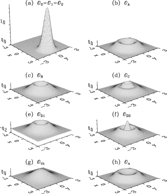
FIG. 1.: The reconstructed Wigner functions of the coherent state $|\alpha\rangle$ with $\bar{n}=2$. We consider the observation levels as indicated in the figure. It is clearly seen that the Wigner function of a coherent state can be easily reconstructed on the most simple phase-sensitive observation level ${\cal O}_{1}$. We note that on some observation levels the reconstructed Wigner function of the coherent state may take negative values.

from which we see that the Wigner function (231) is positive. We plot $W^{\rm(A)}_{|\alpha\rangle}(\xi)$ in Fig. 1b. We can understand the shape of $W^{\rm(A)}_{|\alpha\rangle}(\xi)$ if we imagine phase-averaging of the Wigner function $W_{|\alpha\rangle}(\xi)$ [see Fig. 1a]. On the other hand we can represent $W^{\rm(A)}_{|\alpha\rangle}(\xi)$ as a sum of weighted Wigner functions of Fock states [see Eq.(230)]. For the considered coherent state $|\alpha\rangle$ with the mean photon number $\bar{n}=2$ we have $P_{1}=P_{2}=2P_{0}=2\exp(-2)$, so the Wigner functions of Fock states $|1\rangle$ and $|2\rangle$ dominantly contribute to $W^{\rm(A)}_{|\alpha\rangle}(\xi)$. On the other hand contribution of the Wigner function of the vacuum state is suppressed and therefore $W^{\rm(A)}_{|\alpha\rangle}(\xi)$ has a local minimum around the origin of the phase space while its maximum is at the same distance from the origin of the phase space as for the Wigner function on the complete observation level [see Fig. 1a]. We note that the Wigner function $W^{\rm(A)}_{|\alpha\rangle}(\xi)$ describing the phase-diffused coherent state has been experimentally reconstructed recently by Munroe et al. [11].

2 Observation level ${\cal O}_{\rm B}$

Let us assume that from a measurement the mean photon number $\bar{n}$ and probabilities $P_{2n}$ are know (see Section IV C 2). If the values of $P_{2n}$ are given by Poissonian distribution (228), i.e., $P_{2n}=\exp(-\bar{n})\bar{n}^{2n}/(2n)!$, then using definitions (178) and (179) we can find the parameters $P_{odd}$ and $\bar{n}_{odd}$ to be

$$P_{odd}={\rm e}^{-\bar{n}}\sinh\bar{n};\qquad\bar{n}_{odd}=\bar{n}(1-P_{odd}),$$ (233)

The reconstructed probabilities $P_{2n+1}$ are given by Eq.(182) and in the limit of large $\bar{n}$ (when $P_{odd}\to 1/2$ and $\bar{n}_{odd}\to\bar{n}/2$) they read

$$P_{2n+1}\rightarrow\frac{(\bar{n}-1)^{n}}{(\bar{n}+1)^{n+1}}.$$ (234)

With the help of the relation (175) and explicit expressions for $P_{2n}$ and $P_{2n+1}$ we can evaluate expression for the Wigner function of the coherent state on the observation level ${\cal O}_{\rm B}$. We plot $W^{\rm(B)}_{|\alpha\rangle}(\xi)$ of the coherent state with the mean photon number equal to two ($\bar{n}=2$) in Fig. 1c. In this case $P_{2}$ is dominant from which it follows that the Fock state $|2\rangle$ gives a significant contribution into $W^{\rm(B)}_{|\alpha\rangle}(\xi)$ [compare with Fig. 1b].

3 Observation level ${\cal O}_{\rm C}$

The Wigner function $W^{(C)}_{|\alpha\rangle}(\xi)$ of the coherent state on the observation level ${\cal O}_{\rm C}$ can be reconstructed in exactly same way as on the level ${\cal O}_{\rm B}$. In Fig. 1d we present a result of this reconstruction. On the observation level ${\cal O}_{\rm C}$ the contribution of the vacuum state is more significant than in the case ${\cal O}_{\rm B}$ which is due to the thermal-like photon number distribution $P_{2n}$ on the even-number subspace of the Fock space [see Eq.(184)].

4 Observation level ${\cal O}_{\rm D1}$

We can easily reconstruct the Wigner function of the coherent state at the observation level ${\cal O}_{\rm D1}$. Using general expressions from Section IV C 4 we find the following expression for the Wigner function $W^{\rm(D1)}_{|\alpha\rangle}(\xi)$ [we remind us that for coherent state the parameter $P_{0}$ is given by the relation $P_{0}=\exp(-\bar{n})\,$]:

$$W^{\rm(D1)}_{|\alpha\rangle}(\xi)=\left(P_{0}-\frac{1-P_{0}}{\tilde{n}}\right)W_{|0\rangle}(\xi)+(1-P_{0})\frac{\tilde{n}+1}{\tilde{n}}W_{\rm th}(\xi),$$ (235)

where $W_{|0\rangle}(\xi)$ is the Wigner function of the vacuum state given by Eq.(89) and $W_{\rm th}(\xi)$ is the Wigner function of a thermal state (136) with an effective number of photons equal to $\tilde{n}$, where

$$\tilde{n}=\frac{\bar{n}}{1-P_{0}}-1.$$ (236)

In particular, from Eqs.(235) and (236) it follows that

$$\lim_{\bar{n}\rightarrow 0}W^{\rm(D1)}_{|\alpha\rangle}(\xi)=W_{|0\rangle}(\xi),$$ (237)

and simultaneously $S_{\rm D1}=0$, which means that the vacuum state can be completely reconstructed on the present observation level. Another result which can be derived from Eq.(235) is that if $P_{0}(2\bar{n}+1)<1$, then the reconstructed Wigner function $W^{\rm(D1)}_{|\alpha\rangle}(\xi)$ of the coherent state $|\alpha\rangle$ can be negative due to the fact that the contribution of the Fock state $|1\rangle$ is more dominant than the contribution of the vacuum state and then the negativity of the Wigner function $W_{|1\rangle}(\xi)$ results into negative values of $W^{\rm(D1)}_{|\alpha\rangle}(\xi)$. This means that even though the Wigner function of the state itself (i.e., the Wigner function at the complete observation level) is positive, the reconstructed Wigner function can be negative. This is a clear indication that the observation level has to be chosen very carefully and that reconstructed Wigner functions can indicate nonclassical behavior even in those cases when the measured state itself does not exhibit nonclassical effects. In Fig. 1e we plot the Wigner function $W^{\rm(D1)}_{|\alpha\rangle}(\xi)$ of the coherent state which illustrates this effect.

5 Observation level ${\cal O}_{\rm D2}$

If the mean photon number $\bar{n}$ is an integer, then one may consider the observation level ${\cal O}_{\rm D2}$. The Wigner function of the coherent state at this observation level for which $P_{\bar{n}}=\exp(-\bar{n})\bar{n}^{\bar{n}}/(\bar{n}!)$ reads

$$W^{\rm(D2)}_{|\alpha\rangle}(\xi)=\left(1-\frac{1+\bar{n}}{Z_{\rm D2}}\right)W_{|\bar{n}\rangle}(\xi)+\frac{\bar{n}+1}{Z_{\rm D2}}W_{\rm th}(\xi),$$ (238)

where $W_{|\bar{n}\rangle}(\xi)$ is the Wigner function of the Fock state $|\bar{n}\rangle$ and $W_{\rm th}(\xi)$ is the Wigner function of the thermal state with the mean photon number equal to $\bar{n}$. The partition function $Z_{\rm D2}$ is given by the relation (204). The Wigner function (238) is plotted in Fig. 1f. From this figure we see that the vacuum state $|0\rangle$ (due to the thermal-like character of the reconstructed photon number distribution) and the Fock state $|2\rangle$ (as a consequence of the measurement) dominantly contribute to $W^{\rm(D1)}_{|\alpha\rangle}(\xi)$.

B Squeezed vacuum

The Wigner function of the squeezed vacuum state (108) on the complete observation level ${\cal O}_{0}$ is given by Eq.(112) and is plotted (in the complex $\xi$ phase space) in Fig. 2a. This is a Gaussian function, which carries phase information associated with the phase of squeezing. On the thermal observation level ${\cal O}_{\rm th}$ which is characterized only by the mean photon number $\bar{n}$ the reconstructed Wigner function of the squeezed vacuum state is a rotationally symmetrical Gaussian function centered at the origin of the phase space [see Eq.(136) and Fig. 1g]. On the observation level ${\cal O}_{\rm 1}$ the reconstructed Wigner function is the same as on the thermal observation level because the mean amplitudes $\langle\hat{a}\rangle$ and $\langle\hat{a}^{\dagger}\rangle$ are equal to zero. On the other hand, the Wigner function of the squeezed vacuum can be completely reconstructed on the observation level ${\cal O}_{\rm 2}$. To see this we evaluate the entropy $S_{2}$ for the squeezed vacuum state [see Eq.(159)]. The parameters $M$ and $N$ can be expressed in terms of the squeezing parameter $\eta$ (we assume $\eta$ to be real) as

$$N=\frac{\eta^{2}}{1-\eta^{2}};\qquad M=\frac{\eta}{1-\eta^{2}},$$ (239)

so that $N(N+1)=M^{2}$. Consequently the parameter $\chi$ given by Eq.(156) is equal to zero from which it follows that $S_{2}$ for the squeezed vacuum is equal to zero.

1 Observation level ${\cal O}_{\rm A}$

The squeezed vacuum state (108) is characterized by the oscillatory photon number distribution $P_{n}$:

$$P_{2n}=(1-\eta^{2})^{1/2}\frac{(2n)!}{[2^{n}n!]^{2}}\eta^{2n};\qquad P_{2n+1}=0.$$ (240)

Using Eq.(175) we can express the Wigner function $W_{|\eta\rangle}^{(A)}(\xi)$ of the squeezed vacuum on the observation level ${\cal O}_{\rm A}$ as

$$W_{|\eta\rangle}^{(A)}(\xi)=2(1-\eta^{2})^{1/2}{\rm e}^{-2|\xi|^{2}}\sum_{n=0}^{\infty}\frac{(2n)!\eta^{2n}}{2^{2n}(n!)^{2}}{\cal L}_{2n}(4|\xi|^{2}).$$ (241)

Taking into account that the Wigner function on the observation level ${\cal O}_{\rm A}$ can be obtained as the phase-averaged Wigner function on the complete observation level, we can rewrite (241) as

$$W_{|\eta\rangle}^{(A)}(\xi)=\frac{1}{2\pi}\int_{-\pi}^{\pi}W_{|\eta\rangle}(\xi)d\phi;\qquad\xi=|\xi|{\rm e}^{i\phi}.$$ (242)

If we insert the explicit expression for $W_{|\eta\rangle}(\xi)$ [see Eq.(112)] into Eq.(242) we obtain

$$W_{|\eta\rangle}^{(A)}(\xi)=2\exp\left[-\left(\frac{|\xi|^{2}}{2\sigma_{q}^{2}}+\frac{|\xi|^{2}}{2\sigma_{p}^{2}}\right)\right]I_{0}\left(\frac{|\xi|^{2}}{2\sigma_{q}^{2}}-\frac{|\xi|^{2}}{2\sigma_{p}^{2}}\right),$$ (243)

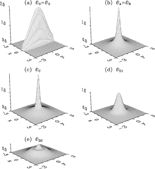
FIG. 2.: The reconstructed Wigner functions of the squeezed vacuum state $|\eta\rangle$ with $\bar{n}=2$. We consider the observation levels as indicated in the figure. This Wigner function can be completely reconstructed on the observation level ${\cal O}_{2}$.

where $I_{0}(x)$ is the modified Bessel function. We plot this Wigner function in Fig. 2b. We see that $W_{|\eta\rangle}^{(A)}(\xi)$ is not negative and that it is much narrower in the vicinity of the origin of the phase space than the Wigner function of the vacuum state (compare with Fig. 1a). Nevertheless the total width of Wigner function $W^{\rm(A)}_{|\eta\rangle}(\xi)$ is much larger than the width of the Wigner function of the vacuum state.

2 Observation level ${\cal O}_{\rm B}$

Due to the fact that for the squeezed vacuum state we have $\sum_{n}P_{2n}=1$, the Wigner function of the squeezed vacuum state on the observation level ${\cal O}_{\rm B}$ is equal to the Wigner function on the observation level ${\cal O}_{\rm A}$, i.e., $W_{|\eta\rangle}^{(B)}(\xi)=W_{|\eta\rangle}^{(A)}(\xi)$.

3 Observation level ${\cal O}_{\rm C}$

For the squeezed vacuum state all meanvalues $P_{2n+1}$ are equal to zero and therefore $\sum_{n}P_{2n+1}=0$. From this fact and from the knowledge of the mean photon number $\bar{n}$ we can reconstruct the Wigner function $W_{|\eta\rangle}^{(C)}(\xi)$ in the form [see Section IV B 3]

$$W_{|\eta\rangle}^{(C)}(\xi)=\frac{4{\rm e}^{-2|\xi|^{2}}}{\bar{n}+2}\sum_{k=0}^{\infty}\left(\frac{\bar{n}}{\bar{n}+2}\right)^{k}{\cal L}_{2k}(4|\xi|^{2}),$$ (244)

where $\bar{n}$ is the mean photon number in the squeezed vacuum state. We plot the Wigner function $W_{|\eta\rangle}^{(C)}(\xi)$ in Fig. 2c. This Wigner function is very similar to the Wigner function on the observation level ${\cal O}_{\rm A}$ [see Fig. 2b] which reflects the fact that the photon number distribution of the squeezed vacuum state has a thermal-like character on the even-number subspace of the Fock space.

4 Observation level ${\cal O}_{\rm D1}$

With the help of the general formalism presented in Section IV we can express the Wigner function $W_{|\eta\rangle}^{(D1)}(\xi)$ of the squeezed vacuum state on the observation level ${\cal O}_{\rm D1}$ in the form [see Eq.(235)] with

$$P_{0}=(1-\eta^{2})^{1/2}=(\bar{n}+1)^{-1/2};\qquad\mbox{and}~{}~{}~{}\tilde{n}=\frac{\bar{n}}{1-(1+\bar{n})^{-1/2}}-1.$$ (245)

We plot the Wigner function $W_{|\eta\rangle}^{(D1)}(\xi)$ in Fig. 2d from which the dominant contribution of the vacuum state is transparent which is due to the fact that the squeezed vacuum state has a thermal-like photon number distribution.

5 Observation level ${\cal O}_{\rm D2}$

If we consider $\bar{n}$ to be an even integer, then the Wigner function $W_{|\eta\rangle}^{(D2)}(\xi)$ of the squeezed vacuum state on ${\cal O}_{\rm D2}$ is given by Eq.(238). The partition function $Z_{\rm D2}$ is given by Eq.(204) where

$$P_{\bar{n}}=\frac{\bar{n}!}{2^{\bar{n}}\left[(\bar{n}/2)!\right]^{2}}\frac{\bar{n}^{\bar{n}/2}}{(1+\bar{n})^{(1+\bar{n})/2}}.$$ (246)

We plot this Wigner function in Fig. 2e. It has a thermal-like character [compare with Fig. 1g] but contribution of the Fock state $|\bar{n}=2\rangle$ is more dominant compared with the proper thermal distribution. If $\bar{n}$ is an odd integer, then $P_{\bar{n}}=0$ and the corresponding Wigner function can be again reconstructed with the help of Eqs.(238) and (204).

C Even coherent state

We plot the Wigner function of the even coherent state on the complete observation level in Fig. 3a. Two contributions of coherent component state $|\alpha\rangle$ and $|-\alpha\rangle$ as well as the interference peak around the origin of the phase space are transparent in this figure. As in the case of the squeezed vacuum state, the mean amplitude $\langle\hat{a}\rangle$ of the even coherent state is equal to zero and therefore the Wigner function $W_{|\alpha_{e}\rangle}^{(1)}(\xi)$ of the even coherent state on the observation level ${\cal O}_{1}$ is equal to the thermal Wigner function given by Eq.(136).

1 Observation level ${\cal O}_{\rm 2}$

Using general expressions from Section IV A 2 we can express the Wigner function $W_{|\alpha_{e}\rangle}^{(2)}(\xi)$ of the even coherent state on the observation level ${\cal O}_{2}$ as

$$W_{|\alpha_{e}\rangle}^{(2)}(\xi)=\frac{1}{\left[(N+1/2)^{2}-M^{2}\right]^{1/2}}\exp\left[-\frac{\xi_{x}^{2}}{[(N+1/2)+M]}-\frac{\xi_{y}^{2}}{[(N+1/2)-M]}\right],$$ (247)

where $\xi=\xi_{x}+i\xi_{y}$, and the parameters $N$ and $M$ read

$$N=\alpha^{2}\tanh\alpha^{2};\qquad M=\alpha^{2}.$$ (248)

We plot the Wigner function $W_{|\alpha_{e}\rangle}^{(2)}(\xi)$ in Fig. 3b. This Wigner function is slightly “squeezed” in the $\xi_{y}$-direction and stretched in the $\xi_{x}$-direction. Nevertheless, the reconstructed Wigner function is different from the Wigner function of the squeezed vacuum state [compare with Fig. 2a].

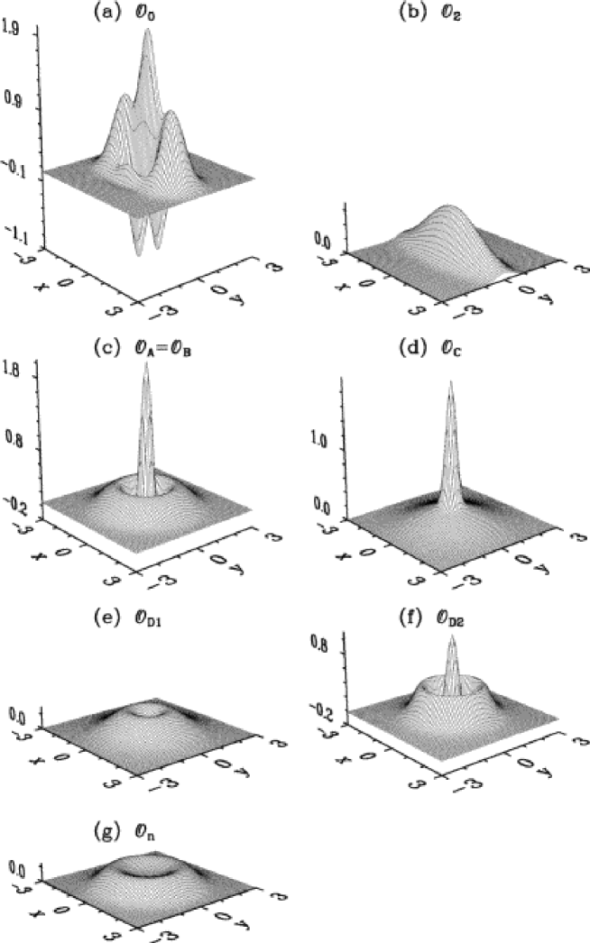
FIG. 3.: The reconstructed Wigner functions of the even coherent state $|\alpha_{e}\rangle$ with $\bar{n}=2$. We consider the observation levels as indicated in the figure. This non-Gaussian Wigner function can be completely reconstructed only on the complete observation level when all moments of systems operators are measured.

2 Observation level ${\cal O}_{\rm A}$

The photon number distribution of the even coherent state is given by the relation (we assume $\alpha$ to be real):

$$P_{2n}=\frac{1}{\cosh\alpha^{2}}\frac{\alpha^{4n}}{(2n)!};\qquad P_{2n+1}=0,$$ (249)

so the corresponding Wigner function can be expressed as Eq.(175). We can also express $W_{|\alpha_{e}\rangle}^{(A)}(\xi)$ as the phase averaged Wigner function of the even coherent state $W_{|\alpha_{e}\rangle}(\xi)$ given by Eq.(116). After some algebra we find that $W_{|\alpha_{e}\rangle}^{(A)}(\xi)$ can be written in a closed form

$$W_{|\alpha_{e}\rangle}^{(A)}(\xi)=\frac{{\rm e}^{-2|\xi|^{2}}}{\cosh\alpha^{2}}\left[{\rm e}^{-\alpha^{2}}J_{0}(4i\alpha|\xi|)+{\rm e}^{\alpha^{2}}J_{0}(4\alpha|\xi|)\right].$$ (250)

We plot the Wigner function $W_{|\alpha_{e}\rangle}^{(A)}(\xi)$ in Fig. 3c. From this figure the dominant contribution of the Fock state $|2\rangle$ is transparent (in the present case we have $P_{0}\simeq 2\exp(-2)$, $P_{2}=2P_{0}$, and $P_{4}=2P_{0}/3$, while all other probabilities $P_{n}$ are much smaller) which results in negative Wigner function.

3 Observation level ${\cal O}_{\rm B}$

Due to the fact that the even coherent state is expressed as a superposition of only even Fock states, i.e., $\sum_{n}P_{2n}=1$, the Wigner functions on the observation levels ${\cal O}_{\rm A}$ and ${\cal O}_{\rm B}$ are equal, i.e., $W_{|\alpha_{e}\rangle}^{(B)}(\xi)=W_{|\alpha_{e}\rangle}^{(A)}(\xi)$.

4 Observation level ${\cal O}_{\rm C}$

As a consequence of the fact that for the even coherent state all meanvalues $P_{2n+1}$ are equal to zero the information available for the reconstruction of the Wigner function $W_{|\alpha_{e}\rangle}^{(C)}(\xi)$ is the same as in the case of the reconstruction of the Wigner function of the squeezed vacuum state on the observation level ${\cal O}_{\rm C}$. Therefore, the Wigner function $W_{|\alpha_{e}\rangle}^{(C)}(\xi)$ has exactly the same form as for the squeezed vacuum state with the same mean photon number $\bar{n}$ [see Fig. 3d and Fig. 2c].

5 Observation level ${\cal O}_{\rm D1}$

The Wigner function $W_{|\alpha_{e}\rangle}^{(D1)}(\xi)$ of the even coherent state on the observation level ${\cal O}_{\rm D1}$ is given by Eq.(235) with

$$P_{0}=\frac{1}{\cosh\alpha^{2}};\qquad\tilde{n}=\frac{\alpha^{2}\sinh\alpha^{2}}{\cosh\alpha^{2}-1}-1.$$ (251)

We plot the Wigner function $W_{|\alpha_{e}\rangle}^{(D1)}(\xi)$ in Fig. 3e. This Wigner function has a thermal-like character except the fact that the contribution of the vacuum state is slightly suppressed.

6 Observation level ${\cal O}_{\rm D2}$

Analogously we can find the Wigner function $W_{|\alpha_{e}\rangle}^{(D2)}(\xi)$. If we consider $\bar{n}$ to be an even integer, then the Wigner function $W_{|\eta\rangle}^{(D2)}(\xi)$ of the even coherent state on ${\cal O}_{\rm D2}$ is given by Eq.(238) and Eq.(204) where

$$P_{\bar{n}}=\frac{1}{\cosh\alpha^{2}}\frac{\alpha^{2\bar{n}}}{\bar{n}!},$$ (252)

and if $\bar{n}$ is an odd integer then $P_{\bar{n}}=0$. We plot $W_{|\alpha_{e}\rangle}^{(D2)}(\xi)$ in Fig. 3f. From our previous discussion it is clear that in the present case the vacuum state and the Fock state $|2\rangle$ dominantly contribute to $W_{|\alpha_{e}\rangle}^{(D2)}(\xi)$ (similarly as on the observation level ${\cal O}_{\rm A}$ - see Fig. 3c).

D Odd coherent state

We present the Wigner function of the odd coherent state with the mean photon number equal to two in Fig. 4a. The mean amplitude $\langle\hat{a}\rangle$ of the odd coherent state is equal to zero and therefore the Wigner function $W_{|\alpha_{o}\rangle}^{(1)}(\xi)$ of this state on the observation level ${\cal O}_{1}$ is equal to the thermal Wigner function given by Eq.(136) [see Fig. 1g].

1 Observation level ${\cal O}_{\rm 2}$

Using general expressions from Section IV B 2 we find that the Wigner function $W_{|\alpha_{o}\rangle}^{(2)}(\xi)$ of the odd coherent state on the observation level ${\cal O}_{2}$ is the same as for the even coherent state [see Eq.(247)] but the parameters $N$ and $M$ in the present case read

$$N=\alpha^{2}\coth\alpha^{2};\qquad M=\alpha^{2}.$$ (253)

We plot the Wigner function $W_{|\alpha_{o}\rangle}^{(2)}(\xi)$ in Fig. 4b. This is a “squeezed”-Gaussian function similar to the Wigner function of the even coherent state on the same observation level [see Fig. 3b and discussion in the previous section].

2 Observation level ${\cal O}_{\rm A}$

The photon number distribution of the odd coherent state is given by the relation (we assume $\alpha$ to be real):

$$P_{2n}=0;\qquad P_{2n+1}=\frac{1}{\sinh\alpha^{2}}\frac{(\alpha^{2})^{2n+1}}{(2n+1)!}.$$ (254)

Consequently, the Wigner function $W_{|\alpha_{o}\rangle}^{(A)}(\xi)$ can be expressed as (175). Alternatively, if we use the fact that $W_{|\alpha_{o}\rangle}^{(A)}(\xi)$ is equal to the phase averaged Wigner function of the odd coherent state $W_{|\alpha_{o}\rangle}(\xi)$ given by Eq.(117), then we can write

$$W_{|\alpha_{o}\rangle}^{(A)}(\xi)=\frac{{\rm e}^{-2|\xi|^{2}}}{\sinh\alpha^{2}}\left[{\rm e}^{-\alpha^{2}}J_{0}(4i\alpha|\xi|)-{\rm e}^{\alpha^{2}}J_{0}(4\alpha|\xi|)\right].$$ (255)

This function is always negative in the origin of the phase space. We plot the Wigner function $W_{|\alpha_{o}\rangle}^{(A)}(\xi)$ in Fig. 4c. In the present case $P_{0}=P_{2}=0$ and the $P_{1}$ is the largest probability therefore the contribution of the Fock state $|1\rangle$ in $W_{|\alpha_{o}\rangle}^{(A)}(\xi)$ is the most dominant which is clearly seen from Fig. 4c. We also note that, in general, any superposition of odd Fock states has a negative Wigner function on the observation level ${\cal O}_{\rm A}$.

3 Observation level ${\cal O}_{\rm B}$

For the odd coherent state all meanvalues $P_{2n}$ are equal to zero. Taking into account this information and the information about the mean photon number we reconstruct the Wigner function $W_{|\alpha_{o}\rangle}^{(B)}(\xi)$ in the form (for details see Section  IV C 2)

$$W_{|\alpha_{o}\rangle}^{(B)}(\xi)=-\frac{4{\rm e}^{-2|\xi|^{2}}}{\bar{n}+1}\sum_{k=0}^{\infty}\left(\frac{\bar{n}-1}{\bar{n}+1}\right)^{k}{\cal L}_{2k+1}(4|\xi|^{2}),$$ (256)

where $\bar{n}=\alpha^{2}\coth\alpha^{2}$. We plot this Wigner function in Fig. 4d. In the present case the dominant contribution of the Fock state $|1\rangle$ is seen ($P_{0}=P_{2}=0$ and due to the thermal-like photon number distribution on the odd-number subspace of the Fock state $P_{3}$ is much smaller than $P_{1}$). We can conclude, that any superposition of odd Fock states on the observation level ${\cal O}_{\rm B}$ has the Wigner function given by Eq.(256), i.e., superpositions of odd Fock states are indistinguishable on ${\cal O}_{\rm B}$.

4 Observation level ${\cal O}_{\rm C}$

Due to the fact that the odd coherent state is expressed as a superposition of only odd Fock states, i.e., $\sum_{n}P_{2n+1}=1$, the Wigner functions on the observation levels ${\cal O}_{\rm C}$ and ${\cal O}_{\rm A}$ are equal, i.e., $W_{|\alpha_{o}\rangle}^{(C)}(\xi)=W_{|\alpha_{o}\rangle}^{(A)}(\xi)$.

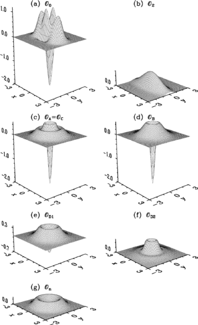
FIG. 4.: The reconstructed Wigner functions of the odd coherent state $|\alpha_{o}\rangle$ with $\bar{n}=2$. We consider the observation levels as indicated in the figure.

5 Observation level ${\cal O}_{\rm D1}$

The Wigner function $W_{|\alpha_{o}\rangle}^{(D1)}(\xi)$ of the odd coherent state on the observation level ${\cal O}_{\rm D1}$ is given by the following relation [we remind us that for the odd coherent state we have $P_{0}=0$]

$$W_{|\alpha_{o}\rangle}^{(D1)}(\xi)=-\frac{1}{\bar{n}-1}W_{|0\rangle}(\xi)+\frac{\bar{n}}{\bar{n}-1}W_{\rm th}(\xi),$$ (257)

where $\bar{n}$ is the mean photon number in the odd coherent state; $W_{|0\rangle}(\xi)$ is the Wigner function of the vacuum state and $W_{\rm th}(\xi)$ is the thermal Wigner function for the state with $\bar{n}-1$ photons. We note that from Eq.(257) it follows that

$$\lim_{\bar{n}\rightarrow 1}W_{|\alpha_{o}\rangle}^{(D1)}(\xi)=W_{|1\rangle}(\xi),$$ (258)

We plot the Wigner function $W_{|\alpha_{o}\rangle}^{(D1)}(\xi)$ in Fig. 4e. Compared with Fig. 4d we see that the contribution of the Fock state $|1\rangle$ on the observation level ${\cal O}_{\rm D1}$ is smaller than on ${\cal O}_{\rm B}$. This is due to the fact that on the present observation level $P_{2}$ is not equal to zero.

6 Observation level ${\cal O}_{\rm D2}$

Reconstruction of the Wigner function $W_{|\alpha_{o}\rangle}^{(D2)}(\xi)$ is straightforward. For the odd coherent state it is valid that if $\bar{n}$ is an odd integer, then

$$P_{\bar{n}}=\frac{1}{\sinh\alpha^{2}}\frac{\alpha^{2\bar{n}}}{\bar{n}!},$$ (259)

and the Wigner function is given by Eq.(238). On the other hand if $\bar{n}$ is an even integer, then $P_{\bar{n}}=0$ and we again use Eq.(238) for the reconstruction of the Wigner function $W_{|\eta\rangle}^{(D2)}(\xi)$. We plot this Wigner function in Fig. 4f. Even though on this observation level $P_{2}=0$ the contribution from the vacuum state is significant and therefore $W_{|\alpha_{o}\rangle}^{(D2)}(\xi)$ is not negative in the present case.

E Fock state

Mean values of the operators $\hat{a}^{k}$ in the Fock state are equal to zero, therefore the Wigner functions $W_{|n\rangle}^{(1)}(\xi)$ and $W_{|n\rangle}^{(2)}(\xi)$ of the Fock state $|n\rangle$ on the observation levels ${\cal O}_{1}$ and ${\cal O}_{2}$, respectively, are equal to the thermal Wigner function given by Eq.(136) [see Fig. 5b]. On the other hand the Shannon entropy of the Fock state is equal to zero, therefore this state can be completely reconstructed on the observation level ${\cal O}_{\rm A}$ [see Fig. 5a for the Wigner function of the Fock state $|2\rangle$].

1 Observation level ${\cal O}_{\rm B}$

If the Fock state has an even number of photons then it can also be completely reconstructed on the observation level ${\cal O}_{\rm B}$. But if the number of photons of the Fock state is odd then the Wigner function of this Fock state on ${\cal O}_{\rm B}$ is given by the relation (256) with $\bar{n}=n$.

2 Observation level ${\cal O}_{\rm C}$

If the number of photons on the Fock state is odd than the corresponding Wigner function can be completely reconstructed on the observation level ${\cal O}_{\rm C}$. If the number of photons is even, then the Wigner function $W_{|n\rangle}^{(C)}(\xi)$ is given by Eq.(244) with $\bar{n}=n$. We plot $W_{|n\rangle}^{(C)}(\xi)$ in Fig. 5c. This Wigner function is the same as for the squeezed vacuum state $W_{|\eta\rangle}^{(C)}(\xi)$ and the even coherent state $W_{|\alpha_{e}\rangle}^{(C)}(\xi)$ with the same mean photon number [see Figs. 2c and 3d]. More generally, all superpositions of even Fock states with the same mean photon number are indistinguishable on ${\cal O}_{\rm C}$.

3 Observation level ${\cal O}_{\rm D1}$

If the Fock state under consideration is the vacuum state then it can be completely reconstructed on the observation level ${\cal O}_{\rm D1}$. If the number of photons is larger than zero, then $P_{0}=0$ and the corresponding Wigner function is given by Eq.(257) with $\bar{n}=n$. We plot $W_{|n=2\rangle}^{(D1)}(\xi)$ in Fig. 5d.

4 Observation level ${\cal O}_{\rm D2}$

On this observation level the Wigner function of the Fock state $|n\rangle$ can be always completely reconstructed, because this observation level is defined in such way that $P_{n}=1$.

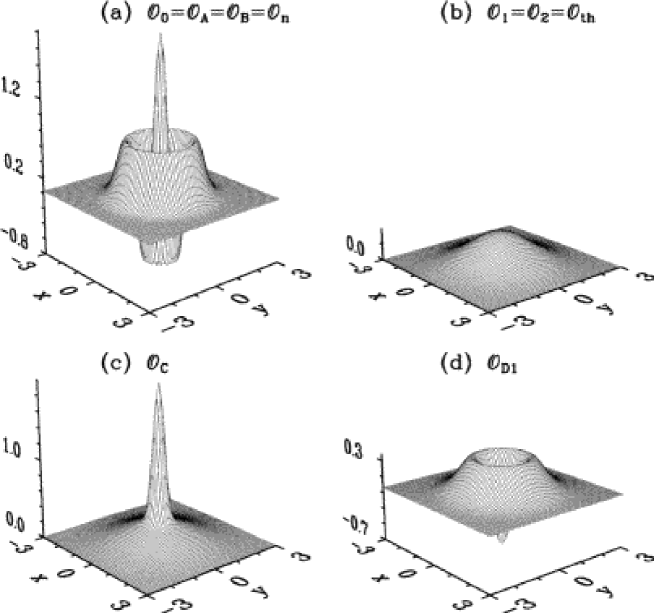
FIG. 5.: The reconstructed Wigner functions of the Fock state $|n=2\rangle$. We consider the observation levels as indicated in the figure. Even though the Fock state is represented by the non-Gaussian Wigner function it can be completely reconstructed on the observation level ${\cal O}{\rm n}$.

F Observation level ${\cal O}_{\rm n}\equiv\{\hat{n},\hat{n}^{2}\}$

We will finish this section with a brief discussion about the phase-insensitive observation level ${\cal O}_{\rm n}$ which is related to a measurement of the observables $\hat{n}$ and $\hat{n}^{2}$.

The generalized canonical density operator $\hat{\sigma}$ on the observation level ${\cal O}_{\rm n}$ reads:

$$\hat{\sigma}_{\rm n}=\frac{1}{Z_{\rm n}}\exp\left[-\lambda_{1}\hat{n}-\lambda_{2}\hat{n}^{2}\right]=\frac{1}{Z_{\rm n}}\sum_{n=0}^{\infty}\exp\left[-\lambda_{1}n-\lambda_{2}n^{2}\right]|n\rangle\langle n|.$$ (260)

The Lagrange multipliers are determined by the relations

$$\langle\hat{n}\rangle=-\frac{\partial\ln Z_{\rm n}}{\partial\lambda_{1}}=\sum_{m=0}^{\infty}mP_{m};$$ (261)

$$\langle\hat{n}^{2}\rangle=-\frac{\partial\ln Z_{\rm n}}{\partial\lambda_{2}}=\sum_{m=0}^{\infty}m^{2}P_{m},$$ (262)

where

$$P_{m}=\frac{1}{Z_{\rm n}}\exp\left[-\lambda_{1}m-\lambda_{2}m^{2}\right];$$ (263)

and

$$Z_{\rm n}=\sum_{m=0}^{\infty}\exp\left[-\lambda_{1}m-\lambda_{2}m^{2}\right].$$ (264)

From Eqs.(261) and (262) it follows that if $\langle\hat{n}\rangle=N$ is an integer, then in the limit $\sigma_{n}\rightarrow 0_{+}$ (where $\sigma_{n}^{2}\equiv\langle\hat{n}^{2}\rangle-\langle\hat{n}\rangle^{2}$) $\lambda_{1}=-2N\lambda_{2}$ and $\lambda_{2}$ tends to infinity. Simultaneously

$$P_{m}\rightarrow\delta_{m,N},$$ (265)

which means that in this case $\hat{\sigma}_{\rm n}\rightarrow|N\rangle\langle N|$. In other words, on the observation level ${\cal O}_{\rm n}$ the Fock state $|N\rangle$ can be completely reconstructed (see Fig.5a) and in this case the corresponding entropy $S_{\rm n}=-k_{B}\sum_{m}P_{m}\ln P_{m}$ is equal to zero.

The Wigner function of this state is negative, which in particular reflects the fact that the reconstructed distribution is narrower than the Poissonian (coherent-state) photon number distribution, i.e., the state under consideration exhibits sub-Poissonian photon number distribution. To quantify the degree of the sub-Poissonian photon statistics one can utilize the Mandel $Q$ parameter defined as:

$$Q=\frac{\langle\hat{n}^{2}\rangle-\langle\hat{n}\rangle^{2}-\langle\hat{n}\rangle}{\langle\hat{n}\rangle},$$ (266)

which for Fock states is equal to -1 while for coherent states is equal to 0. The state is said to have sub-Poissonian photon statistics providing $Q<0$. One can easily reconstruct sub-Poissonian states on the observation level ${\cal O}_{\rm n}$. In addition states with the Poissonian photon statics $Q=0$ can be partially reconstructed on this observation level as well. For instance in Fig.1h we represent a result of numerical reconstruction of the Wigner function $W^{(\rm n)}_{|\alpha\rangle}(\xi)$ of the coherent state with a Poissonian photon number distribution on the observation level ${\cal O}_{\rm n}$. In this case the reconstructed photon number distribution $P_{n}$ [see Eq.(263)] does not have a Poissonian character, and therefore the reconstructed Wigner functions of the coherent state on the observation levels ${\cal O}_{\rm A}$ and ${\cal O}_{\rm n}$ are different (compare Figs.1b and 1h, respectively) even though the reconstructed states have the same mean photon number $\langle\hat{n}\rangle$ and the same variance $\sigma_{n}^{2}$ in the photon number distribution.

On the observation level ${\cal O}_{\rm n}$ we can reconstruct also the odd coherent state given by Eq.(115) which is a sub-Poissonian state with the $Q$ parameter given by the relation (we assume $\alpha$ to be real):

$$Q=-\frac{4\alpha^{2}{\rm e}^{-2\alpha^{2}}}{1-{\rm e}^{-4\alpha^{2}}}=-\frac{\bar{n}}{(\cosh\alpha^{2})^{2}}<0,$$ (267)

where the mean photon number $\bar{n}$ in the odd coherent state is given by the relation $\bar{n}=\alpha^{2}\coth\alpha^{2}$. We have plotted the result of the numerical reconstruction of the Wigner function of the odd coherent state with $\bar{n}=2$ on the given observation level in Fig.4g. Due to the fact, that for the given mean photon number the odd coherent state does not exhibit a significant degree of sub-Poissonian photon statistics, the corresponding Wigner function $W^{(\rm n)}_{|\alpha_{o}\rangle}(\xi)$ is not negative (compare with Fig.4c).

The even coherent state (114) is characterized by the super-Poissonian photon statistics with the Mandel $Q$ parameter given by the relation

$$Q=\frac{4\alpha^{2}{\rm e}^{-2\alpha^{2}}}{1-{\rm e}^{-4\alpha^{2}}}=\frac{\bar{n}}{(\sinh\alpha^{2})^{2}}>0,$$ (268)

with the mean photon number given by the relation $\bar{n}=\alpha^{2}\tanh\alpha^{2}$. From Eq.(268) it follows that for large enough values of $\alpha$ (i.e., for large enough values of $\bar{n}$) the Mandel $Q$ parameter is smaller than $\bar{n}$ (it tends to zero). In this case the Wigner function of the even coherent state on the observation level ${\cal O}_{\rm n}$ can be easily reconstructed (see Fig.3g). We can also reconstruct on this observation level a thermal mixture for which the Mandel $Q$ parameter is equal to $\bar{n}$ (i.e., $\langle\hat{n}^{2}\rangle=2\bar{n}^{2}+\bar{n}$) In this case the Lagrange multiplier $\lambda_{2}$ in expression (260) is equal to zero and consequently the results of the reconstruction on the observation levels ${\cal O}_{\rm n}$ and ${\cal O}_{\rm th}$ (thermal observation level) are equal.

It is important to stress that all those states for which the Mandel $Q$ parameter is less than $\bar{n}$ (in analogy with sub-Poissonian states we can call these states as the sub-thermal states) can be reconstructed on ${\cal O}_{\rm n}$. For all these states the Lagrange multiplier $\lambda_{2}$ is greater than zero and consequently the generalized partition function (264) does exist. Nevertheless there are states for which $Q>\bar{n}$ (we will call these states as super-thermal states). For these state the Lagrange multiplier $\lambda_{2}$ is smaller than zero and $Z_{\rm n}$ given by Eq.(264) is diverging. Consequently, these states cannot be reconstructed on the observation level ${\cal O}_{\rm n}$. In particular, the Mandel $Q$ parameter for the squeezed vacuum state (108) reads $Q=2\bar{n}+1$ (for $\bar{n}>0$) and therefore we are not able to reconstruct the Wigner function of the squeezed vacuum state on ${\cal O}_{\rm n}$. Analogously, the even coherent state for small values of $\alpha$ such that $\sinh\alpha^{2}<1$ has a super-thermal photon number distribution and it cannot be reconstructed on this observation level.

The mathematical reason behind the fact that super-thermal states cannot be reconstructed on ${\cal O}_{\rm n}$ is closely related to the semi-infiniteness of the Fock state space of the harmonic oscillator, i.e., the photon number distribution of these states cannot be approximated by discrete Gaussian distributions $P_{m}$ (263) on the interval $m\in[0,\infty)$. In principle, there exist two ways how to regularize the problem: one can either expand the Fock space and to introduce “negative” Fock states, i.e., $m\in(-\infty,\infty)$. Alternatively, one can assume finite-dimensional Fock space such that $m\in[0,s]$. In both these cases $Z_{\rm n}$ for super-thermal states is finite and in principle $\hat{\sigma}_{\rm n}$ can be reconstructed (but it may depend on the regularization procedure).

VI OPTICAL HOMODYNE TOMOGRAPHY AND MAXENT PRINCIPLE

From the point of view of the formalism presented in this paper it follows that from the probability density distribution $w_{\hat{\rho}}(x_{\theta})$ [see Eq.(56)] which corresponds to a measurement of all moments $\langle\hat{x}_{\theta}^{n}\rangle$, the generalized canonical density operators $\hat{\sigma}_{x_{\theta}}$ [see also Eq.(2.11)]:

$$\hat{\sigma}_{x_{\theta}}=\frac{1}{Z_{x_{\theta}}}\exp\left[-\int_{-\infty}^{\infty}dx_{\theta}\,|x_{\theta}\rangle\langle x_{\theta}|\lambda(x_{\theta})\right]$$ (269)

can be constructed. The Lagrange multipliers $\lambda(x_{\theta})$ are given by an infinite set of equations

$$w_{\hat{\rho}}(x_{\theta})=\sqrt{2\pi\hbar}\langle x_{\theta}|\hat{\sigma}_{x_{\theta}}|x_{\theta}\rangle;\qquad\forall x_{\theta}\in(-\infty,\infty).$$ (270)

If probability distributions $w_{\hat{\rho}}(x_{\theta})$ for all values of $\theta\in[0,\pi]$ are known then the density operator on the complete observation level can be obtained in the form

$$\hat{\rho}=\frac{1}{Z_{0}}\exp\left[-\int_{0}^{\pi}d\theta\,\int_{-\infty}^{\infty}dx_{\theta}\,|x_{\theta}\rangle\langle x_{\theta}|\lambda(x_{\theta})\right],$$ (271)

and the corresponding Wigner function can be reconstructed. The optical homodyne tomography can be understood as a method how to find a relation between measured distributions $w_{\hat{\rho}}(x_{\theta})$ and the Lagrange multipliers $\lambda(x_{\theta})$ for all values of $x_{\theta}$ and $\theta$. As we have shown earlier in this section, the Gaussian and the generalized Gaussian states can be completely reconstructed on reduced observation levels based on a measurement of just finite number of moments of system observables, and therefore the optical homodyne tomography is essentially not needed as a method for reconstruction of Wigner functions in these cases. On the other hand, the non-Gaussian states can in principle reconstructed, but in practice the reconstruction of their Wigner functions is associated with a measurement of an infinite number of independent moments of system observables which is not realistic. In the experiments by Raymer et al. [10] only a finite number of values of $\theta$ have been considered, i.e., these types of experiments are associated with observation level for which the corresponding generalized canonical density operator reads

$$\hat{\sigma}=\frac{1}{Z}\exp\left(\lambda_{0}\hat{n}+\sum_{l=1}^{N_{x}}\sum_{m=1}^{N_{\theta}}\lambda_{l,m}|x_{\theta_{m}}^{(l)}\rangle\langle x_{\theta_{m}}^{(l)}|\right).$$ (272)

A Implementation and numerical examples

We want to demonstrate our reconstruction scheme and compare it with known tomography scheme at four nontrivial examples. One is an incoherent superposition of two coherent states

$$\hat{\rho}_{1}=\frac{1}{2}\left(|\alpha_{1}\rangle\langle\alpha_{1}|+|\alpha_{2}\rangle\langle\alpha_{2}|\right),$$ (273)

the second is a superposition of two coherent states

$$\hat{\rho}_{2}={\cal N}\left(|\alpha_{1}\rangle+|\alpha_{2}\rangle\right)\left(\langle\alpha_{1}|+\langle\alpha_{2}|\right),$$ (274)

the third is a rectangular state

$$\hat{\rho}_{3}=|\psi\rangle\langle\psi|$$ (275)

with

$$\psi(x)=\left\{\matrix{\frac{1}{\sqrt{4\alpha_{1}}}\qquad\mbox{for}\,x\in[-2\alpha_{1},2\alpha_{1}]\cr 0\qquad\qquad\mbox{elsewhere,}}\right.$$ (276)

and the last one is a Fock state

$$\hat{\rho}_{4}=|n\rangle\langle n|.$$ (277)

All calculations were carried out in Fock representation, where the projection operators

$$\hat{O}_{lm}=|x_{\theta_{m}}^{(l)}\rangle\langle x_{\theta_{m}}^{(l)}|$$ (278)

read

$$\left(\hat{O}_{lm}\right)_{n_{1},n_{2}}=\psi^{\star}_{n_{1}}(x_{l})\psi_{n_{2}}(x_{l})\exp(i\theta_{m}(n_{1}-n_{2})),$$ (279)

and $\theta_{m}$ is the quadrature phase and $x_{l}$ is the eigenvalue of the operator. In the numerical examples we chose $\alpha_{1}=1.25$ and $\alpha_{2}=1.25\,i$ for the first three states and $n=4$ for the Fock state.

Our numerical approach forces us to truncate the Hilbert space at a finite value $n_{\rm max}$ and we must insure that an increase of this cut-off does not change our results significantly. On the other hand the number $N_{\theta}$ of different angles $\theta$ and the number $N_{x}$ and separation $\Delta x$ of different $x$ is given by the experiment. The error of any reconstruction scheme goes to zero when all $x$ for all angles $\theta$ are covered, i.e. when our knowledge about the state is complete. On the other hand for incomplete knowledge the different reconstruction schemes give different results and in this sense we want to compare the schemes.

As a representation of the state and its reconstruction we show the Wigner function (see Fig. 6). The plots in the upper line show the Wigner functions as surface plots, whereas the lower line shows the same functions as grey scale plots. The uniform grey background corresponds to the value zero whereas darker areas indicate positive values of the Wigner function. In (a) we show the state $\hat{\rho}_{1}$ itself as defined in (273) and in (b) the reconstruction $\hat{\tilde{\rho}}_{1}$ as obtained via the maximum entropy principle. For the reconstruction we used only 4 different angles and 13 points on each axis. Despite this extremely small number the graphical representation of the state $\hat{\tilde{\rho}}_{1}$ reveals no difference to the original state $\hat{\rho}_{1}$. For completeness we include (c) the state as obtained via projection onto pattern functions as described in [15]. Contrary to (a) and (b) we also obtain white areas which correspond to a negative value of the Wigner function.

Already from this plot it is obvious that the reconstruction via maximum entropy principle matches much better the original state. For a quantitative comparison we calculated

$$\Delta=\sum_{n_{1},n_{2}}\left[(\rho_{1})_{n_{1},n_{2}}-(\tilde{\rho}_{1})_{n_{1},n_{2}}\right]^{2}$$ (280)

as a measure for the error of the reconstruction. We vary the number $N_{\theta}$ of different angles and $N_{x}$ of different values on each angle, their separation is chosen in such a way that they cover uniformly the integral $[-2,2]$, where—as can be seen in Fig. 6—almost the whole state is located. The numerical cut-off for the Hilbert space was $n_{\rm max}=30$.

Whereas the errors $\Delta$ (Table I) for usual quantum tomography are of the order of one (thus on average of the order of $10^{-3}$ per matrix element) the inclusion of the maximum entropy principle reduces the errors by several orders of magnitudes. We want to add that the large errors of usual quantum tomography of course decrease significantly when increasing the amount of measurement data, i.e. increasing $N_{\theta}$ and $N_{x}$. On the other hand, the reconstruction via projection onto pattern function is in general not positive definite which reflects some fundamental problems associated with this reconstruction scheme.

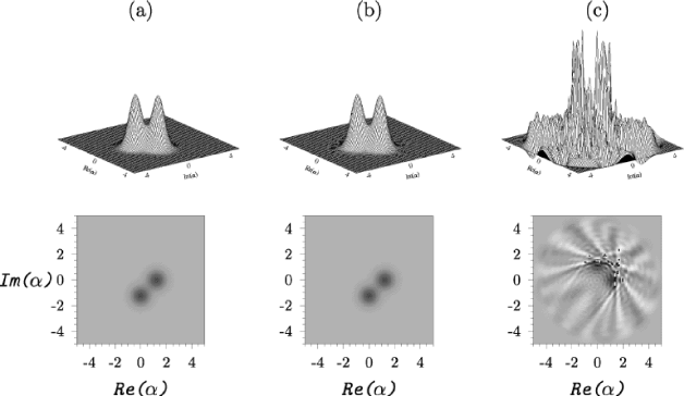
FIG. 6.: Wigner function of an incoherent superposition of two coherent states (a), its reconstruction via the maximum entropy principle (b) and its reconstruction via projection onto pattern functions (c). The upper line shows the Wigner function as surface plots, whereas the lower line shows the same functions as a grey scale plot, where dark areas correspond to higher values and bright areas to lower values. We see that the reconstruction via the MaxEnt principle is much more reliable then a straightforward application of direct sampling via pattern functions.

TABLE I.: Deviation $\Delta$ of the reconstructed state from the incoherent superposition of two coherent states for reconstruction via the maximum entropy principle and for reconstruction via projection onto pattern functions.

One might suspect that the superiority of the reconstruction via the maximum entropy principle might be a speciality of the selected state, an incoherent superposition of two coherent states. Therefore we want to give some more examples, e.g. the corresponding coherent superposition, as defined in (274). As in the previous example the values of $\alpha_{1}$ and $\alpha_{2}$ were chosen to be $1.25$ and $1.25\,i$, respectively (see Fig.7).

Surprisingly enough the reconstruction turns out to be simplified by the quantum interferences apparent in the cat state: the deviations for both reconstruction schemes are smaller than for the incoherent superposition (Table II). Apart from this the overall picture remains the same: The reconstruction with the maximum entropy principle is many orders of magnitudes better than the reconstruction via pattern functions. Moreover, the reconstruction via pattern functions may again result in density operators which are not positive definite.

Next, we discuss the reconstruction of the rectangular state as defined in (275). Though this state is of less relevance in quantum optics it can be easily realized for atomic beams by an aperture. The reason, why we include this state into our discussion is twofold: on one hand, the oscillations in its Wigner function (see below) represent a serious difficulty for quantum tomography, so it is interesting to check, whether other reconstruction schemes do not have this difficulty. On the other hand the smoothening character of our reconstruction by selecting the state with maximum entropy may smooth out just these oscillations and therefore this state is a critical test of the maximum entropy reconstruction.

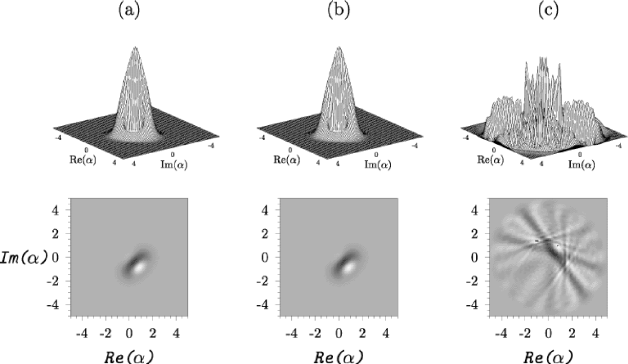
FIG. 7.: Wigner function of a coherent superposition of two coherent states given by Eq.(274) (a), its reconstruction via the maximum entropy principle (b) and its reconstruction via the projection onto pattern functions (c). Again the upper line shows the state as surface plot and the lower line the corresponding grey scale plots.

TABLE II.: Deviation $\Delta$ of the reconstructed state from the coherent superposition of two coherent states for reconstruction via the maximum entropy principle and for reconstruction via projection onto pattern functions.

The overall picture (Fig. 8) is the same as for the previous two examples: the reconstruction via the maximum entropy principle gives a deviation (see also Table III) from the original state many orders of magnitude lower than conventional quantum tomography does. Once more we want to stress that the bad reconstruction by usual quantum tomography is due to the extremely small number of angles and grid points. Increasing the amount of measurement data makes this reconstruction scheme working.

Finally, we turn to a state, which is relatively easy to reconstruct via quantum tomography: a number state (277) with $n=4$. This state can be obtained even exactly with a finite number of phases $N_{\theta}$ provided that $N_{\theta}=n+1$ and that each quadrature is measured completely, i.e. covering densely the whole axis. Since our examples do not and cannot fulfill the latter condition, we encounter again a situation where the reconstruction via quantum tomography suffers from too few measurement data. To allow for a fair comparison we restrict the Hilbert space to $N=n=4$, otherwise quantum tomography adds additional errors in the higher density matrix elements.

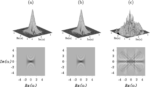
FIG. 8.: Wigner function of a rectangular state given by [see Eq.(275)] (a), its reconstruction via the maximum entropy principle (b) and its reconstruction via the projection onto pattern functions (c).

TABLE III.: Deviation $\Delta$ of the reconstructed state from the rectangular state for reconstruction via the maximum entropy principle and for reconstruction via projection onto pattern functions.

All errors (Table IV) are smaller than their counterparts for the other states considered so far, which is also due to the smaller Hilbert space under consideration. For this state the conventional reconstruction also gives a very good estimate of the state (see Fig. 9), though the absolute values of the oscillations in the Wigner function (Fig. 9) are not completely correct due to the finite number of measurements on each axis. But even for this state, which is advantageous for quantum tomography, the errors of the reconstruction via the maximum entropy principle are much smaller.

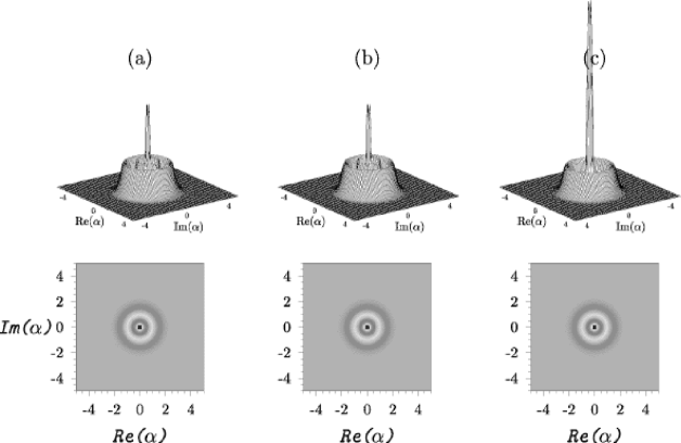
FIG. 9.: Wigner function of a Fock state (a), its reconstruction via the maximum entropy principle (b) and its reconstruction via the projection onto pattern functions (c).

TABLE IV.: Deviation $\Delta$ of the reconstructed state from the Fock state for reconstruction via the maximum entropy principle and for reconstruction via projection onto pattern functions.

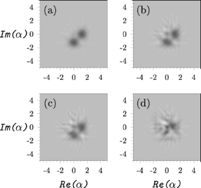
FIG. 10.: Wigner function as grey-scale plots of the reconstruction of the incoherent superposition shown in Fig. 6. Here we assume measurement results with errors. The errors are proportional to a factor $\eta$, which is $10^{-2}$ (a), $5\cdot 10^{-2}$ (b), $10^{-1}$ (c) and $5\cdot 10^{-1}$ (d).

B Measurement errors and incompatible measurement results

We want to discuss briefly the influence of measurement errors. Including measurement errors we encounter a new problem: we cannot guarantee that there is any state with positive definite density matrix compatible with all measurement results (8). In other words, the set ${\cal C}$ as defined by Eq. (8) is empty. Practically this means that our numerical procedure to solve numerically the equations for the Lagrange parameters cannot converge. Fortunately it turns out that the set of Lagrange parameters minimizing the deviation

$$\left(\bar{n}-{\rm Tr}\left\{\tilde{\rho}\hat{n}\right\}\right)^{2}+\sum_{lm}\left(o^{\prime}_{lm}-{\rm Tr}\left\{\tilde{\rho}\hat{O}_{lm}\right\}\right)^{2}$$ (281)

gives generally an excellent estimate for the state to be reconstructed. To illustrate this we take our state and spoil artificially our measurement results by

$$o^{\prime}_{lm}=o_{lm}+\eta\xi_{lm}\sqrt{o_{lm}}.$$ (282)

$o^{\prime}_{lm}$ is the result of the measurement with errors, whereas $o_{lm}={\rm Tr}(\hat{\rho}\hat{O}_{lm})$ is the corresponding result one would obtain in an ideal measurement. The error was chosen to be proportional to the square root of $o_{lm}$ since this quantity is obtained by measuring $x_{\theta}$ several times and counting how much results fall into a certain interval. The proportionality factor $\eta$ characterizes the quality of our measurement and depends on the number of single measurements made. $\xi_{lm}$ represent independent Gaussian random numbers with

$$\langle\xi_{lm}\rangle = 0$$ (283)

$$\langle\xi_{lm}\xi_{l^{\prime}m^{\prime}}\rangle = \delta_{ll^{\prime}}\delta_{mm^{\prime}}.$$ (284)

FIG. 11.: Wigner function as grey-scale plots of the reconstruction of the cat state shown in Fig. 7 on the basis of measurement results with errors. The errors are proportional to a factor $\eta$, which is $10^{-2}$ (a), $5\cdot 10^{-2}$ (b), $10^{-1}$ (c) and $5\cdot 10^{-1}$ (d).

With these $o_{lm}$ and various parameters $\eta$ we started again the reconstruction of the incoherent superposition (273), the cat state (274), the rectangular state and the Fock state already discussed in the last paragraph. For all reconstructions we used $N_{\theta}=4$ different axis’ and $N_{x}=13$ points at each axis, covering the interval $[-2,2]$ as before.

Fig. 10 shows the Wigner functions of the reconstruction of the incoherent superposition for $\eta=10^{-2}$, $5\cdot 10^{-2}$, $10^{-1}$ and $5\cdot 10^{-1}$. Despite the relative large values of $\eta$—corresponding to a large error—the reconstruction is very good. We also calculated the error as defined in (280) and obtained $\Delta=4\cdot 10^{-3}$ for $\eta=10^{-2}$, $\Delta=4\cdot 10^{-2}$ for $\eta=5\cdot 10^{-2}$, $\Delta=5\cdot 10^{-2}$ for $\eta=0.1$ and $\Delta=0.3$ for $\eta=0.5$. For $\eta=0.05$ we recognize a slight asymmetry between the two spots, which becomes more pronounced for the highest value of $\eta$. But still the two dots are easily distinguishable. Due to the random character of our calculation these numbers will vary when varying the random numbers—as the results of a measurements will vary from run to run.

Next, we present the corresponding plots for the cat state (Fig. 11). As in the previous figure the values for $\eta$ are $10^{-2}$, $5\cdot 10^{-2}$, $10^{-1}$ and $5\cdot 10^{-1}$ for (a), (b), (c) and (d), respectively. The obtained errors $\Delta$ are $3\cdot 10^{-3}$, $3\cdot 10^{-2}$, $7\cdot 10^{-2}$ and $2\cdot 10^{-1}$. We want to emphasize that for both states even for the largest value of $\eta$ the reconstruction is better than the usual quantum tomography without errors.

Now we discuss the influence of measurement errors for the rectangular state. Fig. 12 shows the Wigner functions of the reconstruction with an error parameter $\eta=10^{-2}$ (a), $5\cdot 10^{-2}$ (b), $10^{-1}$ (c) and $5\cdot 10^{-1}$ (d). As for the previous states only for the highest error parameter $\eta$ we recognize an asymmetry not present in the original state (Fig. 8 (a)). The resulting errors were $2\cdot 10^{-3}$, $2\cdot 10^{-2}$, $6\cdot 10^{-2}$ and $3\cdot 10^{-1}$, respectively. Despite the relatively large errors the reconstruction is as in the previous examples very good. Only for the largest value of $\eta$ we recognize a qualitative difference to the original state Fig. 8 (a).

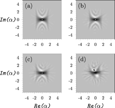
FIG. 12.: Wigner function as grey-scale plots of the reconstruction of the rectangular state shown in Fig. 8 on the basis of measurement results with errors. The errors are proportional to a factor $\eta$, which is $10^{-2}$ (a), $5\cdot 10^{-2}$ (b), $10^{-1}$ (c) and $5\cdot 10^{-1}$ (d).

FIG. 13.: Wigner function as grey-scale plots of the reconstruction of the Fock state shown in Fig. 9 on the basis of measurement results with errors. The errors are proportional to a factor $\eta$, which is $10^{-2}$ (a), $5\cdot 10^{-2}$ (b), $10^{-1}$ (c) and $5\cdot 10^{-1}$ (d).

Finally, we turn to the influence of measurement errors on the reconstruction of the Fock state. The errors $\Delta$ for the various error parameters $\eta$ are $\Delta=8\cdot 10^{-4}$ for $\eta=1\cdot 10^{-2}$, $\Delta=1\cdot 10^{-2}$ for $\eta=5\cdot 10^{-2}$, $\Delta=4\cdot 10^{-2}$ for $\eta=0.1$, and $\Delta=0.7$ for $\eta=0.5$. Also the plots of the corresponding Wigner functions (Fig. 13) reveal that the reconstruction is very good and shows the ring-shaped structure of the original Fig. 9 (a). Only for the $\eta=0.5$ the reconstruction is not good enough to show clearly this feature.

Usually this kind of measurement results into a very good reconstruction of Wigner functions (such that the corresponding entropy is close to zero for pure states). Nevertheless, a certain attention has to be paid for highly squeezed states, such as the Vogel-Schleich phase states [69], for which the measurement of distributions $w_{\hat{\rho}}(x_{\theta_{j}})$ can be problematic. Namely, $w_{\hat{\rho}}(x_{\theta_{j}})$ can be very “wide”, so that the normalization condition is not fulfilled in a domain of physically accessible values of $x_{\theta_{j}}$.

In this Section we have presented a numerical application of the reconstruction scheme via the MaxEnt principle for a reconstruction of Wigner functions of quantum-mechanical states of light from incomplete tomographic data. We have shown that when the tomographic data are incomplete, then the reconstruction via the MaxEnt principle is much more reliable than the standard inversion Radon transformation scheme or the pattern-function scheme.

VII RECONSTRUCTION OF SPIN STATES VIA MAXENT PRINCIPLE

In the following sections we will apply the Jaynes principle for the reconstruction of pure spin states (see also [70]). Firstly, for illustrative purposes we present the simple example of the reconstruction of states of a single spin-1/2 system with the help of the maximum-entropy principle. Then we will discuss the partial reconstruction of entangled spin states. In particular, we will analyze the problem how to identify incomplete observation levels on which the complete reconstruction can be performed for the Bell and the Greenberger–Horne–Zeilinger states (i.e., the corresponding entropy is equal to zero and the generalized canonical density operator is identical to $\hat{\rho}_{0}$).

A Single spin-1/2

Firstly we illustrate the application of the maximum-entropy principle for the partial quantum–state reconstruction of single spin–$1/2$ system. Let us consider an ensemble of spins-$1/2$ in an unknown pure state $|\psi_{0}\rangle$. In the most general case this unknown state vector $|\psi_{0}\rangle$ can be parameterized as

$$|\psi_{0}\rangle=\cos\theta/2|1\rangle+\mbox{e}^{i\varphi}\sin\theta/2|0\rangle,$$ (285)

where $|0\rangle$, $|1\rangle$ are eigenstates of the $z$-component of the spin operator $\hat{s}_{z}={1\over 2}\hat{\sigma}_{z}$ with eigenvalues $-{1\over 2}$, ${1\over 2}$, respectively. The corresponding density operator $\hat{\rho}_{0}=|\psi_{0}\rangle\langle\psi_{0}|$ can be written in the form

$$\hat{\rho}_{0}={1\over 2}\left(\hat{I}+\vec{n}.\hat{\vec{\sigma}}\right),$$ (286)

where $\hat{I}$ is the unity operator, $\vec{n}=(\sin\theta\cos\varphi,\sin\theta\sin\varphi,\cos\theta)$; $\hat{\vec{\sigma}}=(\hat{\sigma}_{x},\hat{\sigma}_{y},\hat{\sigma}_{z})$ are the Pauli spin operators which in the matrix representation in the basis $|0\rangle$, $|1\rangle$ read

$$\hat{\sigma}_{x}=\left(\begin{array}[]{cc}0&1\\ 1&0\end{array}\right),\quad\hat{\sigma}_{y}=\left(\begin{array}[]{cc}0&-i\\ i&0\end{array}\right),\quad\hat{\sigma}_{z}=\left(\begin{array}[]{cc}1&0\\ 0&-1\end{array}\right).$$ (293)

TABLE V.: In this table we present three observation levels ${\cal O}_{\rm A}^{(1)}$; ${\cal O}_{\rm B}^{(1)}$, and ${\cal O}_{\rm comp}^{(1)}$ associated with a measurement of the particular spin-1/2 operators. Bullets ($\bullet$) in the table indicate which observables constitute a given observation level. We also present explicit expressions for the reconstructed density operators $\hat{\rho}_{\rm A}$; $\hat{\rho}_{\rm B}$ and $\hat{\rho}_{\rm comp}$.

To determine completely the unknown state one has to measure three linearly independent (e.g., orthogonal) projections of the spin. After the measurement of the expectation value of each observable, a reconstruction of the generalized canonical density operator (12) according to the maximum-entropy principle can be performed. In Table V we consider three observation levels defined as ${\cal O}_{A}^{(1)}=\{\hat{\sigma}_{z}\}$, ${\cal O}_{B}^{(1)}=\{\hat{\sigma}_{z},\hat{\sigma}_{x}\}$ and ${\cal O}_{C}^{(1)}=\{\hat{\sigma}_{z},\hat{\sigma}_{x},\hat{\sigma}_{y}\}\equiv{\cal O}_{comp}$ [the superscript of the observation levels indicates the number of spins–$1/2$ under consideration].

Using algebraic properties of the $\hat{\sigma}_{\nu}$-operators, the generalized canonical density operator (12) can be expressed as

$$\hat{\rho}_{\cal O}={1\over Z}\exp(-\vec{\lambda}.\hat{\vec{\sigma}})={1\over Z}\left[\cosh|\lambda|\hat{I}-\sinh|\lambda|{\vec{\lambda}.\hat{\vec{\sigma}}\over|\lambda|}\right],\qquad Z=2\cosh|\lambda|,$$ (294)

with $\vec{\lambda}=(\lambda_{x},\lambda_{y},\lambda_{x})$ and $|\lambda|^{2}=\lambda_{x}^{2}+\lambda_{y}^{2}+\lambda_{z}^{2}$. The final form of the $\hat{\rho}_{\cal O}$ on particular observation levels is given in Table V. The corresponding entropies can be written as

$$S_{\cal O}=-p_{\cal O}\ln p_{\cal O}-(1-p_{\cal O})\ln(1-p_{\cal O}),$$ (295)

where $p_{\cal O}$ is one eigenvalue of $\hat{\rho}_{\cal O}$ [the other eigenvalue is equal to $(1-p_{\cal O})$] which reads as

$$p_{A}={1+|\langle\hat{\sigma}_{z}\rangle|\over 2},\quad p_{B}={1+\sqrt{\langle\hat{\sigma}_{x}\rangle^{2}+\langle\hat{\sigma}_{z}\rangle^{2}}\over 2},\quad p_{\rm comp}={1+\sqrt{\langle\hat{\sigma}_{x}\rangle^{2}+\langle\hat{\sigma}_{y}\rangle^{2}+\langle\hat{\sigma}_{z}\rangle^{2}}\over 2}.$$ (296)

It is seen that the entropy $S_{\cal O}$ is equal to zero if and only if $p_{\cal O}=1$. From here follows that on ${\cal O}_{A}^{(1)}$ only the basis vectors $|0\rangle$ and $|1\rangle$ with $|\langle\hat{\sigma}_{z}\rangle|=1$ can be fully reconstructed. Nontrivial is ${\cal O}_{B}^{(1)}$, on which a whole set of pure states (285) with $\langle\hat{\sigma}_{y}\rangle=0$ (i.e., $\varphi=0$) can be uniquely determined. For such states $S_{B}=0$ and further measurement of the $\hat{\sigma}_{y}$ on ${\cal O}_{comp}$ represents redundant (useless) information.

B Two spins–1/2

Now we assume a system composed of two distinguishable spins–$1/2$. If we are performing only local measurements of observables such as $\hat{\sigma}_{\mu}^{(1)}\otimes\hat{I}^{(2)}$ and $\hat{I}^{(1)}\otimes\hat{\sigma}_{\nu}^{(2)}$ (here superscripts label the particles) which do not reflect correlations between the particles then the reconstruction of the density operator reduces to an estimation of individual (uncorrelated) spins–1/2, i.e., the reconstruction reduces to the problem discussed in the previous section. For each spin–$1/2$ the reconstruction can be performed separately and the resulting generalized canonical density operator is given as a tensor product of particular generalized canonical density operators, i.e., $\hat{\rho}=\hat{\rho}^{(1)}\otimes\hat{\rho}^{(2)}$. In this case just the uncorrelated states $|\psi_{0}\rangle=|\psi_{0}^{(1)}\rangle\otimes|\psi_{0}^{(2)}\rangle$ can be fully reconstructed. Nevertheless, the correlated (nonfactorable) states $|\psi_{0}\rangle\neq|\psi_{0}^{(1)}\rangle\otimes|\psi_{0}^{(2)}\rangle$ are of central interest.

TABLE VI.: We present a set of observation levels on which the density operators of two spins-1/2 can be partially reconstructed. Bullets ($\bullet$) in the table indicate which observables constitute a given observation level while empty circles ($\circ$) denote unmeasured observables (i.e., these observables are not included in the given observation level) for which the maximum-entropy principle ‘predicts” nonzero mean values.

In general, any density operator of a system composed of two distinguishable spins–$1/2$ can be represented by a $4\times 4$ Hermitian matrix and $15$ independent numbers are required for its complete determination. It is worth noticing that $15$ operators (observables)

$$\{\hat{\sigma_{\mu}}^{(1)}\otimes\hat{I}^{(2)},\hat{I}^{(1)}\otimes\hat{\sigma_{\nu}}^{(2)},\hat{\sigma}_{\mu}^{(1)}\otimes\hat{\sigma}_{\nu}^{(2)}\};\qquad(\mu,\nu=x,y,z),$$ (297)

together with the identity operator $\hat{I}^{(1)}\otimes\hat{I}^{(2)}$ form an operator algebra basis in which any operator can be expressed. In this “operator” basis each density operator can be written as

$$\hat{\rho}={1\over 4}\left[\hat{I}^{(1)}\otimes\hat{I}^{(2)}+\vec{n}^{(1)}.~{}\hat{\vec{\sigma}}^{(1)}\otimes\hat{I}^{(2)}+\vec{n}^{(2)}.~{}\hat{I}^{(1)}\otimes\hat{\vec{\sigma}}^{(2)}+\sum_{\mu,\nu}\xi_{\mu\nu}\hat{\sigma}_{\mu}^{(1)}\otimes\hat{\sigma}_{\nu}^{(2)}\right],$$ (298)

with $\xi_{\mu\nu}=\langle\hat{\sigma}_{\mu}^{(1)}\otimes\hat{\sigma}_{\nu}^{(2)}\rangle$ ($\mu,\nu=x,y,z$).

Using the maximum-entropy principle we can (partially) reconstruct an unknown density operator $\hat{\rho}_{0}$ on various observation levels. Conceptually the method of maximum entropy is rather straightforward: one has to express the generalized canonical density operator (12) for two spins-1/2 in the form (298) from which a set of nonlinear equations for Lagrange multipliers $\lambda_{\nu}$ is obtained.

Due to algebraic properties of the operators under the consideration the practical realization of this programme can be technically difficult (see Appendix A). In Table VI we define some nontrivial observation levels. Measured observables which define a particular observation level are indicated in Table VI by bullets ($\bullet$) while the empty circles ($\circ$) indicate unmeasured observables (i.e., these observables are not included in the given observation level) for which the maximum-entropy principle “predicts” nonzero mean values. This means that the maximum-entropy principle provide us with a nontrivial estimation of mean values of unmeasured observables. The generalized canonical density operators which correspond to the observation levels considered in Table VI are presented in Table VII. The signs “$\oplus,\ominus$” are used to indicate unmeasured observables for which nontrivial information can be obtained with the help of the maximum-entropy principle.

TABLE VII.: We present explicit expressions for the reconstructed density operators $\hat{\rho}_{\rm X}$ of two spins-1/2 on the observation levels denoted in Table 2. We use the notation $n_{\mu}^{(p)}=\langle\hat{\sigma}_{\mu}^{(p)}\rangle$ ($\mu=z,x,y;\quad p=1,2$) and $\xi_{\mu\nu}=\langle\hat{\sigma}_{\mu}^{(1)}\otimes\hat{\sigma}_{\nu}^{(2)}\rangle$ with $\mu,\nu=z,x,y$. The signs $\oplus$ and $\ominus$ are used to indicate unmeasured observables for which nontrivial information can be obtained with the help of the maximum-entropy principle.

C Reconstruction of Bell states

In what follows we analyze a partial reconstruction of the Bell states (i.e., the most correlated two particle states) on observation levels given in Table VI. One of our main tasks will be to find the minimum observation level (i.e., the set of system observables) on which the complete reconstruction of these states can be performed. Obviously, if all 15 observables are measured, then any state of two spins-1/2 can be reconstructed precisely. Nevertheless, due to the quantum entanglement between the two particles, measurements of some observables will simply be redundant. To find the minimal set of observables which uniquely determine the Bell state one has to perform either a sequence of reductions of the complete observation level, or a systematic extension of the most trivial observation level ${\cal O}^{(2)}_{A}$.

Let us consider particular examples of Bell states, of the form

$$|\Psi_{\varphi}^{(Bell)}\rangle={1\over\sqrt{2}}\left[|1,1\rangle+\mbox{e}^{i\varphi}|0,0\rangle\right],\quad\hat{\rho}_{\varphi}^{(Bell)}=|\Psi_{\varphi}^{(Bell)}\rangle\langle\Psi_{\varphi}^{(Bell)}|,$$ (299)

(other Bell states are discussed later). These maximally correlated states have the property that the result of a measurement performed on one of the two spins–$1/2$ uniquely determines the state of the second spin. Therefore, these states find their applications in quantum communication systems [23, 52]. In addition, they are suitable for testing fundamental principles of quantum mechanics [1] such as the complementarity principle or local hidden–variable theories [71].

Let us analyze now a sequence of successive extensions of the observation level ${\cal O}_{A}^{(2)}$

$${\cal O}_{A}^{(2)}\subset{\cal O}_{B}^{(2)}\subset{\cal O}_{C}^{(2)}\subset{\cal O}_{D}^{(2)}.$$ (300)

The observation level ${\cal O}_{A}^{(2)}$ (see Table VI) is associated with the measurement of $\hat{\sigma}_{z}$ observables of each spin individually, i.e., it is insensitive with respect to correlations between the spins. On ${\cal O}_{B}^{(2)}$ both $z$-spin components of particular spins and their correlation have been recorded (simultaneous measurement of these observables is possible because they commute). Further extension to the observation level on ${\cal O}_{C}^{(2)}$ corresponds to a rotation of the Stern–Gerlach apparatus such that the $x$-spin component of the second spin–$1/2$ is measured. The observation level ${\cal O}_{D}^{(2)}$ is associated with another rotation of the Stern–Gerlach apparatus which would allow us to measure the $y$-spin component. The generalized canonical density operators on the observation levels ${\cal O}_{B}^{(2)}$, ${\cal O}_{C}^{(2)}$ and ${\cal O}_{D}^{(2)}$ predict zero mean values for all the unmeasured observables (297) (see Table VII).

In general, successive extensions (300) of the observation level ${\cal O}_{A}^{(2)}$ should be accompanied by a decrease in the entropy of the reconstructed state which should reflect increase of our knowledge about the quantum-mechanical system under consideration. Nevertheless, we note that there are states for which the entropy remains constant when ${\cal O}_{B}^{(2)}$ is extended towards ${\cal O}_{C}^{(2)}$ and ${\cal O}_{D}^{(2)}$, i.e., the performed measurements are in fact redundant. For instance, this is the case for the maximally correlated state (299). Here entropies associated with given observation levels read

$$S_{A}=2\ln 2,\qquad S_{B}=S_{C}=S_{D}=\ln 2,$$ (301)

respectively, which mean that these observation levels are not suitable for reconstruction of the Bell states. The reason is that the Bell states have no “preferable” direction for each individual spin, i.e., $\langle\hat{\sigma}_{\mu}^{(p)}\rangle=0$ for $\mu=x,y,z$ and $p=1,2$.

From the above it follows that, for a nontrivial reconstruction of Bell states, the observables which reflect correlations between composite spins also have to be included into the observation level. Therefore let us now discuss the sequence of observation levels

$${\cal O}_{E}^{(2)}\subset{\cal O}_{F}^{(2)}\subset{\cal O}_{G}^{(2)}$$ (302)

associated with simultaneous measurement of spin components of the two particles [see Table VI]. The corresponding generalized canonical density operators are given in Table VII. To answer the question of which states can be completely reconstructed on the observation level ${\cal O}_{E}^{(2)}$ we evaluate the von Neumann entropy of the generalized canonical density operator $\hat{\rho}_{E}$. For the Bell states we find that $S_{E}=-p_{E}\ln p_{E}-(1-p_{E})\ln(1-p_{E})$ where $p_{E}=(1-\cos\varphi)/2$. We can also compare directly $\hat{\rho}_{\varphi}^{(Bell)}$ with $\hat{\rho}_{E}$. The density operator $\hat{\rho}_{\varphi}^{(Bell)}$ in the matrix form can be written as

$$\hat{\rho}_{\varphi}^{(Bell)}={1\over 2}\left(\begin{array}[]{cccc}1&0&0&\mbox{e}^{-i\varphi}\\ 0&0&0&0\\ 0&0&0&0\\ \mbox{e}^{i\varphi}&0&0&1\end{array}\right),$$ (307)

while the corresponding operator reconstructed on the observation level ${\cal O}_{E}^{(2)}$ reads

$$\hat{\rho}_{E}={1\over 2}\left(\begin{array}[]{cccc}1&0&0&\cos\varphi\\ 0&0&0&0\\ 0&0&0&0\\ \cos\varphi&0&0&1\end{array}\right).$$ (312)

We see that $\hat{\rho}_{\varphi}^{(Bell)}=\hat{\rho}_{E}$ and $S[\hat{\rho}_{E}]=0$ only if $\varphi=0$ or $\pi$ which means that the Bell states $|\Psi_{\varphi=0,\pi}\rangle={1\over\sqrt{2}}\left[|1,1\rangle\pm|0,0\rangle\right]$ are completely determined by mean values of two observables $\hat{\sigma}_{z}^{(1)}\otimes\hat{\sigma}_{z}^{(2)}$ and $\hat{\sigma}_{x}^{(1)}\otimes\hat{\sigma}_{x}^{(2)}$ and that these states can be completely reconstructed on ${\cal O}_{E}^{(2)}$. We note that two other maximally correlated states $|\Phi_{\pm}\rangle={1\over\sqrt{2}}\left[|0,1\rangle\pm|1,0\rangle\right]$ can also be completely reconstructed on ${\cal O}_{E}^{(2)}$.

The extension of ${\cal O}_{E}^{(2)}$ to ${\cal O}_{F}^{(2)}$ does not increase the amount of information about the Bell states (299) with $\varphi\neq 0,\pi$. For this reason we have to consider further extension of ${\cal O}_{F}^{(2)}$ to the observation level ${\cal O}_{G}^{(2)}$ (see Table VI and Appendix A). In what follows we will show that this is an observation level on which all Bell states (299) can be completely reconstructed. To see this one has to realize two facts. Firstly, the generalized canonical density operator $\hat{\rho}_{G}$ given by Eq.(12) can be expressed as a linear superposition of observables associated with the given observation level, i.e.:

$$\hat{\rho}_{G}=\frac{1}{Z_{G}}\exp\left(-\sum_{\mu=x,y,z}\lambda_{\mu\mu}\hat{\sigma}_{\mu}^{(1)}\otimes\hat{\sigma}_{\mu}^{(2)}-\lambda_{xy}\hat{\sigma}_{x}^{(1)}\otimes\hat{\sigma}_{y}^{(2)}-\lambda_{yx}\hat{\sigma}_{y}^{(1)}\otimes\hat{\sigma}_{x}^{(2)}\right)$$ (313)

$$=\frac{1}{4}\left(\hat{1}-\sum_{\mu=x,y,z}\xi_{\mu\mu}\hat{\sigma}_{\mu}^{(1)}\otimes\hat{\sigma}_{\mu}^{(2)}-\xi_{xy}\hat{\sigma}_{x}^{(1)}\otimes\hat{\sigma}_{y}^{(2)}-\xi_{yx}\hat{\sigma}_{y}^{(1)}\otimes\hat{\sigma}_{x}^{(2)}\right),$$ (314)

where the parameters $\xi_{\mu\nu}$ are functions of the Lagrange multipliers $\lambda_{\mu\nu}$. Secondly, for Bell states (299) the only observables which have nonzero expectation values are those associated with ${\cal O}_{G}^{(2)}$. Namely, $\langle\hat{\sigma}_{z}^{(1)}\otimes\hat{\sigma}_{z}^{(2)}\rangle=1$, $\langle\hat{\sigma}_{x}^{(1)}\otimes\hat{\sigma}_{x}^{(2)}\rangle=-\langle\hat{\sigma}_{y}^{(1)}\otimes\hat{\sigma}_{y}^{(2)}\rangle=\cos\varphi$ and $\langle\hat{\sigma}_{x}^{(1)}\otimes\hat{\sigma}_{y}^{(2)}\rangle=\langle\hat{\sigma}_{y}^{(1)}\otimes\hat{\sigma}_{x}^{(2)}\rangle=\sin\varphi$. It means that all coefficients in the generalized canonical density operator $\hat{\rho}_{G}$ given by Eq. (298) are uniquely determined by the measurement, i.e., $\hat{\rho}_{G}=\hat{\rho}_{\varphi}$.

From the above it follows that Bell states can be completely reconstructed on the observation level ${\cal O}_{G}^{(2)}$. On the other hand, ${\cal O}_{G}^{(2)}$ is not the minimum observation level on which these states can be completely reconstructed. The minimum set of observables which would allow us to reconstruct Bell states uniquely can be found by a reduction of ${\cal O}_{G}^{(2)}$. Direct inspection of a finite number of possible reductions reveals that Bell states can be completely reconstructed on those observation level which can be obtained from ${\cal O}_{G}^{(2)}$ when one of the observables $\hat{\sigma}_{\nu}^{(1)}\otimes\hat{\sigma}_{\nu}^{(2)}$ ($\nu=x,y,z$) is omitted. As an example, let us consider the observation level ${\cal O}_{H}^{(2)}$ given in Table VI which represents a reduction of ${\cal O}_{G}^{(2)}$ when the observable $\hat{\sigma}_{z}^{(1)}\otimes\hat{\sigma}_{z}^{(2)}$ is omitted. Performing the Taylor series expansion of the generalized canonical density operator $\hat{\rho}_{H}$ defined by Eq. (() ‣ A. 2. Observation level ${\cal O}_{H}^{(2)}$) one can find that the only new observable $\hat{\sigma}_{z}^{(1)}\otimes\hat{\sigma}_{z}^{(2)}$ enters the expression for the $\hat{\rho}_{H}$ as indicated in Table VII. The coefficient $t$ in front of $\hat{\sigma}_{z}^{(1)}\otimes\hat{\sigma}_{z}^{(2)}$ can either be found explicitly in a closed analytical form (see Appendix A) or can be obtained from the following variational problem. Namely, we remind ourselves that the expression (() ‣ A. 2. Observation level ${\cal O}_{H}^{(2)}$) for $\hat{\rho}_{H}$ helps us to identify those unmeasured observables for which the Jaynes principle of the maximum entropy “predicts” nonzero mean values. At this stage we still have to find the particular value of the parameter $t$ for which the density operator $\hat{\rho}_{H}$ in Table VII leads to the maximum of the von Neumann entropy. To do so we search through the one-dimensional parametric space which is bounded as $-1\leq t\leq 1$. To be specific, first of all, for $t\in\langle-1,1\rangle$ we have to exclude those operators which are not true density operators (i.e., any such operators which have negative eigenvalues). Then we “pick” up from a physical parametric subspace the generalized canonical density operator with the maximum von Neumann entropy. Direct calculation for Bell states shows that the physical parametric subspace is reduced to an isolated “point” with $t=\langle\hat{\sigma}_{z}^{(1)}\otimes\hat{\sigma}_{z}^{(2)}\rangle=1$. Therefore we conclude that Bell states can completely be reconstructed on ${\cal O}_{H}$. Two other minimum observation levels suitable for the complete reconstruction of Bell states can be obtained by a reduction of ${\cal O}_{G}^{(2)}$ when either $\hat{\sigma}_{x}^{(1)}\otimes\hat{\sigma}_{x}^{(2)}$ or $\hat{\sigma}_{y}^{(1)}\otimes\hat{\sigma}_{y}^{(2)}$ is omitted. On the other hand, direct inspection shows that a reduction of ${\cal O}_{G}^{(2)}$ by exclusion of either $\hat{\sigma}_{x}^{(1)}\otimes\hat{\sigma}_{y}^{(2)}$ or $\hat{\sigma}_{y}^{(1)}\otimes\hat{\sigma}_{z}^{(2)}$ leads to an incomplete observation level with respect to Bell states.

In what follows we discuss briefly two other observation levels ${\cal O}_{I}^{(2)}$ and ${\cal O}_{J}^{(2)}$ which are defined in Table VI. The observation level ${\cal O}_{I}^{(2)}$ serves as an example when one can find an analytical expression for the Taylor series expansion of the canonical density operator $\hat{\rho}_{I}$ (see Table VII) in the form (298). The coefficients (functions of the original Lagrange multipliers) in front of particular observables in Eq.(298) can be identified and are given in Table VII. Problems do appear when ${\cal O}_{I}^{(2)}$ is extended towards ${\cal O}_{J}^{(2)}$. In this case we cannot simplify the exponential expression for $\hat{\rho}_{J}$ and rewrite it analytically in the form (298) as a linear combination of the observables (297). In this situation one should apply the following procedure: firstly, by performing the Taylor-series expansion of the $\hat{\rho}_{J}$ to the lowest orders one can identify the observables with nonzero coefficients in the form (298). Namely, for $\hat{\rho}_{J}$ the additional observables $\hat{\sigma}_{z}^{(1)}\otimes\hat{\sigma}_{x}^{(2)}$, $\hat{\sigma}_{x}^{(1)}\otimes\hat{\sigma}_{z}^{(2)}$ and $\hat{\sigma}_{y}^{(1)}\otimes\hat{\sigma}_{y}^{(2)}$ appear in addition to those which form ${\cal O}_{H}^{(2)}$ [see Table VII]. The corresponding coefficients $u,v,w\in\langle-1,1\rangle$ form a bounded three–dimensional parametric space $(u,v,w)$. In the second step one can use constructively the maximum-entropy principle to choose within this parametric space the density operator with the maximum von Neumann entropy. The basic procedure is to scan the whole three–dimensional parametric space. At the beginning, one has to select out those density operators (i.e., those parameters $u,v,w$) which posses negative eigenvalues and do not represent genuine density operators. Finally, from a remaining set of “physical” density operators which are semi–positively defined the canonical density operator $\hat{\rho}_{J}$ with maximum von Neumann entropy has to be chosen. For a completeness, let us notice that for Bell states the observation levels ${\cal O}_{I}^{(2)}$ and ${\cal O}_{J}^{(2)}$ are equivalent to ${\cal O}_{E}^{(2)}$, i.e., $\hat{\rho}_{I}=\hat{\rho}_{J}=\hat{\rho}_{E}$.

In this section we have found the minimum observation levels [e.g., ${\cal O}_{H}^{(2)}$] which are suitable for the complete reconstruction of Bell states. These observation levels are associated with the measurement of two–spin correlations $\hat{\sigma}_{x}^{(1)}\otimes\hat{\sigma}_{z}^{(2)}$, $\hat{\sigma}_{y}^{(1)}\otimes\hat{\sigma}_{z}^{(2)}$ and two of the observables $\hat{\sigma}_{\nu}^{(1)}\otimes\hat{\sigma}_{\nu}^{(2)}$ ($\nu=x,y,z$). Once this problem has been solved, it is interesting then to find a minimum set of observables suitable for a complete reconstruction of maximally correlated spin states systems consisting of more than two spins–$1/2$. In the following section we will investigate the (partial) reconstruction of Greenberger-Horne-Zeilinger states of three spins–1/2 on various observation levels.

D Three spins–1/2

Even though the Jaynes principle of maximum entropy provides us with general instructions on how to reconstruct density operators of quantum-mechanical systems practical applications of this reconstruction scheme may face serious difficulties. In many cases the reconstruction scheme fails due to insurmountable technical problems (e.g. the system of equations for Lagrange multipliers cannot be solved explicitly). We have illustrated these problems in the previous section when we have discussed the reconstruction of a density operator of two spins–1/2. Obviously, the general problem of reconstruction of density operators describing a system composed of three spins–1/2 is much more difficult. Nevertheless a (partial) reconstruction of some states of this system can be performed. In particular, in this section we will discuss a reconstruction of the maximally correlated three spin-1/2 states – the so-called Greenberger-Horne-Zeilinger (GHZ) state [71]:

$$|\Psi_{\varphi}^{(GHZ)}\rangle={1\over\sqrt{2}}\left[|1,1,1\rangle+\mbox{e}^{\mbox{i}\varphi}|0,0,0\rangle\right],\quad\hat{\rho}_{\varphi}^{(GHZ)}=|\Psi_{\varphi}\rangle\langle\Psi_{\varphi}|.$$ (315)

Our main task will be to identify, with the help of the Jaynes principle of maximum entropy, the minimum observation level on which the GHZ state can be completely reconstructed.

We start with a relatively simple observation level ${\cal O}_{B}^{(3)}$ such that only two-particle correlations of the neighboring spins are measured, i.e.

$${\cal O}_{B}^{(3)}=\{\hat{\sigma}_{z}^{(1)}\otimes\hat{\sigma}_{z}^{(2)}\otimes\hat{I}^{(3)},\hat{I}^{(1)}\otimes\hat{\sigma}_{z}^{(2)}\otimes\hat{\sigma}_{z}^{(3)}\}.$$ (316)

The generalized density operator associated with this observation level reads

$$\hat{\rho}_{B}= {1\over 8} \left[\hat{I}^{(1)}\otimes\hat{I}^{(2)}\otimes\hat{I}^{(3)}+\langle\hat{\sigma}_{z}^{(1)}\otimes\hat{\sigma}_{z}^{(2)}\otimes\hat{I}^{(3)}\rangle\hat{\sigma}_{z}^{(1)}\otimes\hat{\sigma}_{z}^{(2)}\otimes\hat{I}^{(3)}\right.$$ (317)

$$+ \langle\hat{I}^{(1)}\otimes\hat{\sigma}_{z}^{(2)}\otimes\hat{\sigma}_{z}^{(3)}\rangle\hat{I}^{(1)}\otimes\hat{\sigma}_{z}^{(2)}\otimes\hat{\sigma}_{z}^{(3)}$$ (318)

$$\oplus \left.\langle\hat{\sigma}_{z}^{(1)}\otimes\hat{\sigma}_{z}^{(2)}\otimes\hat{I}^{(3)}\rangle\langle\hat{I}^{(1)}\otimes\hat{\sigma}_{z}^{(2)}\otimes\hat{\sigma}_{z}^{(3)}\rangle\hat{\sigma}_{z}^{(1)}\otimes\hat{I}_{2}\otimes\hat{\sigma}_{z}^{(3)}\right].$$ (319)

where ‘$\oplus$” indicates a prediction for the unmeasured observable. In particular, for the GHZ states (315) we obtain the following generalized canonical density operator

$$\hat{\rho}_{B}^{(GHZ)} = {1\over 8}\left[\hat{I}^{(1)}\otimes\hat{I}^{(2)}\otimes\hat{I}^{(3)}\right.$$ (320)

$$+ \left.\hat{\sigma}_{z}^{(1)}\otimes\hat{\sigma}_{z}^{(2)}\otimes\hat{I}^{(3)}+\hat{I}^{(1)}\otimes\hat{\sigma}_{z}^{(2)}\otimes\hat{\sigma}_{z}^{(3)}\oplus\hat{\sigma}_{z}^{(1)}\otimes\hat{I}_{2}\otimes\hat{\sigma}_{z}^{(3)}\right]$$ (321)

$$= {1\over 2}|1,1,1\rangle\langle 1,1,1|+{1\over 2}|0,0,0\rangle\langle 0,0,0|.$$ (322)

The reconstructed density operator $\hat{\rho}_{B}^{(GHZ)}$ describes a mixture of three-particle states and it does not contain any information about the three-particle correlations associated with the GHZ states. In other words, on ${\cal O}_{B}^{(3)}$ the phase information which plays essential role for a description of quantum entanglement cannot be reconstructed. This is due to the fact that the density operator $\hat{\rho}_{B}^{(GHZ)}$ is equal to the phase-averaged GHZ density operator, i.e.

$$\hat{\rho}_{B}^{(GHZ)}=\frac{1}{2\pi}\int_{-\pi}^{\pi}\hat{\rho}_{\varphi}^{(GHZ)}\,d\varphi.$$ (323)

Because of this loss of information, the von Neumann entropy of the state $\hat{\rho}_{B}^{(GHZ)}$ is equal to $\ln 2$. We note, that when the GHZ states are reconstructed on the observation levels ${\cal O}_{B^{\prime}}^{(3)}=\{\hat{\sigma}_{\mu}^{(1)}\otimes\hat{\sigma}_{\mu}^{(2)}\otimes\hat{I}^{(3)},\hat{I}^{(1)}\otimes\hat{\sigma}_{\mu}^{(2)}\otimes\hat{\sigma}_{\mu}^{(3)}\}$ ($\mu=x,y$), then the corresponding reconstructed operators are again given by Eq.(322). These examples illustrate the fact that three-particle correlation cannot be in general reconstructed via the measurement of two-particle correlations.

To find the observation level on which the complete reconstruction of the GHZ states can be performed we recall the observables which may have nonzero mean values for these states. Using abbreviations

$$\xi_{\mu_{1}\nu_{2}}=\langle\hat{\sigma}_{\mu}^{(1)}\otimes\hat{\sigma}_{\nu}^{(2)}\otimes\hat{I}^{(3)}\rangle,\quad\xi_{\mu_{2}\nu_{3}}=\langle\hat{I}^{(1)}\otimes\hat{\sigma}_{\mu}^{(2)}\otimes\hat{\sigma}_{\nu}^{(3)}\rangle,\quad\xi_{\mu_{1}\nu_{3}}=\langle\hat{\sigma}_{\mu}^{(1)}\otimes\hat{I}^{(2)}\otimes\hat{\sigma}_{\nu}^{(3)}\rangle,$$ (324)

$$\zeta_{\mu_{1}\nu_{2}\omega_{3}}=\langle\hat{\sigma}_{\mu}^{(1)}\otimes\hat{\sigma}_{\nu}^{(2)}\otimes\hat{\sigma}_{\omega}^{(3)}\rangle,\qquad(\mu,\nu,\omega=x,y,z),$$ (325)

we find the nonzero mean values to be

$$\xi_{z_{1}z_{2}} = \xi_{z_{2}z_{3}}=\xi_{z_{1}z_{3}}=1,$$ (326)

$$\zeta_{x_{1}x_{2}y_{3}} = \zeta_{y_{1}x_{2}x_{3}}=\zeta_{x_{1}y_{2}x_{3}}=\sin\varphi,$$ (327)

$$\zeta_{y_{1}y_{2}x_{3}} = \zeta_{x_{1}y_{2}y_{3}}=\zeta_{y_{1}x_{2}y_{3}}=-\cos\varphi,$$ (328)

$$\zeta_{x_{1}x_{2}x_{3}} = \cos\varphi,$$ (329)

$$\zeta_{y_{1}y_{2}y_{3}} = -\sin\varphi.$$ (330)

We see that for arbitrary $\varphi$ there exist non–vanishing three–particle correlations $\zeta_{\mu_{1}\nu_{2}\omega_{3}}$. The observation level which consists of all the observables with nonzero mean values is the complete observation level with respect to the GHZ states. Our task now is to reduce this set of observables to a minimum observation level on which the GHZ states can still be uniquely determined. In practice it means that each observation level which is suitable for the detection of the existing coherence and correlations should incorporate some of the observables with nonzero mean values. The other observables of these observation levels should result as a consequence of mutual tensor products which appear in the Taylor series expansion of the generalized canonical density operator (12). It can be seen by direct inspection of the finite number of possible reductions that the minimum set of the observables which matches these requirements consists of two two–spin observables and two three–spin observables. For the illustration we consider the observation level

$${\cal O}_{C}^{(3)}=\{\hat{\sigma}_{z}^{(1)}\otimes\hat{\sigma}_{z}^{(2)}\otimes\hat{I}^{(3)},\hat{I}^{(1)}\otimes\hat{\sigma}_{z}^{(2)}\otimes\hat{\sigma}_{z}^{(3)},\hat{\sigma}_{x}^{(1)}\otimes\hat{\sigma}_{x}^{(2)}\otimes\hat{\sigma}_{x}^{(3)},\hat{\sigma}_{y}^{(1)}\otimes\hat{\sigma}_{y}^{(2)}\otimes\hat{\sigma}_{y}^{(3)}\}.$$ (331)

In this case the exponent $\hat{C}$ of the generalized canonical density operator $\hat{\rho}_{C}=\exp(-\hat{C})/Z_{C}$ can be rewritten as $\hat{C}=\hat{C}_{1}+\hat{C}_{2}$ with $\hat{C}_{1}=\gamma_{12}\hat{\sigma}_{z}^{(1)}\otimes\hat{\sigma}_{z}^{(2)}\otimes\hat{I}^{(3)}+\gamma_{23}\hat{I}^{(1)}\otimes\hat{\sigma}_{z}^{(2)}\otimes\hat{\sigma}_{z}^{(3)}$ and $\hat{C}_{2}=\alpha\hat{\sigma}_{x}^{(1)}\otimes\hat{\sigma}_{x}^{(2)}\otimes\hat{\sigma}_{x}^{(3)}+\beta\hat{\sigma}_{y}^{(1)}\otimes\hat{\sigma}_{y}^{(2)}\otimes\hat{\sigma}_{y}^{(3)}$. The operators $\hat{C}_{1}$, $\hat{C}_{2}$ commute and further calculations are straightforward. After some algebra the generalized density operator $\hat{\rho}_{C}$ can be found in the form

$$\hat{\rho}_{C}={1\over 8}\left[\hat{I}^{(1)}\otimes\hat{I}^{(2)}\otimes\hat{I}^{(3)}+\xi_{z_{1}z_{2}}\hat{\sigma}_{z}^{(1)}\otimes\hat{\sigma}_{z}^{(2)}\otimes\hat{I}^{(3)}+\xi_{z_{2}z_{3}}\hat{I}^{(1)}\otimes\hat{\sigma}_{z}^{(2)}\otimes\hat{\sigma}_{z}^{(3)}\right.$$ (332)

$$+\zeta_{x_{1}x_{2}x_{3}}\hat{\sigma}_{x}^{(1)}\otimes\hat{\sigma}_{x}^{(2)}\otimes\hat{\sigma}_{x}^{(3)}+\zeta_{y_{1}y_{2}y_{3}}\hat{\sigma}_{y}^{(1)}\otimes\hat{\sigma}_{y}^{(2)}\otimes\hat{\sigma}_{y}^{(3)}\oplus\xi_{z_{1}z_{2}}\xi_{z_{2}z_{3}}\hat{\sigma}_{z}^{(1)}\otimes\hat{I}^{(2)}\otimes\hat{\sigma}_{z}^{(3)}$$ (333)

$$\ominus\zeta_{x_{1}x_{2}x_{3}}\left(\xi_{z_{1}z_{2}}\hat{\sigma}_{y}^{(1)}\otimes\hat{\sigma}_{y}^{(2)}\otimes\hat{\sigma}_{x}^{(3)}+\xi_{z_{2}z_{3}}\hat{\sigma}_{x}^{(1)}\otimes\hat{\sigma}_{y}^{(2)}\otimes\hat{\sigma}_{y}^{(3)}+\xi_{z_{1}z_{2}}\xi_{z_{2}z_{3}}\hat{\sigma}_{y}^{(1)}\otimes\hat{\sigma}_{x}^{(2)}\otimes\hat{\sigma}_{y}^{(3)}\right)$$ (334)

$$\ominus\left.\zeta_{y_{1}y_{2}y_{3}}\left(\xi_{z_{1}z_{2}}\hat{\sigma}_{x}^{(1)}\otimes\hat{\sigma}_{x}^{(2)}\otimes\hat{\sigma}_{y}^{(3)}+\xi_{z_{2}z_{3}}\hat{\sigma}_{y}^{(1)}\otimes\hat{\sigma}_{x}^{(2)}\otimes\hat{\sigma}_{x}^{(3)}+\xi_{z_{1}z_{2}}\xi_{z_{2}z_{3}}\hat{\sigma}_{x}^{(1)}\otimes\hat{\sigma}_{y}^{(2)}\otimes\hat{\sigma}_{x}^{(3)}\right)\right].$$ (335)

For the GHZ states the von Neumann entropy of the generalized canonical density operator $\hat{\rho}_{C}$ is equal to zero, from which it follows that $\hat{\rho}_{C}=\hat{\rho}^{(GHZ)}_{\varphi}$ [see Eq.(315)], i.e., the GHZ states can be completely reconstructed on ${\cal O}_{C}^{(3)}$. Moreover, the observation level ${\cal O}_{C}$ represents the minimum set of observables for complete determination of the GHZ states.

VIII QUANTUM BAYESIAN INFERENCE

The exact meanvalue of an arbitrary observable can only be obtained when a very large (in principle, infinite) number of measurements on individual elements of an ensemble is performed. On the other hand, it is a very legitimate question to ask “What is the best a posteriori estimation of a quantum state when a measurement is performed on a finite (arbitrarily small) number of elements of the ensemble?” . To estimate the state of the system based on an incomplete set of data, one has to utilize more powerful estimation schemes such as the quantum Bayesian inference.

The general idea of the Bayesian reconstruction scheme (see for instance [43]) is based on manipulations with probability distributions in parametric state spaces $\Omega$ and $A$ of the measured system and the measuring apparatus, respectively. The quantum Bayesian method as discussed in the literature [30, 31, 42] is based on the assumption that the reconstructed system is in a pure state described by a state vector $|\Psi\rangle$, or equivalently by a pure-state density operator $\hat{\rho}=|\Psi\rangle\langle\Psi|$. The manifold of all pure states is a continuum which we denote as $\Omega$. The state space $A$ of reading states of a measuring apparatus associated with the observable $\hat{O}$ is assumed to be discrete. These states are intrinsically related to the projectors $\hat{P}_{{\lambda_{i},\hat{O}}}$, where $\lambda_{i}$ are the eigenvalues of the observable $\hat{O}$.

The Bayesian reconstruction scheme is formulated as a three-step inversion procedure:
(1) As a result of a measurement a conditional probability

$$p(\hat{O},\lambda_{i}|\hat{\rho})={\rm Tr}\left(\hat{P}_{\lambda_{i},\hat{O}}\hat{\rho}\right),$$ (336)

on the discrete space $A$ is obtained. This conditional probability distribution specifies the probability of finding the result $\lambda_{i}$ if the measured system is in a particular state $\hat{\rho}$.
(2) To perform the second step of the inversion procedure we have to specify an a priori distribution $p_{0}(\hat{\rho})$ defined on the space $\Omega$. This distribution describes our initial knowledge concerning the measured system. Using the conditional probability distribution $p(\hat{O},\lambda_{i}|\hat{\rho})$ and the a priori distribution $p_{0}(\hat{\rho})$ we can define the joint probability distribution $p(\hat{O},\lambda_{i};\hat{\rho})$

$$p(\hat{O},\lambda_{i};\hat{\rho})=p(\hat{O},\lambda_{i}|\hat{\rho})p_{0}(\hat{\rho}),$$ (337)

on the space $\Omega\otimes A$. We note that if no initial information about the measured system is known, then the prior $p_{0}(\hat{\rho})$ has to be assumed to be constant (this assumption is related to the Laplace principle of indifference [72]).
(3) The final step of the Bayesian reconstruction is based on the well known Bayes rule $p(x|y)p(y)=p(x;y)=p(y|x)p(x)$, with the help of which we find the conditional probability $p(\hat{\rho}|\hat{O},\lambda_{i})$ on the state space $\Omega$:

$$p(\hat{\rho}|\hat{O},\lambda_{i})={{p(\hat{O},\lambda_{i},\hat{\rho})}\over{\int_{\Omega}p(\hat{O},\lambda_{i},\hat{\rho})d_{\Omega}}},$$ (338)

from which the reconstructed density operator can be obtained [see Eq.(339)].

In the case of the repeated $N$-trial measurement, the reconstruction scheme consists of an iterative utilization of the three-step procedure as described above. After the $N$-th measurement we use as an input for the prior distribution the conditional probability distribution given by the output of the $(N-1)$-st measurement. However, we can equivalently define the $N$-trial measurement conditional probability $p(\{\ \}_{{}_{N}}|\hat{\rho})=\prod_{i=1}^{N}p(\hat{O}_{i},\lambda_{j}|\hat{\rho})$ [the so-called likelihood function, which is also denoted as ${\cal L}(\hat{\rho})$ ] and applying the three-step procedure just once to obtain the reconstructed density operator

$$\hat{\rho}(\{\ \}_{N})={\int_{\Omega}p(\hat{\rho}|\{\ \}_{N})\hat{\rho}d_{\Omega}\over{\int_{\Omega}p(\hat{\rho}|\{\ \}_{N})d_{\Omega}}},$$ (339)

where $\hat{\rho}$ in the r.h.s. of Eq.(339) is a properly parameterized density operator in the state space $\Omega$. We note that in general, the reconstructed density operator (339) corresponds to a mixed state inspite of the fact that an a priori assumption is that the system is in a pure state. This deviation from the purity (let say expressed in terms of the von Neumann entropy) may serve as a measure of fidelity of the estimatimation procedure

At this point we should mention one essential problem in the Bayesian reconstruction scheme, which is the determination of the integration measure $d_{\Omega}$. The integration measure has to be invariant under unitary transformations in the space $\Omega$. This requirement uniquely determines the form of the measure. However, this is no longer valid when $\Omega$ is considered to be a space of mixed states formed by all convex combinations of elements of the original pure state space $\Omega$. Although the Bayesian procedure itself does not require any special conditions imposed on the space $\Omega$, the ambiguity in determination of the integration measure is the main obstacle in generalization of the Bayesian inference scheme for reconstruction of a priori impure quantum states. We will show in later in this Section that this problem can be solved with the help of a purification ansatz. We will also discuss in detail how to apply the quantum Bayesian inference for a reconstruction of states of a spin-1/2 when just a finite number of elements of an ensemble have been measured. Before we do this we will analyze the limit of large number of measurements.

A Bayesian inference in limit of infinite number of measurements

The explicit evaluation of an a posteriori estimation of the density operator $\hat{\rho}\{\ \}_{N}$ is significantly limited by technical difficulties when integration over parametric space is performed [see Eq.(339)]. Even for the simplest quantum systems and for a relatively small number of measurements, the reconstruction procedure can present technically insurmountable problems.

On the other hand let us assume that the number of measurements of observables $\hat{O}_{i}$ approaches infinity (i.e. $N\rightarrow\infty$). It is clear that in this case the mean values of all projectors $\langle\hat{P}_{\lambda_{j},\hat{O}_{i}}\rangle$ associated with the observables $\hat{O}_{i}$ are precisely known (measured): i.e.

$$\langle\hat{P}_{\lambda_{j},\hat{O}_{i}}\rangle=\alpha_{j}^{i},$$ (340)

where $\sum_{j}\alpha_{j}^{i}=1$. In this case the integral in the right-hand side of Eq.(339) can be significantly simplified with the help of the following lemma:

Lemma:
Let us define the integral expression

$$I(\alpha_{1},\dots,\alpha_{n-1})\equiv\int_{0}^{1}dx_{1}\int_{0}^{y_{2}}dx_{2}\dots\int_{0}^{y_{n-1}}dx_{n-1}\,F(x_{1},\dots,x_{n-1}|\,\alpha_{1},\dots,\alpha_{n-1}).$$ (341)

where

$$F(x_{1},\dots,x_{n-1}|\,\alpha_{1},\dots,\alpha_{n-1})={1\over B}x_{1}^{\alpha_{1}N}x_{2}^{\alpha_{2}N}\dots x_{n-1}^{\alpha_{n-1}N}(1-x_{1}\dots-x_{n-1})^{\alpha_{n}N}.$$ (342)

and $\alpha_{i}$ satisfy condition $\sum_{i}^{n}\alpha_{i}=1$. The integration boundaries $y_{k}$ are given by relations:

$$y_{k}=1-\sum_{j=1}^{k-1}x_{j};\qquad k=2,\dots,n-1.$$ (343)

and $B$ equals to the product of Beta functions $B(x,y)$:

$$B\equiv B(a_{n}+1,a_{n-1}+1)B(a_{n}+a_{n-1}+1,a_{n-2}+2)\dots B(a_{n}+a_{n-1}\dots a_{2}+1,a_{1}+n-1).$$ (344)

i. The function $F(x_{1},\dots,x_{n-1}|\,\alpha_{1},\dots,\alpha_{n-1})$ in the integral (341) is a normalized probability distribution in the $(n-1)$-dimensional volume given by integration boundaries.

ii. For $N\rightarrow\infty$, this probability distribution has the following properties:

$$\langle x_{i}\rangle\rightarrow\alpha_{i}\qquad\langle x_{i}^{2}\rangle\rightarrow\alpha_{i}^{2}\qquad i=1,2,3,\dots,n-1,$$ (345)

i.e., this probability density tends to the product of delta functions:

$$\lim_{N\rightarrow\infty}F(x_{1},\dots,x_{n-1}|\,\alpha_{1},\dots,\alpha_{n-1})=\delta(x_{1}-\alpha_{1})\delta(x_{2}-\alpha_{2})\dots\delta(x_{n-1}-\alpha_{n-1}).$$ (346)

Proof:
Statement i. can be derived by the successive application of the equation [see for example [74], Eqs.(3.191)]

$$\int_{0}^{u}x^{\nu-1}(u-x)^{\mu-1}dx=u^{\mu+\nu-1}B(\mu,\nu).$$ (347)

Statement ii. can be obtained as a result of straightforward calculation of limits of certain expressions containing Beta functions with integer-number arguments. In our calculations we have used the identity

$$\frac{B(n+1,m)}{B(n,m)}=\frac{n}{n+m},$$ (348)

which is satisfied by Beta functions with integer-number arguments.

B Conditional density distribution

Let us start with the expression for conditional probability distribution $p(\{\ \}_{{}_{N}}|\hat{\rho})$ for the $N$-trial measurement of a set of observables $\hat{O}_{i}$. If we assume that the number of measurements of each observable $\hat{O}_{i}$ goes to infinity then we can write:

$$p(\{\ \}_{{}_{N\rightarrow\infty}}|\hat{\rho})=\lim_{N\rightarrow\infty}\prod_{i}\Big{[}\prod_{j=1}^{n_{i}}{\rm Tr}\left(\hat{P}_{{}_{\lambda_{j},\hat{O}_{i}}}\hat{\rho}\right)^{\alpha_{j}^{i}N}\Big{]}.$$ (349)

The first product on the right-hand side (r.h.s.) of Eq.(349) is associated with each measured observable $\hat{O}_{i}$ on a given observation level. The second product runs over eigenvalues $n_{i}$ of each observable $\hat{O}_{i}$.

In what follows we formally rewrite the r.h.s. of Eq.(349): we insert in it a set of $\delta$-functions and we perform the following integration

$$p(\{\ \}_{{}_{N\rightarrow\infty}}|\hat{\rho})=\prod_{i}\left\{\int_{0}^{1}dx^{i}_{1}\int_{0}^{y_{2}^{i}}dx^{i}_{2}\dots\int_{0}^{y_{n_{i}-1}^{i}}dx^{i}_{n_{i}-1}\right.\delta\left[x^{i}_{1}-{\rm Tr}\left(\hat{P}_{{}_{\lambda_{1},\hat{O}_{i}}}\hat{\rho}\right)\right]\dots$$ (350)

$$\times\left.\delta\left[x^{i}_{n_{i}-1}-{\rm Tr}\left(P_{{}_{\lambda_{n_{i}-1},\hat{O}_{i}}}\rho\right)\right]\prod_{j=1}^{n_{i}-1}(x^{i}_{j})^{\alpha_{j}^{i}N}\ \ \ (1-x_{1}^{i}\dots x^{i}_{n_{i}-1})^{\alpha^{i}_{n_{i}}N}\right\}.$$ (351)

In Eq.(351) we perform an integration over a volume determined by the integration boundaries $y_{k}^{i}$ [see Eq.(343)], i.e., due to the condition $\sum^{n_{i}}_{j=1}{\rm Tr}(\hat{P}_{\lambda_{j},\hat{O}_{i}}\hat{\rho})=1$, there is no need to perform integration from $-\infty$ to $\infty$.

At this point we utilize our Lemma. To be specific, firstly we separate in Eq.(351) the term, which corresponds to the function $I$ given by Eq.(341). Then we replace this term by its limit expression (346). After a straightforward integration over variables $x^{i}_{j}$ we finally obtain an explicit expression for the conditional probability $p(\hat{\rho}|\{\ \}_{{}_{N\rightarrow\infty}})$ which we insert into Eq.(339), from which we obtain the expression for an a posteriori estimation of the density operator $\hat{\rho}(\{\ \}_{N\rightarrow\infty})$ on the given observation level:

$$\hat{\rho}(\{\ \}_{{}_{N\rightarrow\infty}})={1\over{\cal N}}\int_{\Omega}\prod_{i}\left\{\prod_{j=1}^{n_{i}-1}\delta\left[{\rm Tr}\left(\hat{P}_{\lambda_{j},\hat{O}_{i}}\hat{\rho}\right)-\alpha_{j}^{i}\right]\right\}\hat{\rho}d_{\Omega}.$$ (352)

Here ${\cal N}$ is a normalization constant determined by the condition ${\rm Tr}\left[\hat{\rho}(\{\ \}_{{}_{N\rightarrow\infty}})\right]=1$.

The interpretation of Eq.(352) is straightforward. The reconstructed density operator is equal to the sum of equally-weighted pure-state density operators on the manifold $\Omega$, which satisfy the conditions given by Eq.(340) [these conditions are guaranteed by the presence of the $\delta$-functions in the r.h.s. of Eq.(352)]. In terms of statistical physics Eq.(352) can be interpreted as an averaging over the generalized microcanonical ensemble of those pure states which satisfy the conditions on the mean values of the measured observables. Consequently, Eq.(352) represents the principle of the “maximum entropy” associated with the generalized microcanonical ensemble which fulfills the constraint (340).

C Bayesian reconstruction of impure states

In classical statistical physics a mixed state is interpreted as a statistical average over an ensemble in which any individual realizations is in a pure state. This is also true in quantum physics, but here a mixture can also be interpreted as a state of a quantum system, which can not be completely described in terms of its own Hilbert space. That is the system under consideration is a nontrivial part of a larger quantum system. When we say nontrivial, we mean that the system under consideration is quantum-mechanically entangled [1] (see also [75]) with the other parts of the composite system. Due to the lack of information about other parts of this complex system, the description of the subsystem is possible only in terms of mixtures.

Let assume that the quantum system $P$ is entangled with another quantum system $R$ (a reservoir). Let us assume that the composed system $S$ ($S=P\times R$) itself is in a pure state $|\Psi\rangle$. The density operator $\hat{\rho}_{P}$ of the subsystem $P$ is then obtained via tracing over the reservoir degrees of freedom:

$$\hat{\rho}_{P}={\rm Tr}_{R}\,\left[\hat{\rho}_{S}\right];\qquad\hat{\rho}_{S}=|\Psi\rangle\langle\Psi|.$$ (353)

Once the system $S$ is in a pure state, then we can determine an invariant integration measure on the state space of the composite system $S$ and then we can safely apply the Bayesian reconstruction scheme as described in Section III. The reconstruction itself is based only on data associated with measurements performed on the system $P$. When the density operator $\hat{\rho}_{S}$ is a posteriori estimated, then by tracing over the reservoir degrees of freedom, we obtain the a posteriori estimated density operator $\hat{\rho}_{P}$ for the system $P$ (with no a priori constraint on the purity of the state of the system $P$). These arguments are intrinsically related to the “purification” ansatz as proposed by Uhlmann [76].

To make our reconstruction scheme for impure states consistent, we have to chose the reservoir $R$ uniquely. This can be done with the help of the Schmidt theorem (see Ref.[1, 77]) from which it follows that if the composite system $S$ is in a pure state $|\Psi\rangle$ then its state vector can be written in the form:

$$|\Psi\rangle=\sum_{i=1}^{M}c_{i}|\alpha_{i}\rangle_{{}_{P}}\otimes|\beta_{i}\rangle_{{}_{R}},$$ (354)

where $|\alpha_{i}\rangle_{{}_{P}}$ and $|\beta_{i}\rangle_{{}_{R}}$ are elements from two specific orthonormalized bases associated with the subsystems $P$ and $R$, respectively, and $c_{i}$ are appropriate complex numbers satisfying the normalization condition $\sum|c_{i}|^{2}=1$. The maximal index of summation ($M$) in Eq.(354) is given by the dimensionality of the Hilbert space of the system $P$. In other words, when we apply the Bayesian method to the case of impure states of $M$-level system, it is sufficient to “couple” this system to an $M$-dimensional “reservoir”. In this case the dimensionality of the Hilbert space of the composite system is $2M$. Using the standard techniques (see Appendix B) we can then evaluate the invariant integration measure on the manifold of pure states and we can apply the quantum Bayesian inference as discussed above. We stress once again, that using the purification procedure we have determined the invariant integration measure on the space of pure states of the composite system.

Concluding this Section we note that there also exists another approach to the problem of the integration measure on the space of impure states. Namely, Braunstein and Caves [78] used statistical distinguishability between neighboring quantum states to define the Bures metric [79] on the space of all (pure and mixed) states of the original system $S$ (see also recent work by Slater [80]). The two approaches differ conceptually in understanding what is an impure quantum-mechanical state. That is, in our approach we assume that impurity results as a consequence of the fact that the system under consideration is entangled with some other system. The other approach accepts the possibility that an isolated quantum system can be in a statistically mixed state (we will not discuss consequences of these two conceptually different approaches here, but this problem definitely deserves due attention).

IX RECONSTRUCTION OF SPIN STATES VIA BAYESIAN INFERENCE

We start this section with the Bayesian reconstruction of spin-1/2 states on various observation levels. That is, we investigate how the best a posteriori estimation of the density operator of the spin-1/2 system based on an incomplete set of data (in this case the exact mean values of the spin observables are not available) can be obtained. We have already stressed the fact that the Bayesian inference scheme as introduced by Jones [42] is suitable only for pure states. This means that the completely reconstructed density operator has to fulfill the purity condition

$$|\langle\hat{\sigma}_{x}\rangle|^{2}+|\langle\hat{\sigma}_{y}\rangle|^{2}+|\langle\hat{\sigma}_{z}\rangle|^{2}=1.$$ (355)

We start our example with a definition of the parametric state space associated with the spin-1/2. The rigorous way to determine this parametric state space $\Omega$ is based on the diffeomorphism between $\Omega$ and the quotient space $\ {}^{SU(n)}|_{U(n-1)}$, where $n$ is the dimensionality of the Hilbert space of the measured quantum system. In a particular case of the spin-1/2 we work with the commutative group $U(1)$ and the construction of $\Omega$ is very simple. The space $\Omega$ can be mapped on to the Poincaré sphere and the parameterized density operator (i.e. the point on the Poincaré sphere) is given by Eq.(286). The topology of the Poincaré sphere determines also the integration measure for which we have $d_{{}_{\Omega}}=\sin\theta\,d\theta d\phi$ (for more details see Appendix B).

The observables associated with the spin-1/2 are spin projections for three orthogonal directions represented by Hermitian operators $\hat{s}_{j}=\hat{\sigma}_{j}/2$. These observables have spectra equal to $\pm{1\over 2}$. In what follows we distinguish between these two possible measurement results by the sign, i.e. $s=\pm 1$. The projectors $\hat{P}_{s,\hat{s}_{i}}$ on to the corresponding eigenvectors are

$$\hat{P}_{s,\hat{s}_{i}}={{\hat{1}+s\hat{\sigma}_{i}}\over 2};\qquad i=x,y,z\,,$$ (356)

and the conditional probabilities associated with this kind of measurement can be written as

$$p(s,\hat{s}_{i}|\hat{\rho}(\theta,\phi))={{1+s\,r_{i}}\over 2};\qquad i=x,y,z,$$ (357)

where we use the parameterization $\hat{\rho}(\theta,\phi)=(\hat{1}+\vec{r}\hat{\vec{\sigma}})/2$ [see Eq.(286)]. Now using the procedure described in Section VIII, we can construct an a posteriori estimation of the density operator $\hat{\rho}(\{\,\}_{N})$ based on a given sequence of measurement outcomes on different observation levels.

A Estimation based on results of fictitious measurements

In Table VIII we present results of an a posteriori estimation of density operators based on data obtained from “experiments” performed with three Stern-Gerlach devices oriented along the axes $x$, $y$, and $z$. We first discuss in detail reconstruction of a single spin-1/2 state under the a priori assumption that the system is in a pure state.

TABLE VIII.: Results of a posterior Bayesian estimation of density operators of the spin-1/2 are presented for two different cases: (1) when it is a priori assumed that the spin is in a pure state and (2) when no a priori constraint on the state is imposed. In this second case the generalized Bayesian scheme has been applied. We also present values of von Neumann entropy [see Eq.(6.13)] associated with the given estimated density operator. In the case of a reconstruction of pure states, the value of the von Neumann entropy reflects the fidelity of the estimation.

1 Observation level ${\cal O}_{A}^{(1)}=\{\hat{s}_{z}\}$

The first five lines in Table VIII describe results of a fictitious measurement of the spin component $\hat{s}_{z}$ and the corresponding estimated density operators. In particular, let us assume that just one detection event (spin “up”, i.e. $\uparrow$) is registered in the given Stern-Gerlach apparatus (associated with the measurement of $\hat{s}_{z}$). Taking into account the parameterization of the single spin-1/2 density operator expressed by Eq.(286) we find for the corresponding conditional probability distribution $p(s,\hat{s}_{i}|\hat{\rho}(\theta,\phi))$ (357) the expression

$$p(s,\hat{s}_{i}|\hat{\rho}(\theta,\phi))={{1+\cos\theta}\over 2}.$$ (358)

Using Eq.(339) we can express the estimated density operator based on the registration of just one result (spin “up”) as

$$\hat{\rho}=\frac{1}{8\pi}\int_{0}^{\pi}\sin\theta\,d\theta\int_{0}^{2\pi}\,d\phi(1+\cos\theta)(\hat{1}+\sin\theta\cos\phi\hat{\sigma}_{x}+\sin\theta\sin\phi\hat{\sigma}_{y}+\cos\theta\sigma_{z})=\frac{1}{2}\left(\hat{1}+\frac{1}{3}\hat{\sigma}_{z}\right).$$ (359)

We stress that we started our estimation procedure with an a priori assumption that the measured system is in a pure state, for which the von Neumann entropy $S$ (294) has to be equal to zero. But the estimated density operator (359) describes a statistical mixture with the von Neumann entropy $S\simeq 0.637$ (see Table VIII). There is no contradiction here. In the reconstruction of pure states, a nonzero value of the von Neumann entropy of the estimated density operator reflects the fidelity with which the reconstruction is performed. That is, before any measurement is performed, the “estimated” density operator is $\hat{\rho}=\hat{1}/2$, for which the von Neumann entropy takes the maximal value $S=\ln 2\simeq 0.693$. As soon as the first measurement is performed, some information about the state of the system is acquired, which is reflected by the decrease of the entropy and a better estimation of the density operator. The estimated density operator is expressed as a statistical mixture because it is equal to a specifically weighted sum of a set of pure states [see the reconstruction formula (339)] which also reflects our incomplete knowledge about the state of the measured system. Obviously, the more measurements we perform, the better the estimation can be performed (compare lines 2–5 in Table VIII). Nevertheless, we have to stress that the von Neumann entropy is not a monotonically decreasing function of a number of measurements. To be specific, in the case when just a small number of measurements is performed, the estimation is very sensitive with respect to the outcome of any additional measurement. Comparing the lines 2 and 3 in Table VIII, we see that the entropy “locally” increases in spite of the fact that more measurements are performed. Nevertheless, in the limit of large number of measurements, the entropy approaches its minimum possible value associated with a given measurement. Providing the quorum of observables is measured, the entropy tends to zero and the state is completely reconstructed.

In general, increasing the number of measurements improves the a posterior estimation of the density operator on the given observation level (see lines 2–5 in Table VIII). Using the general results of Section VIII we can evaluate the a posteriori estimation of the density operator of the spin-1/2 system on the observation level ${\cal O}_{A}^{(1)}$ in the limit of infinite number of measurements of the spin component $\hat{s}_{z}$. We note, that in this case, when observable has only two eigenvalues, the information obtained in the spectral distribution (340) is equivalently given only by the mean value of this observable. Once we know the spectral distribution Eq.(340) corresponding to the measurement of the spin projection $\hat{s}_{z}$ of single spin-1/2, then with the help of Eq.(352) we can express the reconstructed density operator as

$$\hat{\rho}=\frac{1}{\cal N}\int_{0}^{2\pi}\!\!d\phi\!\!\int_{0}^{\pi}\!\!\sin\theta d\theta\ \ \delta(\langle\hat{\sigma}_{z}\rangle-\cos\theta)(\hat{1}+\sin\theta\cos\phi\,\hat{\sigma}_{x}+\sin\theta\sin\phi\,\hat{\sigma}_{y}+\cos\theta\,\hat{\sigma}_{z}),$$ (360)

where ${\cal N}$ is the normalization constant such that ${\rm Tr}\hat{\rho}=1$. Integration over the variable $\phi$ in Eq.(360) cancels all terms in front of the operators $\hat{\sigma}_{x}$ and $\hat{\sigma}_{y}$ and we obtain

$$\hat{\rho}=\frac{1}{\cal N}\int_{0}^{\pi}\sin\theta d\theta\ \ \delta(\langle\hat{\sigma}_{z}\rangle-\cos\theta)(\hat{1}+\cos\theta\,\hat{\sigma}_{z}).$$ (361)

The right hand side of this equation suggests a simple geometrical interpretation of the quantum Bayesian inference in the limit of infinite number of measurements. Namely, the density operator (361) can be understood as an equally-weighted average of all pure states with the same (i.e., measured) mean value of the operator $\hat{s}_{z}$. These states are represented as points on a circle on the Poincaré sphere. When we perform integration over $\theta$ in Eq.(361) we obtain the final expression

$$\hat{\rho}=\frac{1}{2}\left(\hat{1}+\langle\hat{\sigma}_{z}\rangle\hat{\sigma}_{z}\right).$$ (362)

for the density operator on the given observation level. Formally this is the same density operator as that reconstructed with the help of the Jaynes principle [see Tab. V]. But there is a difference: the formula (362) is obtained as a result of averaging of the generalized microcanonical ensemble of pure states, while the reconstruction via the MaxEnt principle is based on an averaging over the generalized grand canonical ensemble of all states. The two reconstruction schemes differ by the a priori assumptions about the possible states of the measured system. As we will see later, these different assumptions result in different estimations (see below).

2 Observation level ${\cal O}_{B}^{(1)}=\{\hat{s}_{z},\hat{s}_{x}\}$

The results of a numerical reconstruction of the density operator of the spin-1/2 based on the measurement of two spin components $\hat{s}_{z}$ and $\hat{s}_{x}$ are presented in Table VIII (lines 6–9). The lines 1–4 and 6–9 describe estimations based on the same data for the $\hat{s}_{z}$ measurement, but they differ in the data for the $\hat{s}_{x}$ measurement. That is, the lines 1–4 describe the situation for which no results for $\hat{s}_{x}$ are available, while lines 6–9 describe the situation with specific outcomes for the $\hat{s}_{x}$ measurements. Comparing these two cases (i.e., if we compare the values of the von Neumann entropy for pairs of lines $\{x,x+5\};~{}~{}x=1,2,3,4$) we see that any measurement performed on the additional observable ($\hat{s}_{x}$) can only improve our estimation based on the measurement of the original observable ($\hat{s}_{z}$).

In the limit of infinite number of measurements, when we have information about the spectral distribution corresponding to measurement of spin projections $\hat{s}_{x},\hat{s}_{z}$ the particular form of Eq.(352) reads

$$\hat{\rho}=\frac{1}{\cal N}\int_{0}^{2\pi}\!\!d\phi\!\!\int_{0}^{\pi}\!\!\sin\theta d\theta\ \ \delta(\langle\hat{\sigma}_{z}\rangle-\cos\theta)\delta(\langle\hat{\sigma}_{x}\rangle-\sin\theta\cos\phi)(\hat{1}+\sin\theta\cos\phi\hat{\sigma}_{x}+\sin\theta\sin\phi\,\hat{\sigma}_{y}+\cos\theta\,\hat{\sigma}_{z}).$$ (363)

As seen from the right-hand side of Eq.(363) in this case the reconstructed density operator is represented by an equally weighted sum of points given by an intersection of two circles lying on the Poincaré sphere. These two circles are specified by the two equations $\langle\hat{\sigma}_{z}\rangle=\cos\theta$ and $\langle\hat{\sigma}_{x}\rangle=\sin\theta\cos\phi$.

With the help of the identity

$$\delta(f(x))=\sum_{{}_{x_{0},f(x_{0})=0}}{\delta(x-x_{0})\over|f^{{}^{\prime}}(x_{0})|},$$ (364)

we can perform the integration over $\phi$ in Eq.(363) and obtain

$$\rho=\frac{1}{\cal N}\int_{\cal L}d\theta\sum_{\phi_{0}}{\sin\theta\over|\sin\theta\sin\phi_{0}|}\delta(\langle\hat{\sigma}_{z}\rangle-\cos\theta)(\hat{1}+\langle\hat{\sigma}_{x}\rangle\,\hat{\sigma}_{x}+\sin\theta\sin\phi_{0}\,\hat{\sigma}_{y}+\cos\theta\,\hat{\sigma}_{z}).$$ (365)

The integration boundaries ${\cal L}$ on the right-hand side of Eq.(365) are defined as

$${\cal L}:=\,0\leq\theta\leq\pi~{}~{}~{}{\mbox{a}nd}~{}~{}|\sin\theta|\geq|\langle\hat{\sigma}_{x}\rangle|.$$ (366)

The sum on the right-hand side of Eq.(365) refers to two values of the parameter $\phi_{0}$ which fulfill the condition $\cos\phi_{0}=\langle\hat{\sigma}_{x}\rangle/\sin\theta$. We note that the function in front of the operator $\hat{\sigma}_{y}$ disappears due to the fact that it is proportional to $\sin\phi_{0}/|\sin\phi_{0}|$, which is an odd function of $\phi_{0}$. After we perform the integration over $\theta$ we obtain

$$\hat{\rho}=\frac{1}{2}\left(\hat{1}+\langle\hat{\sigma}_{x}\rangle\hat{\sigma}_{x}+\langle\hat{\sigma}_{z}\rangle\hat{\sigma}_{z}\right).$$ (367)

What we see again is that in the limit of a large number of measurements the Bayesian inference formally gives us the same result as the Jaynes principle of maximum entropy [see Tab. V].

3 Observation level ${\cal O}_{C}^{(1)}=\{\hat{s}_{z},\hat{s}_{x},\hat{s}_{y}\}$

Further extension of the observation level ${\cal O}_{B}^{(1)}$ leads us to the complete observation level, when all three spin components $\hat{s}_{x},\hat{s}_{y}$ and $\hat{s}_{z}$ of the spin-1/2 are measured. Results of the numerical reconstruction are presented in Table VIII (lines 10–13). Now we compare the a posteriori estimation of density operators based on data presented in lines 6–9. The “experimental data” in line 10 are equal to those presented in line 6 except that now some additional knowledge concerning the spin component $\hat{s}_{y}$ is available. We note that this additional information about $\hat{s}_{y}$ improves our estimation of the density operator which is clearly seen when we compare values of the von Neumann entropy presented in Table VIII.

Providing that we have information concerning the spectral distribution associated with the measurement of a complete set (i.e. the quorum) of operators $\hat{s}_{x},\hat{s}_{y},\hat{s}_{z}$ (i.e., after an infinite number of measurements of the three spin components have been performed), then we can express the estimated density operator as [see Eq.(352)]

$$\hat{\rho}=\frac{1}{\cal N}\int_{0}^{2\pi}\!\!d\phi\!\!\int_{0}^{\pi}\!\!\sin\theta d\theta\ \ \delta(\langle\hat{\sigma}_{z}\rangle-\cos\theta)\delta(\langle\hat{\sigma}_{x}\rangle-\sin\theta\cos\phi)\delta(\langle\hat{\sigma}_{y}\rangle-\sin\theta\sin\phi)$$ (368)

$$\times(\hat{1}+\sin\theta\cos\phi\hat{\sigma}_{x}+\sin\theta\sin\phi\hat{\sigma}_{y}+\cos\theta\hat{\sigma}_{z}).$$ (369)

The integral on the right-hand-side of Eq.(369) can only be performed if the purity condition (355) is fulfilled, otherwise it simply does not exist. When the purity condition is fulfilled then from Eq.(369) we obtain

$$\hat{\rho}=\frac{1}{2}\left(\hat{1}+\langle\hat{\sigma}_{x}\rangle\hat{\sigma}_{x}+\langle\hat{\sigma}_{y}\rangle\hat{\sigma}_{y}+\langle\hat{\sigma}_{z}\rangle\hat{\sigma}_{z}\right).$$ (370)

Here we can again utilize a simple geometrical interpretation of the limit formula (369) for the Bayes inference. The three $\delta$-functions in Eq.(369) correspond to three specific orbits (circles) on the Poincaré sphere each of which is associated with a set of pure states which posses the measured value of a given observable $\hat{s}_{i}$. The reconstructed density operator then describes a point on the Poincaré sphere which coincides with an intersection of these three orbits. Consequently, if the three orbits have no intersection the reconstruction scheme fails, because there does not exist a pure state with the given mean values of the measured observables.

We illustrate this failure of the Bayesian inference scheme in lines 14–17 of Table VIII. Here we present a numerical simulation of the measurement in which all three observables are measured. It is assumed that the spin-1/2 is in the state with $\langle\hat{\sigma}_{z}\rangle=1/2$ and $\langle\hat{\sigma}_{x}\rangle=\langle\hat{\sigma}_{y}\rangle=0$, which apparently does not fulfill the purity condition (355). For a given set of measurement outcomes (line 14) the Bayesian inference scheme provides us with an a posteriori estimation such that $\langle\hat{\sigma}_{z}\rangle=101/161$ which is above the expected mean value which is equal to 1/2. Moreover if we increase the number of measurements (lines 15–17) the a posteriori estimation deviates more and more from what would be a correct estimation (i.e., results presented in lines 14–17 correspond to the following sequence of mean values of $\hat{\sigma}_{z}$: $0.481;0.375;0.345;0.332$) but simultaneously the von Neumann entropy $S$ decreases, which should indicate that our estimation is better and better. This clearly illustrates the intrinsic conflict in the estimation procedure.

The reason for this contradiction lies in the a priori assumption about the purity of the reconstructed state, i.e. the mean values of the spin components do not fulfill the condition (355) and so the Bayesian method cannot be applied safely in the present case. The larger the number of measurement the more clearly the inconsistency is seen and, as follows from Eq.(369), in the limit of infinite number of measurements the Bayesian method fails completely. On the other hand the Jaynes method can be applied safely in this case. The point is that this method is not based on an a priori assumption about the purity of the reconstructed state. The Jaynes principle is associated with maximization of entropy on the generalized grand canonical ensemble, which means that all states (pure and impure) are taken into account.

In the present example the discrepancy between the a posteriori estimations of density operators based on the two different schemes has appeared only on the complete observation level. For more complex quantum-mechanical systems the difference between the density operator reconstructed with the help of the Jaynes principle of maximum entropy and the density operator obtained via the Bayesian inference scheme may differ even on incomplete observation levels. To see this we present in the following sections an example of reconstruction of density operators describing states of two spins-1/2.

B Quantum Bayesian inference of states of two spins-1/2

In order to apply the general formalism of quantum Bayesian inference as described in Section VIII we have to properly parameterize the state space of the quantum system under consideration. Once this is done we have to find the invariant integration measure $d_{\Omega}$ associated with the state space and only then can we effectively use the reconstruction formula (338). We start this section with a description of how the state space of two spins-1/2 has to be parameterized and we show how the integration measure can be found.

1 Parameterization of two-spins-1/2 state space

One way to determine the state space $\Omega$ of a given quantum-mechanical system is via a diffeomorphism $\Omega\equiv\ ^{SU(n)}|_{U(n-1)}$. This directly provides us with information about the dimensionality of $\Omega$, which is $(dim_{SU(n)}-dim_{U(n-1)})=2n-2$. This means that in our case of two spins-1/2 which are prepared in a pure state we need 6 coordinates which parameterize $\Omega$ $(n=4)$. Unfortunately, it is not very convenient to determine the state space via the given diffeomorphism because then we have to work with noncommutative groups.

It is much simpler to parameterize the state space $\Omega$ utilizing the idea of the Schmidt decomposition [1, 77]. In this case we can represent any pure state $|\Psi\rangle$ describing two spins-1/2 as:

$$|\Psi\rangle=A|\!\!\uparrow_{1}\rangle\otimes|\!\!\uparrow_{2}\rangle+B|\!\!\downarrow_{1}\rangle\otimes|\!\!\downarrow_{2}\rangle,$$ (371)

where $|\!\!\downarrow_{j}\rangle,|\!\!\uparrow_{j}\rangle,$ are two general orthonormalized bases in $H^{2}$ and $A,B$ are two complex numbers satisfying the condition $|A|^{2}+|B|^{2}=1$. The corresponding density operator of a pure state in $\Omega$ then reads

$$\hat{\rho}=|A|^{2}|\!\!\uparrow_{1}\rangle\langle\uparrow_{1}\!\!|\otimes|\!\!\uparrow_{2}\rangle\langle\uparrow_{2}\!\!|+AB^{\ast}|\!\!\uparrow_{1}\rangle\langle\downarrow_{1}\!\!|\otimes|\!\!\uparrow_{2}\rangle\langle\downarrow_{2}\!\!|$$ (372)

$$\ \ \ +A^{\ast}B|\!\!\downarrow_{1}\rangle\langle\uparrow_{1}\!\!|\otimes|\!\!\downarrow_{2}\rangle\langle\uparrow_{2}\!\!|+|B|^{2}|\!\!\downarrow_{1}\rangle\langle\downarrow_{1}\!\!|\otimes|\!\!\downarrow_{2}\rangle\langle\downarrow_{2}\!\!|.$$ (373)

The projectors $|\!\!\uparrow_{j}\rangle\langle\uparrow_{j}\!\!|$ and $|\!\!\downarrow_{j}\rangle\langle\downarrow_{j}\!\!|$ ($j=1,2$) are given by $(\hat{1}+\vec{r}^{{}_{(j)}}\hat{\vec{\sigma}}^{{}_{(j)}})$ and $(\hat{1}-\vec{r}^{{}_{(j)}}\hat{\vec{\sigma}}^{{}_{(j)}})$, respectively [see Eq.(356)], where $\vec{r}^{{}_{(1)}}$ and $\vec{r}^{{}_{(2)}}$ are two arbitrary unity vectors. The operators $|\!\!\downarrow_{j}\rangle\langle\uparrow_{j}\!\!|$ and their Hermitian conjugates $|\!\!\uparrow_{j}\rangle\langle\downarrow_{j}\!\!|$ are determined as

$$|\!\!\downarrow_{j}\rangle\langle\uparrow_{j}\!\!|(\hat{1}+\vec{r}^{{}_{(j)}}\hat{\vec{\sigma}}^{{}_{(j)}})|\!\!\uparrow_{j}\rangle\langle\downarrow_{j}\!\!|=(\hat{1}-\vec{r}^{{}_{(j)}}\hat{\vec{\sigma}}^{{}_{(j)}}),$$ (374)

from which the relation

$$|\!\!\uparrow_{j}\rangle\langle\downarrow_{j}\!\!|=e^{i\psi_{j}}(\vec{k}^{{}_{(j)}}\hat{\vec{\sigma}}^{{}_{(j)}}+i\vec{l}^{{}_{(j)}}\hat{\vec{\sigma}}^{{}_{(j)}}),$$ (375)

follows. Here the vectors $\vec{k}^{{}_{(j)}}$ are two arbitrarily chosen unity vectors which satisfy the condition $\vec{k}^{{}_{(j)}}\perp\vec{r}^{{}_{(j)}}$, and $\vec{l}^{{}_{(j)}}$ are equal to vector products $\vec{l}^{{}_{(j)}}=\vec{r}^{{}_{(j)}}\times\vec{k}^{{}_{(j)}}$. A particular choice of vectors $\vec{k}_{j}$ is not important because phase factors $e^{i\psi_{j}}$ [ $\psi_{j}\in(0,2\pi)$] rotate them along all possible directions. We also note that the phase factors $e^{i\psi_{j}}$ can be always incorporated in the phase $\psi$ of a complex number $AB^{\ast}$. Using the parameterization $|A|=\cos(\alpha/2)$ and $|B|=\sin(\alpha/2)$ we can parameterize $\hat{\rho}$ as:

$$\hat{\rho}(\alpha,\psi,\phi_{1},\theta_{1},\phi_{2},\theta_{2})={\hat{1}\otimes\hat{1}\over 4}+{{\vec{r}^{{}_{(1)}}\hat{\vec{\sigma}}\otimes\vec{r}^{{}_{(2)}}\hat{\vec{\sigma}}}\over 4}+\cos\alpha\Big{[}{{\vec{r}^{{}_{(1)}}\hat{\vec{\sigma}}\otimes\hat{1}}\over 4}+{{\hat{1}\otimes\vec{r}^{{}_{(2)}}\hat{\vec{\sigma}}}\over 4}\Big{]}$$ (376)

$$+\sin\alpha\cos\psi\Big{[}{{{\vec{k}^{{}_{(1)}}\hat{\vec{\sigma}}}\otimes\vec{k}^{{}_{(2)}}\hat{\vec{\sigma}}}\over 4}-{{\vec{l}^{{}_{(1)}}\hat{\vec{\sigma}}\otimes\vec{l}^{{}_{(2)}}\hat{\vec{\sigma}}}\over 4}\Big{]}-\sin\alpha\sin\psi\Big{[}{{\vec{k}^{{}_{(1)}}\hat{\vec{\sigma}}\otimes\vec{l}^{{}_{(2)}}\hat{\vec{\sigma}}}\over 4}+{{\vec{l}^{{}_{(1)}}\hat{\vec{\sigma}}\otimes\vec{k}^{{}_{(2)}}\hat{\vec{\sigma}}}\over 4}\Big{]},$$ (377)

where $\psi,\phi_{1},\phi_{2}\in(0,2\pi)$; $\alpha,\theta_{1},\theta_{2}\in(0,\pi)$ and

$$\vec{k}^{{}_{(j)}} = (\sin\phi_{j},-\cos\phi_{j},0);$$ (378)

$$\vec{l}^{{}_{(j)}} = (\cos\theta_{j}\cos\phi_{j},\cos\theta_{j}\sin\phi_{j},-\sin\theta_{j});$$ (379)

$$\vec{r}^{{}_{(j)}} = (\sin\theta_{j}\cos\phi_{j},\sin\theta_{j}\sin\phi_{j},\cos\theta_{j}).$$ (380)

Once we have parameterized the state space $\Omega$ we can find the invariant integration measure $d_{\Omega}$ (see Appendix B) which reads

$$d_{\Omega}=\cos^{2}\alpha\sin\alpha\sin\theta_{1}\sin\theta_{2}d\alpha d\psi d\phi_{1}d\theta_{1}d\phi_{2}d\theta_{2}.$$ (381)

C Quantum Bayesian inference of the state of two-spins-1/2

To perform the Bayesian reconstruction of density operators of the two-spins-1/2 system we introduce a set of projectors associated with the observables

$$\hat{P}_{s,\hat{s}_{i}^{{}_{(1)}}}={({\hat{1}+s\hat{\sigma}_{i})}\over 2}\otimes\hat{1};\qquad\hat{P}_{s,\hat{s}_{i}^{{}_{(2)}}}=\hat{1}\otimes{({\hat{1}+s\hat{\sigma}_{i})}\over 2};\qquad\hat{P}_{s,\hat{s}_{i}^{{}_{(1)}}\hat{s}_{j}^{{}_{(2)}}}={\hat{1}\otimes\hat{1}\over 2}+s{\hat{\sigma}_{i}\otimes\hat{\sigma}_{j}\over 2}.$$ (382)

The corresponding conditional probabilities can be expressed as

$$p(s,\hat{s}_{i}^{{}_{(1)}}|\hat{\rho}(\alpha\dots))={1\over 2}+s{{\cos(\alpha)}\over 2}r_{i}^{{}_{(1)}};\qquad p(s,\hat{s}_{i}^{{}_{(2)}}|\hat{\rho}(\alpha\dots))={1\over 2}+s{{\cos(\alpha)}\over 2}r_{i}^{{}_{(2)}};$$ (383)

$$p(s,\hat{s}_{i}^{{}_{(1)}}\hat{s}_{j}^{{}_{(2)}}|\hat{\rho}(\alpha\dots))={1\over 2}+s{{r_{i}^{{}_{(1)}}r_{j}^{(2}}\over 2}++s\left[{{\sin(\alpha)\cos\psi}\over 2}(k_{i}^{{}_{(1)}}k_{j}^{{}_{(2)}}-l_{i}^{{}_{(1)}}l_{j}^{{}_{(2)}})-{{\sin(\alpha)\sin\psi}\over 2}(k_{i}^{{}_{(1)}}l_{j}^{{}_{(2)}}+l_{i}^{{}_{(1)}}k_{j}^{{}_{(2)}})\right],$$ (384)

where $s$ is the sign of the measured eigenvalue. Here we comment briefly on the physical meaning of the projectors defined by Eq.(382). Namely, the single-particle projectors of the form $\hat{P}_{s,\hat{s}_{i}^{{}_{(1)}}}$ are associated with a measurement of the spin component of the first particle in the $i$-direction ($i=x,y,z$). Obviously this spin component can have only two values, i.e., “up” ($s=1$) and “down” ($s=-1$).

TABLE IX.: Results of a posterior Bayesian estimation of density operators of the two-spin-1/2 system. We also present explicit values of the von Neumann entropy associated with given measured data.

In Tables VIII and IX we will denote outcomes of the measurements “up” and “down” as $\uparrow$ and $\downarrow$, respectively. The two-particle projectors $\hat{P}_{s,\hat{s}_{i}^{{}_{(1)}}\hat{s}_{j}^{{}_{(2)}}}$ are associated with measurements of correlations between the two spin. Namely, if $s=1$, the two spins are correlated, which means that they both are registered in the same, yet unspecified, state (that is, both spins are registered either in the state $|\uparrow_{1}\uparrow_{2}\rangle$ or $|\downarrow_{1}\downarrow_{2}\rangle$).

In Tables VIII and IX we will denote this outcome of the measurement as $\uparrow$. On the contrary, if the particles are registered as anticorrelated, that is after the measurement they are in one of the two states $|\uparrow_{1}\downarrow_{2}\rangle$ or $|\downarrow_{1}\uparrow_{2}\rangle$, then $s=-1$. In Tables VIII and IX we will denote the outcome of this measurement for $\hat{\sigma}_{i}\otimes\hat{\sigma}_{j}$ as $\downarrow$.

Now we can apply general rules of Bayesian inference presented in Section VIII. for a two-spins-1/2 system. We will consider three specific incomplete observation levels and we will derive asymptotic expressions for the density operators in the limit of large number of measurements. We stress here that we assume the measured system to be prepared in a pure state. To be specific, let us suppose that the two spins are prepared in a state described by the state vector (obviously, this can be determined only after an infinite number of measurements on the complete observation level is performed)

$$|\Psi\rangle=A|\!\!\uparrow\rangle\otimes|\!\!\uparrow\rangle+B|\!\!\downarrow\rangle\otimes|\!\!\downarrow\rangle,$$ (385)

where $|\!\!\uparrow\rangle$ and $|\!\!\downarrow\rangle$ are eigenstates corresponding to the observable of the spin projection into the $z$-direction (i.e., $\langle\hat{\sigma}_{z}\otimes\hat{1}\rangle=\langle\hat{1}\otimes\hat{\sigma}_{z}\rangle=|A|^{2}-|B|^{2}$ and $\langle\hat{\sigma}_{z}\otimes\hat{\sigma}_{z}\rangle=1$). When we assume the coefficients $|A|$ and $B|$ to be real, then we can rewrite the density operator associated with the state vector (385) in the form (376), i.e.

$$\hat{\rho}=\frac{\hat{1}\otimes\hat{1}}{4}+\frac{\hat{\sigma}_{z}\otimes\hat{\sigma}_{z}}{4}+\frac{A^{2}-B^{2}}{4}\left(\hat{\sigma}_{z}\otimes\hat{1}+\hat{1}\otimes\sigma_{z}\right)+\frac{AB}{2}\left(\hat{\sigma}_{x}\otimes\hat{\sigma}_{x}-\hat{\sigma}_{y}\otimes\hat{\sigma}_{y}\right),$$ (386)

with $\psi=0,\phi_{1}=\pi/2,\theta_{1}=0,\phi_{2}=\pi/2,\theta_{2}=0$ and $\sin\alpha/2=A$. In what follows we perform a posteriori estimation of the density operator based on incomplete data obtained from three different fictitious measurement sequences.

1 Observation level ${\cal O}_{A}^{(2)}=\{\hat{s}_{z}^{{}_{(1)}},\hat{s}_{z}^{{}_{(2)}}\}$

In the first sequence of measurements we reconstruct a density operator from data which refer to a measurement of the first spin-1/2 in the direction $z$, i.e., only the spin component $\hat{s}_{z}^{{}_{(1)}}$ is measured (see lines 1–4 in Table IX). We see that if only one spin is measured, then the reconstructed two-spin density operator can be factorized, while, as expected, the state of the unmeasured spin is estimated as $\rho=\hat{1}/2$. Obviously, in this kind of measurement, correlations between the two spins cannot be revealed, i.e., the estimated value of $\hat{\sigma}_{z}\otimes\hat{\sigma}_{z}$ is equal to zero. As in the case of the reconstruction of a single-spin-1/2 state, the reconstructed density operators describe statistical mixtures and the corresponding von Neumann entropy is directly related to the fidelity of the reconstruction. The maximum value of the von Neumann entropy is in the case of two-spins-1/2 equal to $S=\ln 4\simeq 1.386$. This entropy is associated with the “total” mixture of the two-spin-1/2 system and in our case it reflects a complete lack of information about the state of the measured system (i.e., we have no knowledge about the state before a measurement is performed). As soon as the first measurement is performed, we gain some knowledge about the state of the system and the entropy of the estimated density operator is smaller than $\ln 4$ (see line 1).

Let us assume now that data from the measurement of the spin components $\hat{s}_{z}^{{}_{(1)}}$ and $\hat{s}_{z}^{{}_{(2)}}$ of the first and the second particle (spin-1/2), are available. In Table IX (lines 5–8) we present results of a reconstruction procedure based on the given “measured” data. We see that though correlations between the two spins have not been measured directly our estimation procedure provides us with a nontrivial estimation for this observable (i.e., the density operator cannot be factorized). Obviously, this estimation is affected by the prior assumption about the purity of the reconstructed state. We see that with the increased number of detected spins the von Neumann entropy of the estimated density operator decreases (we note that it does not decrease monotonically as a function of the number of measurements).

In the limit of large (infinite) number of measurements spectral distributions Eq.(340) associated with observables on a given incomplete observation level are precisely determined by the measured data. Using the parameterization introduced earlier in this section [see Eqs.(376) and (381-383)] we can write down the expression (352) for the Bayesian a posteriori estimation of the density operator in the limit of large number of measurements. After we perform some trivial integrations and when the substitution $\cos\alpha=x$, $\cos\theta_{1}=y$, $\cos\theta_{2}=z$ is performed we can write the reconstructed density operator as

$$\hat{\rho}=\frac{1}{\cal N}\int_{-1}^{1}x^{2}dx\int_{-1}^{1}dy\int_{-1}^{1}dz\delta(\langle\hat{\sigma}_{z}^{{}_{(1)}}\rangle-xy)\delta(\langle\hat{\sigma}_{z}^{{}_{(2)}}\rangle-xz)(\hat{1}\otimes\hat{1}+xy\hat{\sigma}_{z}\otimes\hat{1}+xz\hat{1}\otimes\hat{\sigma}_{z}+yz\hat{\sigma}_{z}\otimes\hat{\sigma}_{z}),$$ (387)

The right-hand side of Eq.(387) can easily be integrated over the variables $y$ and $z$ so we can write

$$\hat{\rho}=\frac{1}{\cal N}\int_{\cal L}dx\,\left(\hat{1}\otimes\hat{1}+\langle\hat{\sigma}_{z}^{{}_{(1)}}\rangle\,\hat{\sigma}_{z}\otimes\hat{1}+\langle\hat{\sigma}_{z}^{{}_{(2)}}\rangle\,\hat{1}\otimes\hat{\sigma}_{z}+{\langle\hat{\sigma}_{z}^{{}_{(1)}}\rangle\langle\hat{\sigma}_{z}^{{}_{(2)}}\rangle\over x^{2}}\,\hat{\sigma}_{z}\otimes\hat{\sigma}_{z}\right),$$ (388)

where the integration is performed over the interval ${\cal L}$

$${\cal L}:=\{-1,1\}~{}~{}~{}{\mbox{\rm and}~{}~{}~{}}|x|\geq s_{max},$$ (389)

with $s_{max}={\rm max}\{\,|\langle\hat{\sigma}_{z}^{{}_{(1)}}\rangle|,|\langle\hat{\sigma}_{z}^{{}_{(2)}}\rangle|\,\}$. After we perform the integration over the variable $x$ we find

$$\hat{\rho}=\frac{1}{4}\left(\hat{1}\otimes\hat{1}+\langle\hat{\sigma}_{z}^{{}_{(1)}}\rangle\,\hat{\sigma}_{z}\otimes\hat{1}+\langle\hat{\sigma}_{z}^{{}_{(2)}}\rangle\,\hat{1}\otimes\hat{\sigma}_{z}+{\langle\hat{\sigma}_{z}^{{}_{(1)}}\rangle\langle\hat{\sigma}_{z}^{{}_{(2)}}\rangle\over s_{max}}\,\hat{\sigma}_{z}\otimes\hat{\sigma}_{z}\right).$$ (390)

Comparing results presented in Tab. VII and (390) we see that on the observation level ${\cal O}_{A}^{(2)}$ the quantum Bayesian inference and the Jaynes principle of maximum entropy provides us with the different a posteriori estimations of density operators. To be specific, the density operator obtained with the help of the MaxEnt principle can be expressed in a factorized form while the density operator $\hat{\rho}_{\rm A}$ cannot be factorized into a product of two density operators describing each spin separately [the only exception is when $s_{max}=1$].

2 Observation level ${\cal O}_{B}^{(2)}=\{\hat{s}_{z}^{{}_{(1)}},\hat{s}_{z}^{{}_{(1)}}\hat{s}_{z}^{{}_{(2)}}\}$

Here we start our discussion with an assumption that only correlations between the particles are measured, while the state of the each individual particle after the measurement is unknown (see lines 9–12 in Table IX). In this case we are not able to make any nontrivial estimation for the mean values of the spin components of the individual particles. In order to have a better estimation we have also to measure at least one of the spin components of the first or the second spin.

Let us assume that the $z$-component of the first spin and the correlation $\hat{s}_{z}^{{}_{(1)}}\hat{s}_{z}^{{}_{(2)}}$ are measured. That is the $z$-component of the second spin $\hat{s}_{z}^{{}_{(2)}}$ is not directly observed. The question is what is the estimation of the density operator on this observation level and in particular, what is the estimation for the mean value of the observable $\hat{s}_{z}^{{}_{(2)}}$. In Table IX (lines 13–16) we present numerical results for the a posteriori estimation of the density based on a finite set of “experimental” data. We see that the Bayesian scheme provides us with a nontrivial (i.e., nonzero) estimation of the mean value of $\hat{s}_{z}^{{}_{(2)}}$. But the question is whether in the limit of a large number of measurements this is equal to the mean value estimated with the help of the Jaynes principle of maximum entropy. The expression for the a posteriori Bayes estimation of the density operator in the limit of infinite number of measurements on the given observation level [for technicalities see Appendix C] reads

$$\hat{\rho}=\frac{1}{4}\left[\hat{1}\otimes\hat{1}+\langle\hat{\sigma}_{z}^{{}_{(1)}}\rangle\hat{\sigma}_{z}\otimes\hat{1}+{\langle\hat{\sigma}_{z}^{{}_{(1)}}\rangle\langle\hat{\sigma}_{z}^{{}_{(1)}}\hat{\sigma}_{z}^{{}_{(2)}}\rangle\over s_{max}}\hat{1}\otimes\hat{\sigma}_{z}+\langle\hat{\sigma}_{z}^{{}_{(1)}}\hat{\sigma}_{z}^{{}_{(2)}}\rangle\hat{\sigma}_{z}\otimes\hat{\sigma}_{z}\right],$$ (391)

where $s_{max}={\rm max}\left\{\,|\langle\hat{\sigma}_{z}^{{}_{(1)}}\rangle|,|\langle\hat{\sigma}_{z}^{{}_{(1)}}\hat{\sigma}_{z}^{{}_{(2)}}\rangle|\,\right\}$. Here again the Bayesian a posteriori estimation (391) is in general different from the estimation obtained with the help of the Jaynes MaxEnt principle [see $\hat{\rho}_{\rm B}$ in Tab. VII]. We see that these two results coincide only when $s_{max}=1$. For instance, if $\langle{\hat{\sigma}}_{z}\otimes{\hat{\sigma}}_{z}\rangle=1$, then $s_{max}$ is equal to unity and the estimated density operators $\hat{\rho}_{\rm B}$ and $\hat{\rho}$ given by Eq. (391) are equal and read

$$\hat{\rho}=\frac{1}{4}\left[\hat{1}\otimes\hat{1}+\langle\hat{\sigma}_{z}^{{}_{(1)}}\rangle\hat{\sigma}_{z}\otimes\hat{1}+\langle\hat{\sigma}_{z}^{{}_{(1)}}\rangle\hat{1}\otimes\hat{\sigma}_{z}+\hat{\sigma}_{z}\otimes\hat{\sigma}_{z}\right].$$ (392)

In the case when $\langle\hat{\sigma}_{z}^{{}_{(1)}}\rangle=1$ the von Neumann entropy is equal to zero, i.e., the measured state is completely reconstructed, and is described by the state vector $|\Psi\rangle=|\uparrow_{1}\uparrow_{2}\rangle$.

3 Observation level ${\cal O}_{C}^{(2)}=\{\hat{s}_{z}^{{}_{(1)}},\hat{s}_{z}^{{}_{(2)}},\,\hat{s}_{z}^{{}_{(1)}}\hat{s}_{z}^{{}_{(2)}}\}$

Finally, we will consider a measurement of both the spins projections $\hat{s}_{z}^{{}_{(1)}}$, $\hat{s}_{z}^{{}_{(2)}}$, as well as the correlation $\hat{s}_{z}^{{}_{(1)}}\hat{s}_{z}^{{}_{(2)}}$. Results of an estimation of the density operator based on a sequence of data associated with this observation level are given in Table IX (lines 17–20). If an infinite number of measurements on the given observation level is performed then we can evaluate the a posteriori density operator analogously to that of the previous example [see Appendix C] and after some algebra we find

$$\hat{\rho}=\frac{1}{\cal N}\int_{{\cal L}^{\prime\prime}}\,{x^{2}\over|x|}dx\!\!\int_{z_{1}}^{z_{2}}\!\!dz\,{\delta(\langle\hat{\sigma}_{z}^{{}_{(2)}}\rangle-xz)\over\sqrt{a+bz+cz^{2}}}\left[\hat{1}\otimes\hat{1}+\langle\hat{\sigma}_{z}^{{}_{(1)}}\rangle\hat{\sigma}_{z}\otimes\hat{1}+xz\hat{1}\otimes\hat{\sigma}_{z}+\langle\hat{\sigma}_{z}^{{}_{(1)}}\hat{\sigma}_{z}^{{}_{(2)}}\rangle\hat{\sigma}_{z}\otimes\hat{\sigma}_{z}\right].$$ (393)

Due to the presence of the $\delta$-function the integration over the parameter $z$ on the right-hand side of Eq.(393) is straightforward and we obtain

$$\hat{\rho}=\frac{1}{\cal N}\int_{{\cal L}^{\prime\prime}}{dx\over\sqrt{a+bz_{0}+cz_{0}^{2}}}\left[\hat{1}\otimes\hat{1}+\langle\hat{\sigma}_{z}^{{}_{(1)}}\rangle\hat{\sigma}_{z}\otimes\hat{1}+\langle\hat{\sigma}_{z}^{{}_{(2)}}\rangle\hat{1}\otimes\hat{\sigma}_{z}+\langle\hat{\sigma}_{z}^{{}_{(1)}}\hat{\sigma}_{z}^{{}_{(2)}}\rangle\hat{\sigma}_{z}\otimes\hat{\sigma}_{z}\right],$$ (394)

where $z_{0}=\langle\hat{\sigma}_{z}^{{}_{(2)}}\rangle/x$. From Eq.(394) we directly obtain the reconstructed density operator which reads

$$\hat{\rho}=\frac{1}{4}\left[\hat{1}\otimes\hat{1}+\langle\hat{\sigma}_{z}^{{}_{(1)}}\rangle\hat{\sigma}_{z}\otimes\hat{1}+\langle\hat{\sigma}_{z}^{{}_{(2)}}\rangle\hat{1}\otimes\hat{\sigma}_{z}+\langle\hat{\sigma}_{z}^{{}_{(1)}}\hat{\sigma}_{z}^{{}_{(2)}}\rangle\hat{\sigma}_{z}\otimes\hat{\sigma}_{z}\right].$$ (395)

We see that on the present observation level the density operator (395) estimated via Bayesian inference is equal to the density operator $\hat{\rho}_{\rm C}$ estimated with Jaynes principle of maximum entropy [see Tab. VII]. Nevertheless, we have to remember that the estimation (395) based on quantum Bayesian inference is intrinsically related to an averaging over a generalized microcanonical ensemble of pure states. On the other hand, the MaxEnt-estimation is associated with averaging over the grand canonical ensemble.

D Reconstruction of impure spin states

In this section we apply the purification ansatz as shown in Section VIII C for a reconstruction (estimation) of an impure state of a single spin-1/2. To do so, we apply the results of the previous section where we have discussed the Bayesian estimation of pure two-spins-1/2 states. In particular, in lines 1–4 of Table IX we present results of the estimation of a two-spin density operator based on “results” of measurements of the $\hat{\sigma}_{z}$-component of just one spin-1/2. We see that in this case the two-spin density operator can be written in a factorized form, $\hat{\rho}_{ab}=\hat{\rho}_{a}\otimes\frac{1}{2}\hat{1}$. In this case we can easily trace over the unmeasured spin and we obtain the estimation for the density operator of the first spin (compare with lines 1–4 in Table VIII). This estimation is not based on the a priori purity assumption.

Comparing results of two estimations which differ by the a priori assumption about the purity of the reconstructed state we can conclude the following:
(1) In general, under the purity assumption the reconstruction procedure converges faster (simply compare the two columns in Table VIII) to a particular result. This is easy to understand, because in the case when the purity of measured states is a priori assumed, the state space of all possible states is much smaller compared to the state space of all possible (pure and impure) states.
(2) When the measured data are inconsistent with an a priori purity assumption, then estimations based on this assumption become incorrect. For instance, for the “measured” data presented in lines 14–17 of Table VIII we find that the estimated mean values of $\hat{\sigma}_{z}$ diverge from the expected mean value $1/2$ (i.e., this is the mean value of $\hat{\sigma}_{z}$ when we detect in a sequence of $4N$ measurements $3N$ spins “up” and $N$ spins “down”). As we have shown in Section IX A 3 in the limit $N\rightarrow\infty$ the reconstruction can completely fail when the purity condition is imposed. In the other hand, if it is a priori assumed that the measured state can be in a statistical mixture, then the Bayesian quantum inference provides us with estimations which in the limit $N\rightarrow\infty$ coincide with estimations based on the Jaynes principle of maximum entropy.

1 Observation level ${\cal O}_{A}^{(1)}=\{\hat{s}_{z}^{{}_{(1)}}\}$

Using the techniques which have been demonstrated in Section VIII we can express the estimated density operator on the given observation level in the limit $N\rightarrow\infty$ as [see Eq.(352)]. We note that on the considered observation level, Eq.(352) contains many terms, which are odd functions of the corresponding integration variables. Therefore the integration over these parameters ($\theta_{2},\phi_{2},\psi,\phi_{1}$) is straightforward. Moreover, if we perform the trace over the “second” (reservoir) spin we can express the density operator of the spin-1/2 under consideration as

$$\hat{\rho}=\frac{1}{\cal N}\int_{-1}^{1}y^{2}dy\int_{0}^{\pi}\sin\theta_{1}d\theta_{1}\ \ \delta(\langle\hat{\sigma}_{z}^{{}_{(1)}}\rangle-y\cos\theta_{1})(\hat{1}+y\cos\theta_{1}\hat{\sigma}_{z}),$$ (396)

where the variable $\alpha$ is substituted by $y=\cos\alpha$. When we perform integration over $y$ we obtain the expression

$$\hat{\rho}=\frac{2}{\cal N}\int_{{\cal L}}d\theta_{1}{\sin\theta_{1}\over\cos^{2}\theta_{1}|\cos\theta_{1}|}(\hat{1}+\langle\hat{\sigma}_{z}^{{}_{(1)}}\rangle\hat{\sigma}_{z}),$$ (397)

with ${\cal L}$ defined as

$${\cal L}:=\{0,\pi\}~{}~{}~{}\mbox{ such that }~{}~{}|\cos\theta_{1}|\geq|\langle\hat{\sigma}_{z}^{{}_{(1)}}\rangle|.$$ (398)

After we perform the integration over $\theta_{1}$ we obtain the expression for the density operator identical to that obtained via the Jaynes principle of maximum entropy [see Tab. V].

2 Observation level ${\cal O}_{B}^{(1)}=\{\hat{s}_{z}^{{}_{(1)}},\hat{s}_{x}^{{}_{(1)}}\}$

In the limit of infinite number of measurements one can express the Bayesian estimation of the density operator of the spin-1/2 on the given observation level as (here the trace over the “reservoir” spin has already been performed):

$$\hat{\rho}=\frac{1}{\cal N}\int_{-1}^{1}\!\!y^{2}dy\!\!\int_{0}^{\pi}\!\!\sin\theta_{1}d\theta_{1}\!\!\int_{0}^{2\pi}\!\!d\phi_{1}\ \ \delta(\langle\hat{\sigma}_{z}^{{}_{(1)}}\rangle-y\cos\theta_{1})\delta(\langle\hat{\sigma}_{x}^{{}_{(1)}}\rangle-y\sin\theta_{1}\cos\phi_{1})$$ (399)

$$\times\left(\hat{1}+y\sin\theta_{1}\cos\phi_{1}\hat{\sigma}_{x}+y\sin\theta_{1}\sin\phi_{1}\hat{\sigma}_{y}+y\cos\theta_{1}\hat{\sigma}_{z}\right).$$ (400)

When we perform integration over the variable $y$ we find

$$\hat{\rho}=\frac{1}{\cal N}\int_{0}^{2\pi}d\phi_{1}\int_{{\cal L}^{\prime}}d\theta_{1}{\sin\theta_{1}\over\cos^{2}\theta_{1}|\cos\theta_{1}|}\delta(\langle\hat{\sigma}_{x}^{{}_{(1)}}\rangle-\tan\theta_{1}\cos\phi_{1}\langle\hat{\sigma}_{z}^{{}_{(1)}}\rangle)$$ (401)

$$\times\left(\hat{1}+\langle\hat{\sigma}_{z}^{{}_{(1)}}\rangle\tan\theta_{1}\cos\phi_{1}\hat{\sigma}_{x}+\langle\hat{\sigma}_{z}^{{}_{(1)}}\rangle\tan\theta_{1}\sin\phi_{1}\hat{\sigma}_{y}+\langle\hat{\sigma}_{z}^{{}_{(1)}}\rangle\hat{\sigma}_{z}\right).$$ (402)

The integration over the variable $\phi_{1}$ in the right-hand side of Eq.(402) gives us

$$\hat{\rho}=\frac{1}{\cal N}\int_{{\cal L}^{\prime\prime}}\,d\theta_{1}\sum_{j=1}^{2}{1\over\cos^{2}\theta_{1}|\sin\phi_{1}^{(j)}|}\left(\hat{1}+\langle\hat{\sigma}_{x}^{{}_{(1)}}\rangle\hat{\sigma}_{x}+\langle\hat{\sigma}_{z}^{{}_{(1)}}\rangle\tan\theta_{1}\sin\phi_{1}^{(j)}\hat{\sigma}_{y}+\langle\hat{\sigma}_{z}^{{}_{(1)}}\rangle\hat{\sigma}_{z}\right),$$ (403)

where the integration is performed over the interval

$${\cal L}^{\prime\prime}:=\{0,\pi\}~{}~{}~{}\mbox{ such that }~{}~{}|\cos\theta_{1}|\geq|\langle\hat{\sigma}_{z}^{{}_{(1)}}\rangle|,~{}~{}~{}\mbox{and}~{}~{}~{}|\tan\theta_{1}|\geq|\frac{\langle\hat{\sigma}_{x}^{{}_{(1)}}\rangle}{\langle\hat{\sigma}_{z}^{{}_{(1)}}\rangle|}.$$ (404)

The sum in Eq.(403) is performed over two values $\phi_{1}^{(j)}$ of the variable $\phi_{1}$ which are equal to the two solutions of the equation

$$\cos\phi_{1}=\frac{\langle\hat{\sigma}_{x}^{{}_{(1)}}\rangle}{\langle\hat{\sigma}_{z}^{{}_{(1)}}\rangle\tan\theta_{1}}.$$ (405)

Due to the fact that the term in front of the operator $\hat{\sigma}_{y}^{{}_{(1)}}$ is the odd function of $\phi_{1}^{(j)}$, we can straightforwardly perform in Eq.(403) the integration over $\theta_{1}$ and we find the expression of the reconstructed density operator which again is exactly the same as if we perform the reconstruction with the help of the Jaynes principle [see Tab. V].

3 Observation level ${\cal O}_{C}^{(1)}=\{\hat{s}_{z}^{{}_{(1)}},\hat{s}_{x}^{{}_{(1)}},\hat{s}_{y}^{{}_{(1)}}\}$

On the complete observation level, the expression for the Bayesian estimation of the density operator of the spin-1/2 in the limit of infinite number of measurements can be expressed as (here again we have already traced over the “reservoir” degrees of freedoms) [see Eq.(400)]:

$$\hat{\rho}=\frac{1}{\cal N}\int_{-1}^{1}\!\!y^{2}dy\!\!\int_{0}^{\pi}\!\!\sin\theta_{1}d\theta_{1}\!\!\int_{0}^{2\pi}\!\!d\phi_{1}\ \ \delta(\langle\hat{\sigma}_{z}^{{}_{(1)}}\rangle-y\cos\theta_{1})\delta(\langle\hat{\sigma}_{x}^{{}_{(1)}}\rangle-y\sin\theta_{1}\cos\phi_{1})\delta(\langle\hat{\sigma}_{y}^{{}_{(1)}}\rangle-y\sin\theta_{1}\sin\phi_{1})$$ (406)

$$\times\left(\hat{1}+y\sin\theta_{1}\cos\phi_{1}\hat{\sigma}_{x}+y\sin\theta_{1}\sin\phi_{1}\hat{\sigma}_{y}+y\cos\theta_{1}\hat{\sigma}_{z}\right).$$ (407)

Performing similar calculations as in the previous subsection we can rewrite Eq.(407) as

$$\hat{\rho}\simeq\int_{{\cal L}^{\prime\prime}}\,d\theta_{1}\sum_{j=1}^{2}{1\over\cos^{2}\theta_{1}|\sin\phi_{1}^{(j)}|}\delta(\langle\hat{\sigma}_{y}^{{}_{(1)}}\rangle-\tan\theta_{1}\sin\phi_{1}^{(j)}\langle\hat{\sigma}_{z}^{{}_{(1)}}\rangle)$$ (408)

$$\times\left(\hat{1}+\langle\hat{\sigma}_{x}^{{}_{(1)}}\rangle\hat{\sigma}_{x}+\langle\hat{\sigma}_{y}^{{}_{(1)}}\rangle\tan\theta_{1}\sin\phi_{1}^{(j)}\hat{\sigma}_{y}+\langle\hat{\sigma}_{z}^{{}_{(1)}}\rangle\hat{\sigma}_{z}\right)\otimes\hat{1},$$ (409)

where ${\cal L}^{\prime\prime}$ and $\phi_{1}^{(j)}$ are defined by Eqs.(404) and (405), respectively. Now the integration over $\theta_{1}$ can be easily performed and for the density operator of the given spin-1/2 system we find

$$\hat{\rho}=\frac{1}{2}\left[\hat{1}+\langle\hat{\sigma}_{x}^{{}_{(1)}}\rangle\hat{\sigma}_{x}+\langle\hat{\sigma}_{y}^{{}_{(1)}}\rangle\hat{\sigma}_{y}+\langle\hat{\sigma}_{z}^{{}_{(1)}}\rangle\hat{\sigma}_{z}\right],$$ (410)

where the mean values $\langle\hat{\sigma}_{j}^{{}_{(1)}}\rangle$ do not necessarily satisfy the purity condition (355). In other words the generalized Bayesian scheme provides us with a possibility of reconstruction of impure quantum-mechanical states and the results in the limit of infinite number of measurements are equal to those obtained with the help of the Jaynes principle of maximum entropy. Moreover, when the quorum of observables is measured, a complete reconstruction of the measured state is performed.

X OPTIMAL ESTIMATION OF QUANTUM STATES FROM FINITE ENSEMBLES

In the previous section we have analyzed how quantum states can be reliably estimated from the data obtained in a given measurement performed on a finite ensemble of $N$ identically prepared objects in an unknown pure quantum state described by a density operator $\hat{\rho}=|\psi\rangle\langle\psi|$. In this section we will address the question - What kind of measurement provides the best possible estimation of $\hat{\rho}$?  (see also [44, 45]). This leads to an important problem of the optimal state estimation with limited physical resources. It is a generic problem, common to many areas of quantum physics ranging from the ultra-precise quantum metrology to eavesdropping in quantum cryptography.

Within a framework of an elementary group theory the problem of the state estimation can be reformulated as a more general problem of estimating an unknown unitary operation from a group of transformations acting on a given quantum system (i.e., the state estimation follows as a special case). Holevo [31] has shown that this problem can be solved via the covariant measurement (CM) approach. Unfortunately, the covariant measurement corresponds to an infinite (i.e. consisting of infinite continuous set of operators) and therefore physically non-realizable positive operator-valued measure measurement (POVM). We note that from the logic of the CM it follows that if any optimal measurement (finite or infinite) does exist then using a simple formal construction one can generate from the original optimal measurement another measurement which is covariant and which, in the same time conserves optimality of the original solution. In the present Section we address the question how to find finite optimal generalized measurements if they exist. This is a fundamental question because only finite POVM schemes are experimentally realizable. We propose a universal algorithm how to look for these POVM schemes and we apply it explicitly in two physically interesting cases of the state estimation of $N$ identically prepared two-level systems (qubits).

In order to set up the scene, let us assume that state $\hat{\rho}$ is generated from a reference state $\hat{\rho}_{0}=|\psi_{0}\rangle\langle\psi_{0}|$ by a unitary operation $U({\bf x})$ which is an element of a particular unitary finite dimensional representation of a compact Lie group $G$. Different ${\bf x}$ denote different points of the group (e.g., different angles of rotation in the case of the $SU(2)$) and we assume that all values of ${\bf x}$ are equally probable.

Our task is to design the most general POVM, mathematically described as a set $\{\hat{O}_{r}\}_{r=1}^{R}$ of positive Hermitian operators such that $\sum_{r}\hat{O}_{r}=\hat{1}$ [1, 30], which when applied to the combined system of all $N$ copies provides us with the best possible estimation of $\hat{\rho}$ (and therefore also of $U({\bf x})$). We quantify the quality of the state estimation in terms of the mean fidelity

$$\bar{f}=\sum_{r}\int_{G}\!\!d{\bf x}\ {\bf Tr}[\hat{O}_{r}\ \overbrace{U({\bf x})\hat{\rho}_{0}U^{\dagger}({\bf x})\otimes\dots\otimes U({\bf x})\hat{\rho}_{0}U^{\dagger}({\bf x})}^{\bf N\ times}]{\bf Tr}[U({\bf x})\hat{\rho}_{0}U^{\dagger}({\bf x})\ U_{r}\hat{\rho}_{0}U_{r}^{\dagger}],$$ (411)

which corresponds to a particular choice of a cost function [30] used in a context of detection and estimation theory. The mean fidelity (411) can be understood as follows: In order to assess how good a chosen measurement is we apply it many times simultaneously on all $N$ particles each in state $U({\bf x})\hat{\rho}_{0}U^{\dagger}({\bf x})$. The parameter ${\bf x}$ varies randomly and isotropically over all points of the group $G$ during many runs of the measurement.

For each result $r$ of the measurement, i.e., for each operator $\hat{O}_{r}$, we prescribe the state $|\psi_{r}\rangle=U_{r}|\psi_{0}\rangle$ representing our guess (i.e., estimation) of the original state. The probability of the outcome $r$ is equal to ${\bf Tr}[\hat{O}_{r}\ U({\bf x})\hat{\rho}_{0}U^{\dagger}({\bf x})\!\otimes\!\dots\!\otimes\!U({\bf x})\hat{\rho}_{0}U^{\dagger}({\bf x})]$, while the corresponding fidelity of our estimation is ${\bf Tr}[U\!({\bf x})\hat{\rho}_{0}U^{\dagger}({\bf x})\ U_{r}\hat{\rho}_{0}U_{r}^{\dagger}]$. This fidelity is then averaged over all possible outcomes and over many independent runs of the measurement with randomly and isotropically distributed parameters ${\bf x}$. We want to find the generalized measurement which maximizes the mean fidelity $\bar{f}$ given by Eq.(411).

The combined system of $N$ identically prepared reference states always remains within the totally symmetric subspace of $H^{k}\otimes H^{k}\otimes\dots H^{k}$, where $H^{k}$ is $k$-dimensional Hilbert space of the reference state in which the corresponding unitary representation $U({\bf x})$ acts. Thus the dimensionality $d$ of the space in which we construct the POVM $\{\hat{O}_{r}\}$ is $d=(\ ^{N+k-1}_{k-1})$. In this case the first trace in Eq.(411) can be rewritten as

$$\bar{f}=\sum_{r}\int_{G}{\bf Tr}[\hat{O}_{r}\ U^{N}({\bf x})\hat{\Omega}_{0}U^{N\dagger}({\bf x})]{\bf Tr}[U({\bf x})\hat{\rho}_{0}U^{\dagger}({\bf x})\ U_{r}\hat{\rho}_{0}U_{r}^{\dagger}]d{\bf x},$$ (412)

where $U^{N}({\bf x})$ is a new representation of the same group $G$; it is equivalent to the $N$-fold symmetrized direct product [81] of the original representation $U({\bf x})$. Here $U^{N}({\bf x})$ transforms the $(\ ^{N+k-1}_{k-1})$-dimensional reference state denoted as $\hat{\Omega}_{0}$.

We can insert the identity operator $U_{r}^{N}U^{N\dagger}_{r}$ into the first trace in Eq. (412) and, taking into account that in Eq.(412) we integrate over whole the group $G$ parameterized by ${\bf x}$, we can substitute $U^{N}({\bf x})U^{N\dagger}_{r}\rightarrow U^{N}({\bf x})$ and $U({\bf x})U^{\dagger}_{r}\rightarrow U({\bf x})$. Now, using the linearity of the trace operation as well as the linearity of the representation of the group $G$ ($U\hat{\rho}U^{\dagger}$ is a linear adjoint representation) we rewrite Eq.(412) as

$$\bar{f}=\sum_{r}\ {\bf Tr}[\hat{O}_{r}\ U_{r}^{N}\hat{F}U^{N\dagger}_{r}],$$ (413)

where

$$\hat{F}=\int_{G}\ U^{N}({\bf x})\hat{\Omega}_{0}U^{N\dagger}({\bf x})\ \ {\bf Tr}[U({\bf x})\hat{\rho}_{0}U^{\dagger}({\bf x})\ \hat{\rho}_{0}]d{\bf x},$$ (414)

is a positive Hermitian operator.

Let us now derive an upper bound on the mean fidelity. Taking into account positivity of the operator $\hat{F}$ (i.e., $\hat{F}=\sum_{i}\lambda_{i}|\phi_{i}\rangle\langle\phi_{i}|;~{}~{}\lambda_{i}\geq 0$) and the completeness condition for POVM (i.e., $\sum_{r}\hat{O}_{r}=\hat{1}$) we obtain

$$\bar{f} \!\!=\!\!\! \sum_{r}\ \!\!\!{\bf Tr}[\hat{O}_{r}U_{r}^{N}\hat{F}U^{N\dagger}_{r}]\!=\!\!\sum_{i\ r}\!\!\!\ \lambda_{i}{\bf Tr}[\hat{O}_{r}U_{r}^{N}|\phi_{i}\rangle\langle\phi_{i}|U^{N\dagger}_{r}]$$ (415)

$$\leq \lambda_{max}\sum_{i\ r}\ {\bf Tr}[\hat{O}_{r}\ U_{r}^{N}|\phi_{i}\rangle\langle\phi_{i}|U^{N\dagger}_{r}]$$ (416)

$$\!=\! \lambda_{max}\sum_{r}\!\!\!\ {\bf Tr}[\hat{O}_{r}\ U_{r}^{N}\hat{1}U^{N\dagger}_{r}]\!=\!\lambda_{max}\ {\bf Tr}[\hat{1}]=\lambda_{max}\ d.$$ (417)

From Eq.(416) it clearly follows that the upper bound can be achieved if and only if all operators $\hat{O}_{r}$ forming the POVM satisfy the following conditions:
i) Each $\hat{O}_{r}$ is proportional to a suitably rotated (by some $U_{r}^{N}$) projector on the eigenvector of $\hat{F}$ with the highest eigenvalue, i.e. for all $\hat{O}_{r}$ there exists $U_{r}^{N}$, such that $\hat{O}_{r}=c_{r}^{2}\ U_{r}^{N}|\phi_{max}\rangle\langle\phi_{max}|U^{N\dagger}_{r}$. This $U_{r}^{N}$, or more precisely $U_{r}|\psi_{0}\rangle$, is our guess associated with the result “$r$”.
ii) All $c_{r}^{2}$ are real and positive, to assure that all $\hat{O}_{r}$ are positive operators.
iii) Finally, the operators $\hat{O}_{r}$ have to satisfy the completeness criterion $\sum_{r}\ c_{r}^{2}\ U_{r}^{N}|\phi_{max}\rangle\langle\phi_{max}|U^{N\dagger}_{r}=\hat{1}$.
As shown by Holevo [31] in the case of the infinite POVM the condition iii) is fulfilled for covariant measurements, providing the representation $U^{N}$ of the group $G$ is irreducible (see Example A below). This statement follows from the Shur lemma. However, in the general case of reducible representation and specifically for finite realizable POVMs this argument cannot be used and we have to proceed differently.

To find the solution of the problem we start with the following observation. Let us assume that we have some POVM $\{\hat{O}_{r}\}_{r=1}^{R}$ and the corresponding guesses $U_{r}^{N}$ which maximize the mean fidelity $\bar{f}$. We can always construct another POVM with more elements which is also optimal. For example, let us consider a one-parametric subgroup $U(\phi)=\exp(i\hat{X}\phi)$ of our original group $G$ and choose a basis $\{|m\rangle\}_{m=1}^{d}$ in which the action of this subgroup is equivalent to multiplication by a factor ${\bf e}^{i\omega_{m}\phi}$ (i.e., the operator $U(\phi)$ is diagonal in this basis and $\omega_{m}$ are eigenvalues of the generator $\hat{X}$). Then we take $d$ points $\phi_{s}$ ($s=1,\dots d$) and generate from each original operator $\hat{O}_{r}$ a set of $d$ operators $\hat{O}_{rs}^{,}={1\over d}U^{N}(\phi_{s})\hat{O}_{r}U^{N\dagger}(\phi_{s})$. In this way we obtain a new set of $(d\cdot R)$ operators such that the mean fidelity for this new set of operators, $\bar{f}=\sum_{r,s}{\bf Tr}[\hat{O}_{r,s}^{,}\ U_{r,s}^{N}\hat{F}U_{r,s}^{N\dagger}]$, is equal to the mean fidelity of the original POVM $\{\hat{O}_{r}\}$ because we ascribe to each eventual result $[r,s]$ a new guess $U_{r,s}=U(\phi_{s})U_{r}$. However, in order to guarantee that the new set of operators $\hat{O}_{rs}^{,}$ is indeed a POVM we have to satisfy the completeness condition

$$\hat{1}=\sum_{s}\sum_{r}\hat{O}^{,}_{rs}=\sum_{s}\sum_{r}{1\over d}U^{N}(\phi_{s})\hat{O}_{r}U^{N\dagger}(\phi_{s})=\sum_{s}\sum_{m,n}{{\bf e}^{i\phi_{s}(\omega_{m}-\omega_{n})}\over d}\sum_{r}\left(\hat{O}_{r}\right)_{mn}|m\rangle\langle n|.$$ (418)

Let us notice that, by the appropriate choice of $\phi_{s}$, the sum $\sum_{s}{{\bf e}^{i\phi_{s}(\omega_{m}-\omega_{n})}\over d}$ can always be made equal to $\delta_{m,n}$ providing all eigenvalues are non-degenerate (this is basically a discrete Fourier transform and we illustrate this point in detail in Example A). In this case, the conditions (418) for the off-diagonal terms in the basis $|m\rangle$ are trivially satisfied whereas the diagonal terms are equal to unity because the original POVM $\{\hat{O}_{r}\}$ guarantees that $\sum_{r}(\hat{O}_{r})_{mm}=1$. Moreover, even if the original set of operators $\{\hat{O}_{r}\}$ does not satisfy the full completeness condition and the conditions for the off-diagonal terms are not satisfied (i.e., these operators do not constitute a POVM) we can, using our extension ansatz, always construct a proper POVM $\{\hat{O}_{r,s}\}$. This proves that when we maximize the mean fidelity (413) it is enough to assume $d$ diagonal conditions rather than the original complete set of $d^{2}$ constraints for diagonal and off-diagonal elements.

Now we turn back to our original problem of how to construct the POVM which maximizes the mean fidelity. To do so we first express the operators $\hat{O}_{r}$ in the form $\hat{O}_{r}\!=\!c_{r}^{2}\ U_{r}^{N}|\Psi_{r}\rangle\langle\Psi_{r}|U^{N\dagger}_{r}$, where $|\Psi_{r}\rangle$ are general normalized states in the $d$-dimensional space in which the operators $\hat{O}_{r}$ act, and $c_{r}^{2}$ are positive constants. This substitution is done without any loss of generality and it permits us to rewrite Eq.(413) so that the mean fidelity $\bar{f}$ does not explicitly depend on $U_{r}^{N}$, i.e.

$$\bar{f}=\sum_{r}\ c_{r}^{2}\ {\bf Tr}[|\Psi_{r}\rangle\langle\Psi_{r}|\hat{F}].$$ (419)

Obviously, the completeness condition $\sum_{r}\hat{O}_{r}=\hat{1}$ is now modified and it reads

$$\sum_{r}c_{r}^{2}\ U_{r}^{N}|\Psi_{r}\rangle\langle\Psi_{r}|U^{N\dagger}_{r}\ =\ \hat{1}.$$ (420)

From our discussion above it follows that when maximizing the mean fidelity (419) it is enough to apply only $d$ constraints $\sum_{r}c_{r}^{2}\left|\langle m|U_{N,r}|\Psi_{r}\rangle\right|^{2}=1$ (here $m=1,\dots,d$) out of the $d^{2}$ constraints (420). Therefore to accomplish our task we solve a set Lagrange equations with $d$ Lagrange multipliers $L_{m}$. If we express $L_{m}$ as eigenvalues of the operator $\hat{L}=\sum_{m}L_{m}\ |m\rangle\langle m|$ then we obtain the final very compact set of equations determining the optimal POVM

$$\left[\hat{F}-U^{N\dagger}_{r}\!\hat{L}U_{r}^{N}\right]\!|\Psi_{r}\rangle\!=\!0, \sum_{r}\!c_{r}^{2}\left|\langle m|U_{r}^{N}|\Psi_{r}\rangle\right|^{2}\!\!\!=\!1.$$ (421)

From here it follows that $|\Psi_{r}\rangle$ are determined as zero-eigenvalue eigenstates. More specifically, they are functions of $d$ Lagrange multipliers $\{L_{m}\}_{m=1}^{d}$ and $R$ vectors $\{{\bf x}_{r}\}_{r=1}^{R}$ [where ${\bf x}_{r}$ determine $U_{r}$ as $U_{r}=U({\bf x}_{r})$]. These free parameters are in turn related via $R$ conditions ${\bf Det}[(\hat{F}-U_{r}^{N\dagger}\hat{L}U_{r}^{N})]=0$. The mean fidelity now is equal to ${\rm Tr}\hat{L}$. At this stage we solve a system of $d$ linear equations [see the second formula in Eq.(421)] for $R$ unknown parameters $c_{r}^{2}$. All solutions for $c_{r}^{2}$ parametrically depend on $L_{m}$ and ${\bf x}_{r}$ which are specified above. We note that the number of free parameters in our problem depends on $R$ which has not been specified yet. We choose $R$ such that there are enough free parameters so that the mean fidelity is maximized and simultaneously all $c_{r}^{2}$ are positive. This freedom in the choice of the value of $R$ also reflects the fact that there is an infinite number of equivalent (i.e., with the same value of the mean fidelity) optimal POVMs. The whole algorithm is completed by finding $\phi_{s}$ from Eq.(418) which explicitly determine the finite optimal POVM $\{\hat{O}_{rs}^{,}\}$.

A Optimal reconstruction of spin-1/2 states

Suppose we have $N$ identical copies of spin $1/2$ all prepared in the same but unknown pure quantum state. If we chose the group $G$ to be $U(2)$, i.e. the complete unitary group transforming a two-level quantum system, we can straightforwardly apply the optimal estimation scheme as described above. To be more precise, due to the fact that there exist elements of the group $U(2)$ for which the reference state is the fixed point (i.e., it is insensitive to its action) we have to work only with the coset space $\ {}^{SU(n)}|_{U(n-1)}$ [81]. In the present case this is a subset of the $SU(2)$ group parameterized by two Euler angles $\theta,\psi$ (the third Euler angle $\chi$ is fixed and equal to zero). This subset is isomorphic to the Poincare sphere.

The unitary representation $U$ is now the representation $({1\over 2})$ (we use a standard classification of $SU(2)$ representations, where $(j)$ is the spin number). Its $N$-fold symmetrized direct product (we denote this representation as $U^{N}$) is the representation classified as $({N\over 2})$ (which transforms a spin-$N/2$ particle). Choosing the standard basis $|j,m\rangle$ with $m=-j,\dots j$ in which the coordinate expression for $U(\theta,\psi)$ corresponds to standard rotation matrices $D^{j}_{m,n}(\theta,\psi,0)={\rm e}^{-im\psi}\ d^{j}_{m,n}(\theta)$ [82], we obtain the matrix expression for the operator $\hat{F}$

$$F_{m,n} = \int_{0}^{2\pi}d\phi\int_{0}^{\pi}{\sin(\theta)d\theta\over 8\pi}(1+\cos\theta)D^{N\over 2}_{m,{N\over 2}}(\theta,\phi)\ D^{{N\over 2}\ast}_{n,{N\over 2}}(\theta,\phi)={N/2+m+1\over(N+2)(N+1)}\delta_{m,n}.$$ (422)

When we insert this operator in the Eq.(416) we immediately find the upper bound on the mean fidelity to be equal to ${N+1\over N+2}$.

This is the main result of the paper by Massar and Popescu [44] who noted that this upper bound can be attained using the special POVM which consists of an infinite continuous set of operators proportional to isotropically rotated projector $|{N\over 2},{N\over 2}\rangle\langle{N\over 2},{N\over 2}|$. This result is closely related to the covariant measurements of Holevo [31].

However, our aim is to construct an optimal and finite POVM. To do so, we have to find a finite set of pairs of angles $\{(\theta_{r},\psi_{r})\}$ such that the completeness conditions (420) which now take the form

$$\sum_{r}c_{r}^{2}\ {\rm e}^{-i\psi_{r}(m-n)}d_{m,{N\over 2}}^{N\over 2}(\theta_{r})\ d_{n,{N\over 2}}^{N\over 2}(\theta_{r})=\delta_{m,n},$$ (423)

are fulfilled. Following our general scheme we first satisfy the completeness conditions (423) for diagonal terms [compare with Eq.(421)]

$$\sum_{r}c_{r}^{2}\ d_{m,{N\over 2}}^{N\over 2}(\theta_{r})^{2}=1;\qquad m=-N/2,\dots N/2.$$ (424)

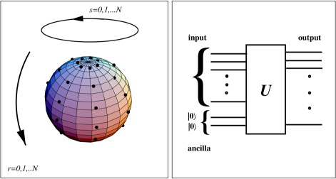
FIG. 14.: The visualization of the optimal POVM for measurement of a quantum state of the spin-1/2 from $N$ identical copies as provided by the solution in Section X A. On the right the schematic picture of an quantum network (for more information see Section X C) as a physical realization of the measuring apparatus which embodies the optimal solution from the left part of the picture.

To satisfy these completeness conditions we choose $N+1$ angles $\theta_{r}$ to be equidistantly distributed in the $\langle 0,\pi\rangle$ (obviously, there are many other choices which may suite the purpose – see discussion below Eq.(421)). Then we solve the system of linear equations for $N+1$ variables $c_{r}$. For this choice of $\theta_{r}$ the system (424) has non-negative solutions. Finally we satisfy the off-diagonal conditions by choosing $N+1$ angles $\psi_{s}={2s\pi\over N+1}$ for each $\theta_{r}$. In this case ${1\over N+1}\sum_{s=0}^{N}{\rm e}^{i\psi_{s}y}=\delta_{y,0}$ for all $y=-N/2,\dots N/2$ and the off-diagonal conditions are satisfied straightforwardly. This concludes the construction of the optimal and finite POVM for the spin-$1/2$ state estimation. In Fig. 14 we present a schematic description of the optimal POVM performed on spin-1/2, while in Fig. 15 the mean fidelity $\bar{f}$ as a function of number $N$ of measured spins (initially prepared in the same state) is presented.

FIG. 15.: The mean fidelity of the estimation of a quantum state of the spin-1/2 (lower line) and of a phase shift (upper line) based on the optimal POVM (as discussed in this Section) performed on $N$ identical copies of quantum objects under consideration. As expected, for $N$ large enough the fidelity in both cases becomes equal to unity.

B Optimal estimation of phase shifts

Consider a system of $N$ effectively two level atoms (qubits), all initially prepared in the reference state ${1\over\sqrt{2}}(|0\rangle+|1\rangle)$ by applying so called ${\pi\over 2}$ pulse to initially deexcited atoms. Then the atoms undergo the free evolution effectively described by the $U(1)$ group, i.e. the state of the single qubit evolves as ${1\over\sqrt{2}}(|0\rangle+\exp\{i\psi(t)\}|1\rangle)$. Our task is to find a measurement which provides the optimal estimation of the phase $\psi(t)$ of the $U(1)$ rotation which carries the information about the interaction parameters.

In the standard classification of representations of the $U(1)$ group the single isolated qubit is described by the direct sum of two one-dimensional representations $U=(0)\oplus(1)$. The representation $U^{N}$ transforming entire system of $N$ qubits is then equal to the direct sum of representations of the form $(0)\oplus(1)\oplus\dots(N)$. This acts in the $N+1$ dimensional space spanned by basis vectors $|m\rangle$, $m=0,1,\dots N$. In this basis matrix elements $\hat{F}_{m,n}$ of the operator $\hat{F}$ given by Eq.(414) take the form

$$\hat{F}_{m,n}=\int_{0}^{2\pi}{d\psi\over 2\pi}\ {\sqrt{(^{N}_{N-m})(^{N}_{N-n})}\over 2^{N+1}}\ {\rm e}^{i\psi(n-m)}\ (1+\cos\psi)={\sqrt{(^{N}_{N-m})(^{N}_{N-n})}\over 2^{N+2}}\left(2\delta_{m,n}+\delta_{m,n+1}+\delta_{m+1,n}\right).$$ (425)

The upper bound on the fidelity Eq. (416) is now too conservative to be of any use (greater than unity). We can, however, solve the system of Eqs. (421) which in this particular case of the commutative group reads

$$\left[\hat{F}-\hat{L}\right]|\Psi\rangle=0;\qquad|\langle m|\Psi\rangle|^{2}=1;\ \ \ \forall m.$$ (426)

The condition ${\bf Det}(\hat{F}-\hat{L})=0$ now determines the eigenvector $|\Psi\rangle$ with the zero eigenvalue as a function of Lagrange multipliers $L_{m}$. When we substitute this eigenvector into the second equation in Eq.(426) we obtain a set of equations for $L_{m}$ from which the state $|\Psi\rangle$ can be determined. The final POVM is then constructed by rotation of $|\Psi\rangle$ by $N+1$ angles $\phi_{s}$ in such a way that all off-diagonal elements of $\sum_{s}(\hat{O}_{s})_{m,n}$ become equal to zero. This is done in exactly the same way as in the example presented above. (see Section X A). The resulting POVM corresponds to the von Neumann measurement performed on the composite system of all $N$ ions characterized by the set of orthogonal projectors

$$\hat{P}_{s}=|\Psi_{s}\rangle\langle\Psi_{s}|; |\Psi_{s}\rangle={1\over\sqrt{N+1}}\sum_{q=0}^{N}{\rm e}^{i{2\pi\over N+1}sq}\ |q\rangle.$$ (427)

and the maximal mean fidelity $\bar{f}$ is given as the sum: $\bar{f}=1/2+1/2^{N+1}\sum_{i=0}^{N-1}\sqrt{(\ ^{N}_{i})(\ ^{N}_{i+1})}$. We plot this fidelity in Fig. 15 (see upper line).

Finally, we note that the Hermitian operator $\hat{\Phi}$ constructed from the optimal POVM (427)

$$\hat{\Phi}=\sum_{s-0}^{N}{2\pi\over N+1}s\hat{P}_{s},$$ (428)

with the corresponding guesses as eigenvalues is identical to the Pegg-Barnett Hermitian phase operator [83] originally introduced within completely different context.

In conclusion, we have presented a general algorithm for the optimal state estimation from finite ensembles. It provides finite POVMs which, following the Neumark theorem [84], can, at least in principle, be implemented as simple quantum computations.

C Neumark theorem and realization of generalized measurements

Applicability of many ideas presented in previous parts of this Section critically relies on the assumption that the generalized quantum measurements are in principle realizable. This is not obvious, since the typical quantum measurements, e.g. measurements which may be performed with the help of the Stern-Gerlach apparatus, a photo-detection, or a measurement of an atomic population by means of photo-ionization, etc., are all orthogonal measurements. Can we under this conditions hope to perform a controlled generalized measurement?

To answer this question we start with the following consideration: Assume a quantum object (${\cal S}$) in a state described by a density matrix $\hat{\rho}$. Instead of directly measuring it we subject this object to an interaction with another quantum object - the ancilla ${\cal A}$ (see Fig. 14). The ancilla is initially prepared in a particular (fixed) quantum state $|\alpha\rangle$. After some interaction time the composite system (${\cal S}+{\cal A}$) evolves into a nontrivial entangled quantum state $U\hat{\rho}\otimes|\alpha\rangle\langle\alpha|U^{\dagger}$. The orthogonal measurement $\{\hat{P}_{r}\}$ is then performed on the composite quantum system. In this case the conditional probability distribution $p(r|\hat{\rho})$ defined as

$$p(r|\hat{\rho})={\rm Tr_{{\cal S}+{\cal A}}}\left[\hat{P}_{r}\ U\hat{\rho}\otimes|\alpha\rangle\langle\alpha|U^{\dagger}\right]={\rm Tr_{\cal S}}\left[{\rm Tr_{\cal A}}\left[U^{\dagger}\hat{P}_{r}U\ \hat{1}\otimes|\alpha\rangle\langle\alpha|\right]\ \hat{\rho}\right]={\rm Tr_{\cal S}}\left[\hat{O}_{r}\hat{\rho}\right].$$ (429)

can be specified. It can be seen, that each projector $\hat{P}_{r}$ is associated with a new operator $\hat{O}_{r}={\rm Tr_{\cal A}}[\hat{P}_{r}\ U\hat{1}\otimes|\alpha\rangle\langle\alpha|U^{\dagger}]$. In addition, it is easy to check that the operators $\hat{O}_{r}$ together compose the nonorthogonal POVM. Therefore, the described procedure represents an orthogonal realization of a nonorthogonal POVM.

Relation between the orthogonal and the nonorthogonal POVMs is actually even more close. As showed by Neumark [84], not only any particular case of the procedure we have described realizes an nonorthogonal POVM, but also the converse is true:

Theorem (Neumark) Any POVM $\hat{O}(x)~{}dx$ defined in the Hilbert space ${\cal H}$ may arise as a restriction of an orthogonal POVM $\hat{E}(x)~{}dx$ in a larger Hilbert space $\bar{\cal H}$

$$\hat{O}(x)~{}dx=\hat{P}\hat{E}(x)\hat{P}~{}dx,$$ (430)

where $\hat{P}$ is the projection from $\bar{\cal H}$ onto ${\cal H}$.

In what follows we present a construction which proves the restricted version of this theorem. Namely, we will assume only a finite-component POVMs $\{\hat{O}_{r}\}_{r=1}^{R}$, where each component is of the form $\hat{O}_{r}=c_{r}^{2}|\Psi_{r}\rangle\langle\Psi_{r}|$. For this purpose the following construction is suitable:

Proof (special case) We are looking for a unitary transformation $U$, which satisfies the condition

$$\hat{O}_{r}={\rm Tr_{\cal A}}\left[U^{\dagger}\hat{P}_{r}U\ \hat{1}\otimes|\alpha\rangle\langle\alpha|\right];~{}~{}~{}~{}~{}~{}~{}~{}~{}~{}~{}~{}~{}~{}~{}~{}~{}\forall r=1,2,\dots R.$$ (431)

It turns out, that for the construction only $R$ of the all $d\times a$ ($a$ and $d$ is the number of dimensions of the ancilla and the measured system Hilbert spaces, respectively) dimensions of the space ${\cal H}_{{\cal S}+{\cal A}}$ are relevant. Therefore we will construct the unitary operation $U$ only on a subspace ${\cal H}^{R}\subset{\cal H}_{{\cal S}+{\cal A}}$. To have a suitable notation we also divide Hilbert space ${\cal H}^{R}$ into two subspaces ${\cal H}^{R}={\cal H}^{d}\oplus{\cal H}^{R-d}={\cal H}^{d}\oplus{\cal H}^{k}$, where the first coincides with the linear span of the vectors $|\Psi_{r}\rangle\otimes|\alpha\rangle$. By inspection, if the unitary operation $U$ is of the form

$$U=\sum_{r=1}^{R}|p_{r}\rangle\langle\psi_{r}|+\sum_{r=1}^{R}|p_{r}\rangle\langle\chi_{r}|,$$ (432)

where $|\psi_{r}\rangle\equiv c_{r}|\Psi_{r}\rangle\otimes|\alpha\rangle\in{\cal H}^{d}$ and $|\chi_{r}\rangle$ are orthogonal to all $|\psi_{s}\rangle$ (i.e. $|\chi_{r}\rangle\in H^{k}$ ), then Eq. (430) is satisfied. Therefore we need to find a proper set of vectors $|\chi_{r}\rangle$, so that $U$ is indeed a unitary transformation, i.e.

$$UU^{\dagger}=\sum_{r,s=1}^{R}\langle\psi_{r}|\psi_{s}\rangle|p_{r}\rangle\langle p_{s}|+\sum_{r,s=1}^{R}\langle\chi_{r}|\chi_{s}\rangle|p_{r}\rangle\langle p_{s}|=\hat{A}+\hat{B}=\hat{1}.$$ (433)

The operators $\hat{A}$ and $\hat{B}$ are not diagonal in the basis $|p_{r}\rangle$. However, a new basis $|\bar{p}_{r}\rangle$ can be found in which both operators $\hat{A}$ and $\hat{B}$ are diagonal. This basis is found by diagonalization of the matrix $A_{rs}=\langle\psi_{r}|\psi_{s}\rangle$ using the suitable unitary matrix $V_{rs}$ [i.e., $|\bar{p}_{r}\rangle=\sum_{s=1}^{R}V_{sr}|p_{s}\rangle$, $\bar{A}_{rs}=\sum_{i,j=1}^{R}V_{ri}^{\dagger}A_{ij}V_{js}$]. Moreover, since the following relations

$$(\hat{A}^{2})_{rs}=\sum_{i=1}^{R}A_{ri}A_{is}=(\hat{A})_{rs}, {\rm Tr}[\hat{A}]=\sum_{s=1}^{R}A_{ss}=d,$$ (434)

are satisfied (both as the consequence of the completeness condition of the original POVM) we know that the spectra of the operators $\hat{A}$ and $\hat{B}$ are: ${\rm Sp}\hat{A}=\{\overbrace{1,1,\dots 1}^{d},\overbrace{0,0,\dots 0}^{R-d}\}$; ${\rm Sp}\hat{B}=\{\overbrace{0,0,\dots 0}^{d},\overbrace{1,1,\dots 1}^{R-d}\}$. Therefore, if we use the basis $|\bar{p}_{r}\rangle$ instead of the basis $|p_{r}\rangle$ we can write the unitary transformation $U$ in the Eq. (430) in the form

$$U=\sum_{r=1}^{d}|\bar{p}_{r}\rangle\langle\bar{\psi}_{r}|+\sum_{r=d+1}^{R}|\bar{p}_{r}\rangle\langle\bar{\chi}_{r}|.$$ (435)

Because the matrices $\bar{A}_{rs}=\langle\bar{\psi}_{r}|\bar{\psi}_{s}\rangle$ and $\bar{B}_{rs}=\langle\bar{\chi}_{r}|\bar{\chi}_{s}\rangle$ are diagonal only those $|\bar{\psi}_{r}\rangle=\sum_{s=1}^{R}\langle p_{s}|\bar{p}_{r}\rangle|\psi_{s}\rangle=\sum_{s=1}^{R}V_{sr}|\psi_{s}\rangle$ and $|\bar{\chi}_{s}\rangle=\sum_{r=1}^{R}V_{rs}|\chi_{r}\rangle$ are nonzero for which $r=1,2,\dots d$ and $s=d+1,\dots R$, respectively. Moreover, this also justifies our assumption about the existence of the vectors $|\chi_{r}\rangle$ orthogonal to all $|\psi_{s}\rangle$. More exactly, as we know the vectors $|\bar{\psi}_{r}\rangle$, $r=1,2,\dots d$ we can complete them into an orthonormal basis in ${\cal H}^{R}$ by choosing the set of vectors $|\bar{\chi}_{s}\rangle$, $s=d+1,\dots R$. Because the vectors with bar are related to the vectors without bar via the unitary matrix $V_{sr}$, the vectors $|\chi_{r}\rangle$ and $|\psi_{s}\rangle$ remain mutually orthogonal. This concludes our proof.

We note, that there is a freedom in the way how we choose to complete the set of vectors $|\bar{\psi}_{r}\rangle$, $r=1,2,\dots d\$ by the vectors $|\bar{\chi}_{r}\rangle$, $r=d+1,\dots R$, so that they together form an orthonormal basis. The explicit form of the unitary operation $U$ from Eq. (430) is

$$U=\sum_{r=1}^{R}|p_{r}\rangle\langle\psi_{r}|+\sum_{r=1}^{R}|p_{r}\rangle\sum_{s=d+1}^{R}V_{rs}\langle\bar{\chi}_{s}|.$$ (436)

Therefore we conclude: If we can in the system composed of the original object and the auxiliary system perform a particular von Neumann measurement characterized by a set of orthogonal projectors $|p_{r}\rangle\langle p_{r}|$ and, in addition, we can transform this composed system by the unitary transformation $U$ [see Eq. (436)], then we can realize a general POVM measurement $\{\hat{O}_{r}\}$ (for more details see [85]).

XI INSTEAD OF CONCLUSIONS

We conclude this paper by a citation from the Jaynes’ Brandeis lectures (see p. 183 of Ref.[86]): “Conventional quantum theory has provided an answer to the problem of setting up initial state descriptions only in the limiting case where measurements of a “complete set of commuting observables” have been made, the density matrix $\hat{\rho}(0)$ then reducing to the projection operator onto a pure state $\psi(0)$ which is the appropriate simultaneous eigenstate of all measured quantities. But there is almost no experimental situation in which we really have all this information, and before we have a theory able to treat actual experimental situations, existing quantum theory must be supplemented with some principle that tells us how to translate, or encode, the results of measurements into a definite state description $\hat{\rho}(0)$. Note that the problem is not to find $\hat{\rho}(0)$ which correctly describes “true physical situation”. That is unknown, and always remains so, because of incomplete information. In order to have a usable theory we must ask the much more modest question: What $\hat{\rho}(0)$ best describes our state of knowledge about the physical situation? ”.

Appendix A

Conceptually the reconstruction scheme based on the Jaynes principle of the maximum entropy is very simple. On the other hand particular analytical calculations can be difficult and in many cases cannot be performed. In this appendix we present explicit calculations of generalized canonical density operators (GCDO) and corresponding entropies for two observation levels ${\cal O}_{G}^{(2)}$ and ${\cal O}_{H}^{(2)}$ defined in Table VI.

A. 1. Observation level ${\cal O}_{G}^{(2)}$

Let as assume the observation level ${\cal O}_{G}^{(2)}$ given by the set of observables $\{\hat{\sigma}_{z}^{(1)}\otimes\hat{\sigma}_{z}^{(2)};\hat{\sigma}_{x}^{(1)}\otimes\hat{\sigma}_{x}^{(2)};\hat{\sigma}_{x}^{(1)}\otimes\hat{\sigma}_{y}^{(2)};\hat{\sigma}_{y}^{(1)}\otimes\hat{\sigma}_{x}^{(2)};\hat{\sigma}_{y}^{(1)}\otimes\hat{\sigma}_{y}^{(2)}\}$. In this case the GCDO reads

$$\hat{\rho}_{G}={1\over{Z_{G}}}\exp\left({-\hat{E}}\right),$$

where

$$Z_{G}=\mbox{Tr}\left[{\exp\left({-\hat{E}}\right)}\right],$$

is the partition function. Here we have used the abbreviation

$$\hat{E}=\lambda_{zz}\hat{\sigma}_{z}^{(1)}\otimes\hat{\sigma}_{z}^{(2)}+\lambda_{xx}\hat{\sigma}_{x}^{(1)}\otimes\hat{\sigma}_{x}^{(2)}+\lambda_{xy}\hat{\sigma}_{x}^{(1)}\otimes\hat{\sigma}_{y}^{(2)}+\lambda_{yx}\hat{\sigma}_{y}^{(1)}\otimes\hat{\sigma}_{x}^{(2)}+\lambda_{yy}\hat{\sigma}_{y}^{(1)}\otimes\hat{\sigma}_{y}^{(2)}.$$

The corresponding entropy has the form

$$S_{G}=\ln Z_{G}+\lambda_{zz}\xi_{zz}+\lambda_{xx}\xi_{xx}+\lambda_{xy}\xi_{xy}+\lambda_{yx}\xi_{yx}+\lambda_{yy}\xi_{yy},$$

Using the algebraic properties of the operators associated with the given observation level we find the GCDO (A.1) to read

$$\hat{\rho}_{G}={1\over 4}\left[\hat{I}^{(1)}\otimes\hat{I}^{(2)}+\xi_{zz}\hat{\sigma}_{z}^{(1)}\otimes\hat{\sigma}_{z}^{(2)}+\xi_{xx}\hat{\sigma}_{x}^{(1)}\otimes\hat{\sigma}_{x}^{(2)}\right.$$

$$\left.+\xi_{xy}\hat{\sigma}_{x}^{(1)}\otimes\hat{\sigma}_{y}^{(2)}+\;\xi_{yx}\hat{\sigma}_{y}^{(1)}\otimes\hat{\sigma}_{x}^{(2)}+\xi_{yy}\hat{\sigma}_{y}^{(1)}\otimes\hat{\sigma}_{y}^{(2)}\right],$$

where we use the notation

$$\xi_{\mu\nu}\equiv\left\langle{\hat{\sigma}_{\mu}^{(1)}\otimes\hat{\sigma}_{\nu}^{(2)}}\right\rangle,\qquad(\mu,\nu=x,y,z).$$

Now we express the entropy as a function of expectation values of operators associated with the observation level ${\cal O}_{G}^{(2)}$. With the help of this entropy function we can perform reductions of ${\cal O}_{G}^{(2)}$ to the observation levels ${\cal O}_{H}^{(2)}$, ${\cal O}_{F}^{(2)}$ and ${\cal O}_{E}^{(2)}$. In order to perform this reduction we express $\lambda_{\mu\nu}$ in Eq. (A.4) as functions of the expectation values $\xi_{\mu\nu}$. To do so we utilize the relation

$$\xi_{\mu\nu}=-{{\partial\ln Z_{G}}\over{\partial\lambda_{\mu\nu}}}.$$

The partition function $Z_{G}$ can be found when we rewrite the operator $\hat{E}$ in Eq.(A.4) as a 4$\times$4 matrix:

$$\hat{E}=\left({\matrix{a&0&0&{d^{*}}\cr 0&{-a}&{b^{*}}&0\cr 0&b&{-a}&0\cr d&0&0&a\cr}}\right),$$

where we used the abbreviations

$$a=\lambda_{zz},\quad b=\lambda_{xx}+\lambda_{yy}-i(\lambda_{xy}-\lambda_{yx}),\quad d=\lambda_{xx}-\lambda_{yy}+i(\lambda_{xy}+\lambda_{yx}).$$

The powers of the operator $\hat{E}$ can be written as

$$\hat{E}^{n}=\left({\matrix{{E_{11}^{(n)}}&0&0&{E_{14}^{(n)}}\cr 0&{E_{22}^{(n)}}&{E_{23}^{(n)}}&0\cr 0&{E_{32}^{(n)}}&{E_{33}^{(n)}}&0\cr{E_{41}^{(n)}}&0&0&{E_{44}^{(n)}}\cr}}\right),$$

with the matrix elements given by the relations

$$\begin{array}[]{rcl}E_{11}^{(n)}&=&E_{44}^{(n)}={1\over 2}\left[{\left({a+\left|d\right|}\right)^{n}+\left({a-\left|d\right|}\right)^{n}}\right]\,,\\ E_{14}^{(n)}&=&{1\over 2}\left[{\left({a+\left|d\right|}\right)^{n}-\left({a-\left|d\right|}\right)^{n}}\right]{{d^{*}}\over{\left|d\right|}}\,,\\ E_{22}^{(n)}&=&E_{33}^{(n)}={1\over 2}\left[{\left({-a+\left|b\right|}\right)^{n}+\left({-a-\left|b\right|}\right)^{n}}\right]\,,\\ E_{23}^{(n)}&=&{1\over 2}\left[{\left({-a+\left|b\right|}\right)^{n}-\left({-a-\left|b\right|}\right)^{n}}\right]{{b^{*}}\over{\left|b\right|}}\,,\\ E_{32}^{(n)}&=&E_{23}^{(n)*}\,,\\ E_{41}^{(n)}&=&E_{14}^{(n)*}\,.\end{array}$$

Now we find

$$\exp\left({-\hat{E}}\right)=\left({\matrix{{e^{-a}\cosh\left|d\right|}&0&0&{-e^{-a}\sinh(\left|d\right|){{d^{*}}\over{\left|d\right|}}}\cr 0&{e^{a}\cosh\left|b\right|}&{-e^{a}\sinh(\left|b\right|){{b^{*}}\over{\left|b\right|}}}&0\cr 0&{-e^{a}\sinh(\left|b\right|){{b}\over{\left|b\right|}}}&{e^{a}\cosh\left|b\right|}&0\cr{-e^{-a}\sinh(\left|d\right|){{d}\over{\left|d\right|}}}&0&0&{e^{-a}\cosh\left|d\right|}\cr}}\right),$$

from which we obtain the expression for the partition function $Z_{G}$

$$Z_{G}=2e^{-a}\cosh\left|d\right|+2e^{a}\cosh\left|b\right|.$$

For the expectation values given by Eq.(A.7) we obtain

$$\begin{array}[]{rcl}\xi_{zz}&=&{1\over{Z_{G}}}\left[{2e^{-a}\cosh\left|d\right|-2e^{a}\cosh\left|b\right|}\right]\,;\\ \xi_{xx}&=&-{1\over{Z_{G}}}\left[{2e^{-a}\sinh(\left|d\right|){{1}\over{\left|d\right|}}\left({\lambda_{xx}-\lambda_{yy}}\right)+2e^{a}\sinh(\left|b\right|){{1}\over{\left|b\right|}}\left({\lambda_{xx}+\lambda_{yy}}\right)}\right]\,;\\ \xi_{xy}&=&-{1\over{Z_{G}}}\left[{2e^{-a}\sinh(\left|d\right|){{1}\over{\left|d\right|}}\left({\lambda_{xy}+\lambda_{yx}}\right)+2e^{a}\sinh(\left|b\right|){{1}\over{\left|b\right|}}\left({\lambda_{xy}-\lambda_{yx}}\right)}\right]\,;\\ \xi_{yx}&=&-{1\over{Z_{G}}}\left[{2e^{-a}\sinh(\left|d\right|){{1}\over{\left|d\right|}}\left({\lambda_{xy}+\lambda_{yx}}\right)-2e^{a}\sinh(\left|b\right|){{1}\over{\left|b\right|}}\left({\lambda_{xy}-\lambda_{yx}}\right)}\right]\,;\\ \xi_{yy}&=&-{1\over{Z_{G}}}\left[{-2e^{-a}\sinh(\left|d\right|){{1}\over{\left|d\right|}}\left({\lambda_{xx}-\lambda_{yy}}\right)+2e^{a}\sinh(\left|b\right|){{1}\over{\left|b\right|}}\left({\lambda_{xx}+\lambda_{yy}}\right)}\right]\,.\end{array}$$

If we introduce the abbreviations

$$B=\xi_{xx}+\xi_{yy}-i\left({\xi_{xy}-\xi_{yx}}\right)\,,\quad D=\xi_{xx}-\xi_{yy}+i\left({\xi_{xy}+\xi_{yx}}\right),$$

then with the help of Eq. (A.14) we obtain

$$B=-{4\over{Z_{G}}}e^{a}\sinh(\left|b\right|){{b}\over{\left|b\right|}}\,,\quad D=-{4\over{Z_{G}}}e^{-a}\sinh(\left|d\right|){{d}\over{\left|d\right|}}.$$

Taking into account that

$$\left|B\right|={4\over{Z_{G}}}e^{a}\sinh(\left|b\right|)\,,\quad\left|D\right|={4\over{Z_{G}}}e^{-a}\sinh(\left|d\right|),$$

we find

$${B\over{\left|B\right|}}=-{b\over{\left|b\right|}}\,,\quad{D\over{\left|D\right|}}=-{d\over{\left|d\right|}}.$$

Now we introduce four new parameters $M_{i}$

$$M_{1}=1+\xi_{zz}+\left|D\right|\,,\quad M_{2}=1+\xi_{zz}-\left|D\right|\,,\\$$

$$M_{3}=1-\xi_{zz}+\left|B\right|\,,\quad M_{4}=1-\xi_{zz}-\left|B\right|,$$

in terms of which we can express the von Neumann entropy on the given observation level. Using Eqs. (A.13), (A.14) and (A.17) we obtain

$$\begin{array}[]{rl}M_{1}={4\over{Z_{G}}}\exp\left({-a+\left|d\right|}\right)\,,&\quad M_{2}={4\over{Z_{G}}}\exp\left({-a-\left|d\right|}\right)\,,\\ M_{3}={4\over{Z_{G}}}\exp\left({a+\left|b\right|}\right)\,,&\quad M_{4}={4\over{Z_{G}}}\exp\left({a-\left|b\right|}\right).\end{array}$$

The Lagrange multipliers $\lambda_{kl}$ can be expressed as functions of the expectation values $\xi_{kl}$:

$$\exp\left(a\right)=\left({{{M_{3}M_{4}}\over{M_{1}M_{2}}}}\right)^{{1\over 4}}\,,\quad\exp\left({\left|b\right|}\right)=\left({{{M_{3}}\over{M_{4}}}}\right)^{{1\over 2}}\,,\quad\exp\left({\left|d\right|}\right)=\left({{{M_{1}}\over{M_{2}}}}\right)^{{1\over 2}}\,.$$

After inserting these expressions into Eq. (A.13) we obtain for the partition function

$$Z_{G}={4\over{\left({M_{1}M_{2}M_{3}M_{4}}\right)^{{1\over 4}}}}.$$

When we insert Eqs. (A.18), (A.21) and (A.22) into Eqs. (A.1), (A.4) and (A.12) then we find both the entropy

$$S_{G}=-\sum\limits_{i=1}^{4}{{{M_{i}}\over 4}}\ln\left({{{M_{i}}\over 4}}\right),$$

and the GCDO

$$\hat{\rho}_{G}={1\over 4}\left({\matrix{{1+\xi_{zz}}&0&0&{D^{*}}\cr 0&{1-\xi_{zz}}&{B^{*}}&0\cr 0&B&{1-\xi_{zz}}&0\cr D&{}&{}&{1+\xi_{zz}}\cr}}\right),$$

as functions of the expectation values $\xi_{kl}$. Finally, we can rewrite the reconstructed density operator (A.24) in terms of the spin operators (see Table VII).

A. 2. Observation level ${\cal O}_{H}^{(2)}$

The GCDO on the ${\cal O}_{H}^{(2)}$ can be obtained as a result of a reduction of the observation level ${\cal O}_{G}^{(2)}$. The difference between these two observation levels is that the ${\cal O}_{H}^{(2)}$ does not contain the operator $\hat{\sigma}_{z}^{(1)}\otimes\hat{\sigma}_{z}^{(2)}$, i.e., the corresponding mean value is unknown from the measurement.

According to the maximum–entropy principle, the observation level ${\cal O}_{H}^{(2)}$ can be obtained from ${\cal O}_{G}^{(2)}$ by setting the Lagrange multiplier $\lambda_{zz}$ equal to zero. With the help of the relation [see Eq.(A.7)]

$$\lambda_{zz}={{\partial S_{G}}\over{\partial\xi_{zz}}}=-{1\over 4}\ln\left({{{M_{1}M_{2}}\over{M_{3}M_{4}}}}\right)=0,$$

we obtain

$$M_{1}M_{2}=M_{3}M_{4}.$$

From this equation we find the “predicted” mean value of the operator $\hat{\sigma}_{z}^{(1)}\otimes\hat{\sigma}_{z}^{(2)}$ (i.e., the parameter $t$ in Table III)

$$\xi_{zz}={1\over 4}\left({\left|D\right|^{2}-\left|B\right|^{2}}\right)\equiv t.$$

Taking into account that the parameters $|B|$ and $|D|$ read

$$\left|B\right|^{2}=\left({\xi_{xx}+\xi_{yy}}\right)^{2}+\left({\xi_{xy}-\xi_{yx}}\right)^{2}\,,\quad\left|D\right|^{2}=\left({\xi_{xx}-\xi_{yy}}\right)^{2}+\left({\xi_{xy}+\xi_{yx}}\right)^{2}\,,$$

we can express the predicted mean value $\xi_{zz}$ as a function of the measured mean values $\xi_{xx},\,\xi_{xy},\,\xi_{yx}\,$ and $\,\xi_{yy}$:

$$\xi_{zz}=\left({\xi_{xy}\xi_{yx}-\xi_{xx}\xi_{yy}}\right)\,.$$

When we insert Eq. (A.27) into Eq. (A.19) we obtain:

$$M_{1}=N_{1}N_{2}\,,\quad M_{2}=N_{3}N_{4}\,,\quad M_{3}=N_{1}N_{3}\,,\quad M_{4}=N_{2}N_{4}\,,$$

where the parameters $N_{i}$ are defined as

$$N_{1}=1+{1\over 2}\left({\left|D\right|+\left|B\right|}\right)\,,\quad N_{2}=1+{1\over 2}\left({\left|D\right|-\left|B\right|}\right)\,,\\$$

$$N_{3}=1-{1\over 2}\left({\left|D\right|-\left|B\right|}\right)\,,\quad N_{4}=1-{1\over 2}\left({\left|D\right|+\left|B\right|}\right)\,.$$

In addition, from Eqs. (A.30) and (A.23) we obtain the expression for the von Neumann entropy of the density operator reconstructed on the observation level ${\cal O}_{H}^{(2)}$:

$$S_{H}=-\sum\limits_{i=1}^{4}{{{N_{i}}\over 2}}\ln\left({{{N_{i}}\over 2}}\right)\,.$$

Finally, from Eqs. (A.28) and (A.24) we find the expression for the GCDO on the observation level ${\cal O}_{H}^{(2)}$ (see Table VII):

$$\begin{array}[]{rcl}\hat{\rho}_{H}&=&{1\over 4}{[\hat{I}^{(1)}\otimes\hat{I}^{(2)}+\left({\xi_{xy}\xi_{yx}-\xi_{xx}\xi_{yy}}\right)\hat{\sigma}_{z}^{(1)}\otimes\hat{\sigma}_{z}^{(2)}}\\ &+&\;{\xi_{xx}\hat{\sigma}_{x}^{(1)}\otimes\hat{\sigma}_{x}^{(2)}+\xi_{xy}\hat{\sigma}_{x}^{(1)}\otimes\hat{\sigma}_{y}^{(2)}}+\;\xi_{yx}\hat{\sigma}_{y}^{(1)}\otimes\hat{\sigma}_{x}^{(2)}+\xi_{yy}\hat{\sigma}_{y}^{(1)}\otimes\hat{\sigma}_{y}^{(2)}]\,.\end{array}$$ ()

APPENDIX B: INVARIANT INTEGRATION MEASURE

In differential geometry the integration measure is a global object - the so called invariant volume form $\omega$. The condition that $d_{\Omega}$ is invariant under the action of each group element $U\in SU(n)$ is equivalent to the requirement

$$d_{{}_{\Omega}}=d_{{}_{U\Omega U^{-1}}}\ \ \Longleftrightarrow\ \ L_{V_{i}}\omega=0\qquad i=1,\dots,n^{2}-1,$$ ()

that the Lie derivative of $\omega$ with respect to the fundamental field $V_{i}$ of action of the group $SU(n)$ in the space $\Omega$ is zero. The vector fields

$$V_{i}=V^{b}_{i}(x_{1},\dots,x_{(2n-2)}){\partial\over\partial x_{b}};~{}~{}~{}b=1,2\dots(2n-2),$$ ()

are defined via the actions of one-parametric subgroups $\exp(it\hat{S}_{i})\subset SU(n),\ t\in R$ (one action for each generator $\hat{S}_{i}$). On the other hand the elements of the space $\Omega$ [see Eq.(376)] have a structure

$$\hat{\rho}(x_{1},\dots,x_{(2n-2)})={\hat{1}\over n}+f^{i}(x_{1},\dots,x_{(2n-2)})\hat{S}_{i},$$ ()

where $\hat{S}_{i}$ are $n^{2}-1$ linearly independent, zero-trace, Hermitian, $n\times n$ matrixes, i.e. they are generators of the $SU(n)$ group. Due to this we can express the vector fields $V_{i}$

$$V^{b}_{i}{\partial\over\partial x_{b}}\hat{\rho}={\partial\over\partial t}\left.\left[\exp(it\hat{S}_{i})\hat{\rho}\exp(-it\hat{S}_{i})\right]\right|_{t=0},$$ ()

as the solutions of the following equation:

$$V^{b}_{i}{\partial\over\partial x_{b}}f^{k}=ic^{k}_{ij}f^{j}.$$ ()

The complex numbers $c^{k}_{ij}$ are the coefficients in commutation relations $[\hat{S}_{i},\hat{S}_{j}]=c^{k}_{ij}\hat{S}_{k}$. We note, that Eq. (() ‣ APPENDIX B: INVARIANT INTEGRATION MEASURE) represents for each fixed index $i$ an overdetermined system of $n^{2}-1$ linear equations for $2n-2$ unknown functions $V^{b}_{i}$ (the fact that this system is consistent confirms the correctness of our parameterization of the state space $\Omega$). Finally, we present an explicit coordinate form of Eq.(() ‣ APPENDIX B: INVARIANT INTEGRATION MEASURE), which determines the invariant volume form $\omega=m(x_{1},\dots,x_{(2n-2)})\land dx_{1}\land\dots\land dx_{(2n-2)}$ as the solution of a system of partial differential equations:

$${\partial\over\partial x_{b}}(mV_{i}^{b})=0.$$ ()

Here we note, that $m\vec{V}_{i}$ in Eq.(() ‣ APPENDIX B: INVARIANT INTEGRATION MEASURE) has the meaning of a “flow” of the density of states generated by unitary transformations associated with the $i$-th generator. From the physical point of view Eq.(() ‣ APPENDIX B: INVARIANT INTEGRATION MEASURE) means that the divergence of this flow is zero, i.e. the number of states in each (confined) volume element is constant.

As an illustration of the above discussion we firstly evaluate the invariant measure for the state space of a single spin-1/2. Using the definition (() ‣ APPENDIX B: INVARIANT INTEGRATION MEASURE) we find the fundamental field of action $V_{i}$ ($i=1,2,3$) for the three generators of the $SU(2)$ group:

$$V_{1}=\cos(\phi)\cot(\theta)\partial_{\phi}+\sin(\phi)\partial_{\theta};\ \ \ \ V_{2}=\sin(\phi)\cot(\theta)\partial_{\phi}-\cos(\phi)\partial_{\theta};\ \ \ \ V_{3}=-\partial_{\phi}.$$ ()

We substitute these generators into Eq.(() ‣ APPENDIX B: INVARIANT INTEGRATION MEASURE) and after some algebra we obtain the system of differential equations:

$${\partial\over\partial\phi}m=0\qquad{\partial\over\partial\theta}m=m\cot(\theta),$$ ()

which can be easily solved,

$$m(\theta,\phi)=const\ \sin(\theta).$$ ()

The multiplicative factor is given by the normalization condition. This is the route to derive the integration measure of the Poincaré sphere. Analogously we evaluate the invariant integration measure for a state space of two spins-1/2. The calculations are technically more involved, but the result is simple see Eq. (381).

Appendix C: Bayesian inference on ${\cal O}_{B}^{(2)}$ in the limit of infinite number of measurements

On the given observation level we can express the estimated density operator in the limit of infinite number of measurements as

$$\hat{\rho}=\frac{1}{\cal N}\int_{0}^{2\pi}\!\!d\psi\!\!\int_{-1}^{1}\!\!x^{2}dx\!\!\int_{-1}^{1}\!\!dy\!\!\int_{-1}^{1}\!\!dz\delta\left(\langle\hat{\sigma}_{z}^{{}_{(1)}}\rangle-xy)\delta(\langle\hat{\sigma}_{z}^{{}_{(1)}}\hat{\sigma}_{z}^{{}_{(2)}}\rangle-yz+\left[(1-x^{2})(1-y^{2})(1-z^{2})\right]^{1/2}\cos\psi\right)$$ (439)

$$\times\left\{\hat{1}\otimes\hat{1}+xy\hat{\sigma}_{z}\otimes\hat{1}+xz\hat{1}\otimes\hat{\sigma}_{z}+\left[yz-\left((1-x^{2})(1-y^{2})(1-z^{2})\right)^{1/2}\cos\psi\right]\hat{\sigma}_{z}\otimes\hat{\sigma}_{z}\right\}.$$ ()

When we integrate Eq.(() ‣ Appendix C: Bayesian inference on ${\cal O}_{B}^{(2)}$ in the limit of infinite number of measurements) over the variable $y$ and we obtain

$$\hat{\rho}=\frac{1}{\cal N}\int_{0}^{2\pi}\,d\psi\int_{{\cal L}^{\prime}}{x^{2}\over|x|}dx\!\!\int_{-1}^{1}\,dz\delta\left(\langle\hat{\sigma}_{z}^{{}_{(1)}}\hat{\sigma}_{z}^{{}_{(2)}}\rangle-\langle\hat{\sigma}_{z}^{{}_{(1)}}\rangle{z\over x}+\left[(1-x^{2})(1-z^{2})\left(1-{\langle\hat{\sigma}_{z}^{{}_{(1)}}\rangle^{2}\over x^{2}}\right)\right]^{1/2}\cos\psi\right)$$ (440)

$$\times\left\{\hat{1}\otimes\hat{1}+\langle\hat{\sigma}_{z}^{{}_{(1)}}\rangle\hat{\sigma}_{z}\otimes\hat{1}+xz\hat{1}\otimes\hat{\sigma}_{z}+\left[\langle\hat{\sigma}_{z}^{{}_{(1)}}\rangle{z\over x}\right.\right.$$ (441)

$$\left.\left.-\left((1-x^{2})(1-z^{2})\left(1-{\langle\hat{\sigma}_{z}^{{}_{(1)}}\rangle^{2}\over x^{2}}\right)\right)^{1/2}\cos\psi)\right]\hat{\sigma}_{z}\otimes\hat{\sigma}_{z}\right\},$$ ()

where the integration boundaries are defined as

$${\cal L}^{\prime\prime}:=\{-1,1\}~{}~{}~{}{\mbox{\rm and}}~{}~{}~{}|x|\geq|\langle\hat{\sigma}_{z}^{{}_{(1)}}\rangle|.$$ ()

Now we will integrate Eq.(() ‣ Appendix C: Bayesian inference on ${\cal O}_{B}^{(2)}$ in the limit of infinite number of measurements) over the variable $\psi$. There are two values $\psi_{0}^{(j)}$ ($j=1,2$) of $\psi$, such that

$$\cos\psi_{0}={\langle\hat{\sigma}_{z}^{{}_{(1)}}\hat{\sigma}_{z}^{{}_{(2)}}\rangle-\langle\hat{\sigma}_{z}^{{}_{(1)}}\rangle{z/x}\over\left[(1-x^{2})(1-z^{2})(1-(\langle\hat{\sigma}_{z}^{{}_{(1)}}\rangle/x)^{2})\right]^{1/2}},$$ ()

providing that inequality

$$1\geq\left|{\langle\hat{\sigma}_{z}^{{}_{(1)}}\hat{\sigma}_{z}^{{}_{(2)}}\rangle-\langle\hat{\sigma}_{z}^{{}_{(1)}}\rangle z/x}\over{\left[(1-x^{2})(1-z^{2})(1-(\langle\hat{\sigma}_{z}^{{}_{(1)}}\rangle/x)^{2})\right]^{1/2}}\right|.$$ ()

holds. The last relation can be rewritten as the condition $a+bz+cz^{2}\geq 0$, where the explicit forms of the coefficients $a,b$, and $c$ are:

$$a=1-\langle\hat{\sigma}_{z}^{{}_{(1)}}\rangle^{2}/x^{2}+\langle\hat{\sigma}_{z}^{{}_{(1)}}\rangle^{2}-\langle\hat{\sigma}_{z}^{{}_{(1)}}\hat{\sigma}_{z}^{{}_{(2)}}\rangle^{2}-x^{2};$$ (442)

$$b=2\langle\hat{\sigma}_{z}^{{}_{(1)}}\rangle\langle\hat{\sigma}_{z}^{{}_{(1)}}\hat{\sigma}_{z}^{{}_{(2)}}\rangle/x;\qquad c=x^{2}-\langle\hat{\sigma}_{z}^{{}_{(1)}}\rangle^{2}-1.$$ ()

The coefficient $c$ is always negative, which means that we have a new condition for the parameter $z$, that is $z\in\langle z_{1},z_{2}\rangle$, where $z_{1}$ and $z_{2}$ are two roots of the quadratic equation $a+bz+cz^{2}=0$. However, these roots exist only providing the discriminant $b^{2}-4ac\geq 0$ is nonnegative. Taking into account Eq.(() ‣ Appendix C: Bayesian inference on ${\cal O}_{B}^{(2)}$ in the limit of infinite number of measurements) we see that the last relation is a cubic equation with respect to the variable $x^{2}$, which imposes a new condition on the integration parameter $x$. That is, the interval ${\cal L}^{\prime\prime}$ through which the integration over $x$ in Eq.(() ‣ Appendix C: Bayesian inference on ${\cal O}_{B}^{(2)}$ in the limit of infinite number of measurements) is performed is defined as

$${\cal L}^{\prime\prime}:=\left\{\begin{tabular}[]{ll}$\left\{|\langle\hat{\sigma}_{z}^{{}_{(1)}}\rangle|,1\right\}$&$\mbox{\rm~{}~{}for~{}~{}}|\langle\hat{\sigma}_{z}^{{}_{(1)}}\hat{\sigma}_{z}^{{}_{(2)}}\rangle|\leq|\langle\hat{\sigma}_{z}^{{}_{(1)}}\rangle|;$\\ $\left\{|\langle\hat{\sigma}_{z}^{{}_{(1)}}\rangle|,\sqrt{1+\langle\hat{\sigma}_{z}^{{}_{(1)}}\rangle^{2}-\langle\hat{\sigma}_{z}^{{}_{(1)}}\hat{\sigma}_{z}^{{}_{(2)}}\rangle^{2}}\right\}$&$\mbox{\rm~{}~{}~{}for~{}~{}~{}}|\langle\hat{\sigma}_{z}^{{}_{(1)}}\hat{\sigma}_{z}^{{}_{(2)}}\rangle|\geq|\langle\hat{\sigma}_{z}^{{}_{(1)}}\rangle|.$\end{tabular}\right.$$ ()

Taking into account all conditions imposed on parameters of integration we can rewrite Eq.(() ‣ Appendix C: Bayesian inference on ${\cal O}_{B}^{(2)}$ in the limit of infinite number of measurements) as

$$\hat{\rho}=\frac{1}{\cal N}\int_{{\cal L}^{\prime\prime}}\,{x^{2}\over|x|}dx\!\!\int_{z_{1}}^{z_{2}}{dz\over\sqrt{a+bz+cz^{2}}}(\hat{1}\otimes\hat{1}+\langle\hat{\sigma}_{z}^{{}_{(1)}}\rangle\hat{\sigma}_{z}\otimes\hat{1}+xz\hat{1}\otimes\hat{\sigma}_{z}+\langle\hat{\sigma}_{z}^{{}_{(1)}}\hat{\sigma}_{z}^{{}_{(2)}}\rangle\hat{\sigma}_{z}\otimes\hat{\sigma}_{z}).$$ ()

Using standard formulas [see, for example, [74], Eq.(2.261) and Eq.(2.264)] the integration over parameter $z$ in Eq.(() ‣ Appendix C: Bayesian inference on ${\cal O}_{B}^{(2)}$ in the limit of infinite number of measurements) can now be performed and we obtain

$$\hat{\rho}=\frac{1}{\cal N}\int_{{\cal L}^{\prime\prime}}\,dx{x^{2}\over|x|}{1\over(1+\langle\hat{\sigma}_{z}^{{}_{(1)}}\rangle^{2}-x^{2})^{1\over 2}}(\hat{1}\otimes\hat{1}+\langle\hat{\sigma}_{z}^{{}_{(1)}}\rangle\hat{\sigma}_{z}\otimes\hat{1}+\langle\hat{\sigma}_{z}^{{}_{(1)}}\hat{\sigma}_{z}^{{}_{(2)}}\rangle\hat{\sigma}_{z}\otimes\hat{\sigma}_{z})$$ (445)

$$+\int_{{\cal L}^{\prime\prime}}\,dx{x^{2}\over|x|}{\langle\hat{\sigma}_{z}^{{}_{(1)}}\rangle\langle\hat{\sigma}_{z}^{{}_{(1)}}\hat{\sigma}_{z}^{{}_{(2)}}\rangle\over(1+\langle\hat{\sigma}_{z}^{{}_{(1)}}\rangle^{2}-x^{2})^{3\over 2}}(\hat{1}\otimes\hat{\sigma}_{z}).$$ ()

After performing integration over $x$ in Eq.(() ‣ Appendix C: Bayesian inference on ${\cal O}_{B}^{(2)}$ in the limit of infinite number of measurements) we obtain final the expression (391) for the a posteriori estimation of the density operator on the given observation level.

REFERENCES

- [1] A. Peres: Quantum Theory: Concepts and Methods (Kluwer Academic Publishers, Dordrecht, 1993).
- [2] R. Omnès: The Interpretation of Quantum Mechanics (Princeton University Press, Princeton, NJ, 1994).
- [3] L.E. Ballentine: Quantum Mechanics (Prentice Hall, Englewood Cliffs, New Jersey, 1990).
-
[4]
W. Band and J.L. Park,
Am. J. Phys. 47, 188 (1979);
Found. Phys. 1, 133 (1970);
Found. Phys. 1, 339 (1971);
J.L. Park and W. Band, Found. Phys. 1, 211 (1971). - [5] R.G.Newton and Bing-Lin Young, Ann. Phys. (N.Y.) 49, 393 (1968).
-
[6]
J. von Neumann: Mathematical Foundations of Quantum Mechanics
(Princeton University Press, Princeton, 1955) see also
J.A. Wheeler and W.H. Zurek: Quantum Theory and Measurement (Princeton University Press, Princeton, 1983). -
[7]
W. Pauli:
General Principles of Quantum Mechanics
(Springer Verlag, Berlin, 1980); see also
B. d’ Espagnat: Conceptual Foundations of Quantum Mechanics, 2nd ed. (W.A.Benjamin, Reading, 1976). -
[8]
W. Gale, E. Guth, and G.T. Trammel,
Phys. Rev. 165, 1434 (1968); see also
A. Orlowski and H. Paul, Phys. Rev. 50, R921 (1994). -
[9]
K.Vogel and H.Risken,
Phys. Rev. A 40, 2847 (1989); see also
J.Bertrand and P.Bertrand, Found. Phys. 17, 397 (1987);
M.Freyberger, K.Vogel, and W.P.Schleich, Phys. Lett. A 176, 41 (1993);
G.S.Agarwal and S.Chaturvedi, Phys. Rev. A 49, R665 (1994);
W.Vogel and D.-G.Welsch, Acta Phys. Slov. 45, 313 (1995);
U. Leonhardt and H. Paul, Phys. Lett. A 193, 117 (1994);
U. Leonhardt and H. Paul, J. Mod. Opt. 41, 1427 (1994);
H. Kühn, D.-G. Welsch, and W.Vogel, J. Mod. Opt. 41, 1607 (1994);
U.Leonhardt, Phys. Rev. A 48, 3265 (1993);
U.Leonhardt and H.Paul, Phys. Rev. A 48, 4598 (1993);
H.Paul, U.Leonhardt and G.M.D’Ariano, Acta Phys. Slov. 45, 261 (1995). -
[10]
D.T. Smithey, M. Beck, M.G. Raymer and A. Faridani,
Phys. Rev. Lett.70, 1244 (1993);
D.T. Smithey, M. Beck, J. Cooper and M.G. Raymer, Phys. Scr. T 48, 35 (1993);
M. Beck, M.G. Raymer, I.A. Walmsley, and V. Wong, Opt. Lett. 18, 2041 (1993).
M. Beck, D.T. Smithey, and M.G. Raymer, Phys. Rev. A 48, R890 (1993);
M.G. Raymer, M. Beck, and D.F. Mc Alister, Phys. Rev. Lett. 72, 1137 (1994);
M.G. Raymer, D.T. Smithey, M. Beck, and J. Cooper, Acta Phys. Pol. 86, 71 (1994). - [11] M. Munroe, D. Boggavarapu, M.E. ANderson, and M.G. Raymer, Phys. Rev. A 52, R924 (1995).
- [12] U.Leonhardt: Measuring teh quantum state of light (Cambridge University Press, Cambridge, 1997).
- [13] D.-G. Welsch, W.Vogel, and T. Opatrný: Homodyne detection and quantum state reconstruction, in Progress in Optics, ed. by E. Wolf (North Holland, Amsterdam, to appear).
- [14] G.M. D’Ariano, C. Machiavelo, and M.G.A. Paris, Phys. Rev. A 50, 4298 (1994);
- [15] U. Leonhardt, M. Munroe, T. Kiss, T. Richter, and M.G. Raymer, Opt. Commun. 127, 144 (1996).
- [16] A. Royer, Found. Phys. 19, 3 (1989), Phys. Rev. Lett. 55, 2745 (1985)
- [17] U. Janicke and M. Wilkens, J. Mod. Opt. 42, 2183 (1995).
-
[18]
Ch. Kurtsiefer, T. Pfau, and J. Mlynek:
Measurement of the Wigner function of matter wave packet,
in Technical Digest of the European Quantum Electronic Conference,
(Hamburg, Germany, 1996), p.132;
S. Schiller, G. Breitenbach, S.F. Pereira, T. Müller, and J. Mlynek, Phys. Rev. Lett. 77, 2933 (1996);
Ch. Kurtsiefer, T. Pfau, and J. Mlynek, Nature 386, 150 (1997). -
[19]
S. Wallentowitz and W. Vogel, Phys. Rev. Lett. 75, 2932 (1995);
J.F. Poyatos, R. Walser, J.I. Cirac, P. Zoller, and R. Blatt, Phys. Rev. A 53, R1966 (1996);
C.D’Helon and G.J. Milburn, Phys. Rev. A 53, R25 (1996). -
[20]
D. Leibfried, D.M. Meekhof, B.E. King, C. Monroe, W.M. Itano, and
D.J. Wineland,
Phys. Rev. Lett. 77, 4281 (1996);
D. Leibfried, D.M. Meekhof, C. Monroe, B.E. King, W.M. Itano, and D.J. Wineland, J. Mod. Opt. 44, 2485 (1997);
D.Wineland, C.Monroe, D.M.Meekhof, B.E.King, D.Liebfried, W.M.Itano, J.C.Bergquist, D.Berkeland, J.J.Bollinger, and J.Miller, Proc. Roy. Soc. A 454, 411 (1998). - [21] T.J. Dunn, I.A. Walmsley, and S. Mukamel, Phys. Rev. Lett. 74, 884 (1995).
-
[22]
U.Leonhardt, Phys.Rev.Lett. 74, 4101 (1995);
Phys. Rev. A 53, 2998 (1996); see also
W.K.Wootters, Found. Phys. 16, 391 (1986).
W.K.Wootters, Ann. Phys. (N.Y.) 175, 1 (1987);
D.Galetti and A.F.R. De Toledo Piza, Physica A 149, 267 (1988). -
[23]
A. Barenco and A.K.Ekert,
Acta Phys. Slovaca 45, 205 (1995);
A. Barenco, Contemp. Phys. 37, 359 (1996), and references therein.
A. Steane: Quantum Computing [Los Alamos e-print archive quant-ph/9708022];
D. DiVincenzo, Proc. Roy. Soc. 454, 261 (1998). -
[24]
R. Walser, J.I. Cirac, and P. Zoller,
Phys. Rev. Lett. 77, 2658 (1996); see also
A.S. Parkins, P. Marte, P. Zoller, O. Carnal, and H.J. Kimble, Phys. Rev. A 51, 1578 (1995);
A.S. Parkins, P. Marte, P. Zoller, and H.J. Kimble, Phys. Rev. Lett. 71, 3095 (1993). -
[25]
K. Husimi,
Proc. Phys. Math. Soc. Jpn. 22, 264 (1940);
Y. Kano, J. Math. Phys. 6, 1913 (1965). -
[26]
E. Arthurs and J.L. Kelly, Jr.,
Bell. Syst. Tech. J. 44, 725 (1965);
W.K. Wootters and W.H. Zurek, Phys. Rev. D 19, 473 (1979);
Y.Lai and H.A.Haus, Quantum Opt. 1, 99 (1989);
D.Lalović, D.M.Davidović, and N.Bijedić, Phys. Rev. A 46, 1206 (1992);
D.M.Davidović and D.Lalović, J. Phys. A 26, 5099 (1993);
S.Chaturvedi, G.S.Agarwal, and V.Srinivasan, J. Phys.A 27, L39 (1994);
M.G.Raymer, Am. J. Phys. 62, 986 (1994);
V. Bužek, C.H. Keitel, and P.L. Knight, Phys. Rev. A 51, 2575 (1995). - [27] S.Stenholm, Ann. Phys. (N.Y.) 218, 233 (1992).
- [28] U. Leonhardt and H. Paul, Quant. Electron. 19, 89 (1995).
-
[29]
K. Wódkiewicz
Phys. Rev. Lett. 52, 1064 (1984);
K. Wódkiewicz Phys. Lett. A 115, 304 (1986);
K. Wódkiewicz Phys. Lett. A 129, 1 (1988). - [30] C.W. Helstrom: Quantum Detection and Estimation Theory (Academic Press, New York, 1976).
- [31] A.S. Holevo: Probabilistic and Statistical Aspects of Quantum Theory (North-Holland, Amsterdam, 1982).
-
[32]
N.G. Walker and J.E. Carroll, Opt. Quant. Electron. 18, 335 (1986);
N.G. Walker, J. Mod. Opt. 34, 15 (1987). - [33] J.W. Noh, A. Fougéres, and L. Mandel, Phys. Rev. Lett. 67, 1426 (1991); Phys. Rev. A 45, 424 (1992).
-
[34]
Y. Lai and H.A. Haus, Quant. Opt. 1, 99 (1989);
Z. Hradil, Quant. Opt. 4, 93 (1992). - [35] A. Wünsche, and V. Bužek, J. Quant. Semiclass. Optics 9, 631 (1997).
-
[36]
T. Opatrný, V. Bužek, J. Bajer, and G. Drobný,
Phys. Rev. A 52, 2419 (1995);
T. Opatrný, D.-G. Welsch, and V. Bužek, Phys. Rev. A 53, 3822 (1996). - [37] E.T. Jaynes, Phys. Rev. 108, 171 (1957); ibid. 108, 620 (1957) 620; Am. J. Phys. 31, 66 (1963).
- [38] E. Fick and G. Sauermann: The Quantum Statistics of Dynamic Processes (Springer Verlag, Berlin, 1990).
- [39] J.N.Kapur and H.K.Kesavan: Entropic Optimization Principles with Applications (Academic Press, New York, 1992).
-
[40]
A. Katz:
Principles of Statistical Mechanics,
(W.H. Freeman and Company, San Francisco, 1967);
A. Hobson, Concepts in Statistical Mechanics, (Gordon Breach Science Publishers, New York, 1971). -
[41]
V. Bužek, G. Adam, and G. Drobný, Ann. Phys. (N.Y.) 245,
37 (1996);
V. Bužek, G. Adam, and G. Drobný, Phys. Rev. A 54, 801 (1996). - [42] K.R.W. Jones, Ann. Phys. (N.Y.) 207, 140 (1991); Phys. Rev. A 50, 3682 (1994).
-
[43]
R. Derka, V. Bužek, and G. Adam, Acta Phys. Slov.
46, 355 (1996);
R. Derka, V. Bužek, G. Adam, and P.L. Knight, J. of Fine Mechanics & Optics, No. 11/12, p. 341 (1996);
V. Bužek, R. Derka, G. Adam, and P.L. Knight, Annals of Physics (N.Y.), to appear (1998). - [44] S. Massar and S. Popescu, Phys. Rev. Lett. 74, 1259 (1995)
- [45] R. Derka, V. Bu]vzek, and A.K. Ekert, Phys. Rev. Lett 80, 1571 (1998).
- [46] A. Wehrl, Rev. Mod. Phys. 50, 221 (1978).
- [47] B. Robertson, Phys. Rev., 144, 151 (1966); ibid. 166, 175 (1967); ibid. 166, 206 (1968).
-
[48]
G. Adam and J. Seke,
Phys. Rev. A, 23, 3118 (1980);
H. Schwegler, Z. Naturforschung, 20a, 1543 (1965);
J. Seke, Phys. Rev. A, 21, 2156 (1980);
J. Seke, G. Adam, and O. Hittmair, Sitzungsber. d. Österr. Akad. d. Wiss., math.–naturw. Kl., Wien, 194, 169 (1985); Acta Physica Austriaca, 56, 225 (1985). -
[49]
R.J.Glauber,
Phys. Rev. Lett. 10, 84 (1963);
E.C.G.Sudarshan, Phys. Rev. Lett. 10, 277 (1963). -
[50]
E.P.Wigner, Phys. Rev. 40, 749 (1932); see also
E.P. Wigner, in Perspectives in Quantum Theory, eds. W.Yourgrau and A. van der Merwe (Dover, New York, 1979), p.25;
H.Weyl: “The Theory of Groups and Quantum Mechanics” (Dover, New York, 1950);
S.Stenholm, Eur. J. Phys. 1, 244 (1980);
V.I.Tatarskij, Sov. Phys. Usp. 26, 311 (1983);
M.Hillery, R.F.O’Connell, M.O.Scully, and E.P.Wigner, Phys. Rep. 106, 121 (1984). - [51] K.E.Cahill and R.J.Glauber, Phys.Rev., 177, 1857 (1969); 177, 1882 (1969).
- [52] A.K.Ekert and P.L.Knight, Phys. Rev. A 43, 3934 (1991).
- [53] H. Kühn, D.-G. Welsch, and W. Vogel, J. Mod. Opt. 41, 1607 (1994).
-
[54]
R.Schack and A.Schenzle,
Phys. Rev. A 41, 3847 (1990);
J.Peřina, J.Křepelka, R.Horák, Z.Hradil, and J.Bajer, Czech. J. Phys. B 37, 1161 (1987). - [55] U. Leonhardt, H. Paul, and G.M. D’Ariano, Phys. Rev. A 52, 4899 (1995);
-
[56]
Th. Richter, Phys. Lett. A 211, 327 (1996);
Th. Richter, Phys. Rev. A 53, 1197 (1996); - [57] G.M. D’Ariano, U. Leonhardt, and H. Paul, Phys. Rev. A 52, R1801 (1995);
-
[58]
R.Loudon and P.L.Knight;
J. Mod. Opt. 34, 709 (1987);
K.Zaheer and M.S.Zubairy, in: Advances in Atomic, Molecular, and Optical Physics, Vol.28, eds. D.Bates and B.Bederson (Academic Press, New York, 1991), p.143;
S.M. Barnett and P.M. Radmore: Methods in Theoretical Quantum Optics (Clarendon Press, Oxford, 1997). -
[59]
V.Bužek, A.Vidiella-Barranco, and P.L.Knight,
Phys.Rev. A 45, 6570 (1992);
V.Bužek and P.L.Knight: Quantum interference, superposition states of light and nonclassical effects, in Progress in Optics, Vol. 34, ed. E. Wolf (North Holland, Amsterdam, 1995), p.1. - [60] M.Brune, S.Haroche, J.M.Raimond, L.Davidovich, and N.Zagury, Phys. Rev. A 45, 5193 (1992).
-
[61]
V.V.Dodonov, I.A.Malkin, and V.I.Manko,
Nuovo Cimento 24B, 46 (1974);
Physica 72, 597 (1974);
I.A.Malkin and V.I.Manko, Dynamical Symetries and Coherent States of Quantum Systems, (Nauka, Moscow, 1979). - [62] W.H.Louisell, Quantum Statistical Properties of Radiation, (John Wiley & Sons, New York, 1973).
- [63] C.W.Gardiner, Quantum Noise, (Springer-Verlag, Berlin, 1991)
-
[64]
V.V.Dodonov, E.Kurmyshev, and V.I.Manko,
Phys. Lett. A 76, 150 (1980);
R.L.Hudson, Rep. Math. Phys. 6, 249 (1974);
B.L.Schumaker, Phys. Rep. 135, 317 (1986). -
[65]
R.A.Fischer, M.M.Nieto, and V.D.Sandberg,
Phys. Rev. D 29, 1107 (1984);
S.L.Braunstein and R.I.Mc Lachlan, Phys. Rev. A 35, 1659 (1987);
M.Hillery, Phys. Rev. A 42, 498 (1990). - [66] C.E.Shannon, Bell. Sys. Techn. J. 27, 379 (1948); ibid. 27, 623 (1948).
-
[67]
U. Leonhardt and M. Munroe, Phys. Rev. A 54, 3682 (1996); see
also
A. Wünsche, Phys. Rev. A 54, 5291 (1996). -
[68]
T. Opatrný and D.-G. Welsch, Phys. Rev. A 55, 1462 (1997);
S.M. Tan, J. Mod. Opt. 44, 2233 (1997) and references therein. - [69] W.Vogel and W.P.Schleich, Phys. Rev. A 44, 7642 (1991).
- [70] V.Bužek, G.Drobný, G.Adam, R.Derka, and P.L.Knight, J. Mod. Opt. 44 2607 (1997).
-
[71]
D.M. Greenberger, M.H. Horne and A. Zeilinger,
Bell’s Theorem, Quantum Theory, and Conceptions of the Universe,
ed.M.Kafatos (Kluwer, Dortrecht, 1989);
D.M. Greenberger, M.H. Horne and A. Zeilinger, Physics Today, No.8 (August), 22 (1993). -
[72]
H. Jeffreys: Theory of Probability
(Oxford Univ. Press., Oxford, 1960); see also
R.vonMises, Mathematical Theory of Probability and Statistics (Academy Press, New York, 1964). -
[73]
Z. Hradil, Phys. Rev. A 55, R1561 (1997); see also
D. Mogiltsev, Z. Hradil, and J. Peřina, J. Mod. Opt. 44, 2261 (1997). - [74] I.S. Gradstein and I.M. Ryzhik: Table of Integrals, Series, and Products (Academic Press, New York, 1980).
- [75] A. Peres Phys. Rev. Lett. 77, 1413 (1996); M. Horodecki, P. Horodecki, and R. Horodecki, Phys. Lett. A 223, 1 (1996); Phys. Rev. Lett. 78, 574 (1997).
- [76] A. Uhlmann, Rep. Math. Phys. 9, 273 (1976); ibid 24, 229 (1986).
- [77] A.K. Ekert and P.L. Knight, Am. J. Phys. 63, 415 (1995).
-
[78]
S.L. Braunstein and C.M. Caves, Phys. Rev. Lett. 72, 3439 (1994);
see also
S.L. Braunstein and C.M. Caves, Annals of the New York Acad. Sci. 755, 798 (1995);
S.L. Braunstein, Phys. Lett. A 219, 169 (1996). -
[79]
D. Bures, trans. Am. Math. Soc. 135, 199 (1969);
M. Hübner, Phys. Lett. A 163, 239 (1992); ibid 179, 226 (1993);
J. Twamley, J. Phys. A, 29, 3723 (1996). - [80] P.B. Slater, Physica A, 214, 584 (1995).
- [81] A.O. Barut and R. Raczka, Theory of Group Representations and applications (World Scientific, Singapore, 1986)
- [82] R.N. Zare, Angular Momentum (Wiley, New York, 1988)
- [83] D.T. Pegg and S.M. Barnett, Europhys. Lett. 6, 483 (1988)
- [84] M.A. Neumark, C.R. Acad. Sci. USSR 41, 359 (1943)
- [85] R.Derka and V.Bužek, Optimal estimation of quantum states from finite ensembles: From pure theory to hypothetic experiments, unpublished.
- [86] E.T. Jaynes, Information theory and statistical mechanics, in 1962 Brandeis Lectures, Vol 3, ed. K.W. Ford (Benjamin, Inc. New York, 1963), p.181.