Quantum Oracle Interrogation:
Getting All Information for Almost Half the Price

Abstract

Consider a quantum computer in combination with a binary oracle of domain size $N$. It is shown how $N/2+\sqrt{N}$ calls to the oracle are sufficient to guess the whole content of the oracle (being an $N$ bit string) with probability greater than 95%. This contrasts the power of classical computers which would require $N$ calls to achieve the same task. From this result it follows that any function with the $N$ bits of the oracle as input can be calculated using $N/2+\sqrt{N}$ queries if we allow a small probability of error. It is also shown that this error probability can be made arbitrary small by using $N/2+O(\sqrt{N})$ oracle queries.

In the second part of the article ‘approximate interrogation’ is considered. This is when only a certain fraction of the $N$ oracle bits are requested. Also for this scenario does the quantum algorithm outperform the classical protocols. An example is given where a quantum procedure with $N/10$ queries returns a string of which 80% of the bits are correct. Any classical protocol would need $6N/10$ queries to establish such a correctness ratio.

1 Introduction

Recent research [1, 6, 9] in quantum computation complexity has revealed several lower bounds on the capability of quantum computers to outperform classical computers in the black-box setting. These results were proven by investigating the required amount of queries to a black-box or oracle (with a domain size $N$) in order to decide some general property of this function. For example, if we want to know the parity of the $N$ black-box values with bounded error then it is still necessary for a quantum computer to call the black-box $N/2$ times[1, 6]. It has also been shown that for the exact calculation of certain functions (the bitwise or for example) all $N$ calls are required[1].

This paper on the other hand, presents an upper bound on the number of black-box queries that is necessary to compute any function over the $N$ bits if we allow a small probability of error. More specifically, it will be shown that for every unknown oracle there is a potential speed-up of almost a factor of two if we want to know everything there is to know about the oracle function. By this the following is meant. If the domain of the oracle has size $N$, a classical computer will have to apply $N$ calls in order to know all $N$ bits describing the oracle. Here, it will be proven that a quantum computer can perform the same task with high probability using only $N/2+\sqrt{N}$ oracle calls. From this result it follows immediately that any (not necessarily binary) function $F$ on the domain ${\{0,1\}}^{N}$ can be calculated with a small two-sided error using only $N/2+\sqrt{N}$ calls.

The factor–of–two gain can be increased by going to approximating interrogation procedures. If we do not longer require to know all of the $N$ bits but are instead already satisfied with a certain percentage of correct bits, then the difference between classical and quantum computation becomes bigger than for the above ‘exact interrogation’ case. An example of this is when we want to guess the string such that we can expect 80% of the bits to be correct. A quantum computer can do this with one-sixth of the queries that a classical computer requires ($N/10$ versus $3N/5$ calls). This also illustrates that the procedure described here is not a ‘superdense coding–in–disguise’ which would only allow a reduction by a factor of two[2].

2 Preliminaries

The setting for this article is as follows. We try to investigate the potential differences between a quantum and a classical computer when both cases are confronted with an oracle $\omega$. The only thing known in advance about this $\omega$ is that it is a binary-valued function with a domain of size $N$. The oracle can therefore be described by an $N$-bit string: $\vec{\omega}=\omega_{1}\omega_{2}\cdots\omega_{N}\in\{0,1\}^{N}$. The goal for both computers is to obtain the whole string $\vec{\omega}$ with high probability with as few oracle calls to $\omega$ as possible. The phrase “with high probability” means that the final answer of the algorithm should be exactly $\vec{\omega}$ at least $95\%$ of a time, for any possible $\omega$. Note that we are primarily concerned with the complexity of the algorithm in terms of oracle calls, both the time and space requirements of the algorithms are not considered when analysing the complexity differences. The model of an oracle as it used here goes also under the name of black-box, or database-query model.

The suggested quantum algorithm uses two procedures which are well-known in quantum algorithm theory. For reasons of clarity those two procedures will be explained in this section before the actual algorithm is described. We assume that the reader is familiar with the basics of quantum computation[4, 5].

2.1 One-Call Phase Kickback Trick

Take an unknown function value $f\in\{0,1\}$. We want to induce a phase $(-1)^{f}$ while calling the function only once. This can be done in the following way (as described by Cleve et al.[5]).

If we start in the state $|\Psi\rangle(|0\rangle-|1\rangle)/\sqrt{2}$ and we add (modulo 2) the value of $f$ to the last bit, then the outcome will be

$$|\Psi\rangle\frac{|0\oplus f\rangle-|1\oplus f\rangle}{\sqrt{2}} = \left\{{\begin{array}[]{ll}+|\Psi\rangle\frac{|0\rangle-|1\rangle}{\sqrt{2}}&\textrm{if $f=0$,}\\ &\\ -|\Psi\rangle\frac{|0\rangle-|1\rangle}{\sqrt{2}}&\textrm{if $f=1$.}\end{array}}\right.$$ (4)

This correctly induces the phase $(-1)^{f}$ to the initial state.

2.2 Inner Product versus Hadamard Transform

The Hadamard transform $H$ is the one-qubit rotation that maps $|0\rangle$ to the state $H|0\rangle=(|0\rangle+|1\rangle)/\sqrt{2}$, and the state $|1\rangle$ to $H|1\rangle=(|0\rangle-|1\rangle)/\sqrt{2}$. By the inner product between two bit strings $\vec{x}$ and $\vec{y}$, we mean the inner product modulo 2, that is:

$$(\vec{x},\vec{y}) = (x_{1}\cdot y_{1})\oplus\cdots\oplus(x_{N}\cdot y_{N})~{}.$$ (5)

This value can also be viewed as the parity of a subset of the bit string $y_{1}\cdots y_{N}$. This subset is described by the characteristic vector $\vec{x}$ and its size equals the Hamming weight $\|\vec{x}\|$ of the bit string $x_{1}\cdots x_{N}$.

The Hadamard transform of a sequence of bits $y_{1}\cdots y_{N}$ and the inner product function are closely related to each other: for any $\vec{y}\in\{0,1\}^{N}$ it holds that

$$H^{\otimes N}|\vec{y}\rangle = \frac{1}{\sqrt{2^{N}}}\sum_{\vec{x}\in\{0,1\}^{N}}{{(-1)}^{(\vec{x},\vec{y})}|\vec{x}\rangle}~{}.$$ (6)

Because $H$ is its own inverse, we can apply again a sequence of $N$ Hadamard transforms on the state in Equation 6 and thus obtain the original bit string $y_{1}\cdots y_{N}$ again:

$$H^{\otimes N}\left({\frac{1}{\sqrt{2^{N}}}\sum_{\vec{x}\in\{0,1\}^{N}}{{(-1)}^{(\vec{x},\vec{y})}|\vec{x}\rangle}}\right) = |\vec{y}\rangle~{}.$$ (7)

The above leads to the observation that if we want to know the string $y_{1}\cdots y_{N}$, it is sufficient to have a superposition with phase values of the form $(-1)^{(\vec{x},\vec{y})}$, for every $\vec{x}\in\{0,1\}^{N}$. This is a well-known result in quantum computation and has been used several times [3, 5, 8, 10] to underline the differences between quantum and classical information processing.

3 The Quantum Algorithm

3.1 Outline of the Algorithm

The algorithm presented here is an approximation of the procedure described in the Equations 6 and 7. Instead of calculating the phase values $(-1)^{(\vec{x},\vec{\omega})}$ for all $\vec{x}\in\{0,1\}^{N}$, we will do this only for the strings $x_{1}\cdots x_{N}$ which do not have a Hamming weight (the number of ones in a bit string) above a certain threshold $k$. By doing so, we can reduce the number of necessary oracle calls while obtaining an outcome which is still very close to the ‘perfect state’ as shown in Equation 6 (but now for $\vec{\omega}$ instead of $\vec{y}$).

As stated in Section 2.2, the value $(\vec{x},\vec{\omega})$ corresponds to the parity of a set of $\omega_{i}$ bits, where this set is determined by the ones in the string $x_{1}\cdots x_{N}$. To calculate the parity we can perform a sequence of additions modulo 2 of the relevant $\omega_{i}$ values, where each $\omega_{i}$ has to be (and can be) obtained by one oracle call. It is therefore that the Hamming weight $\|\vec{x}\|$ equals the ‘oracle call complexity’ of the reversible procedure (for an arbitrary bit $b\in\{0,1\}$):

$$|\vec{x}\rangle|b\rangle \stackrel{{\scriptstyle\|\vec{x}\|\mathrm{~{}oracle~{}calls}}}{{\longrightarrow}} |\vec{x}\rangle|b\oplus(\vec{x},\vec{\omega})\rangle~{}.$$ (8)

The number of oracle calls will be reduced by the usage of a threshold number $k$, such that we only compute the parity value $(\vec{x},\vec{\omega})$ if the Hamming weight of $\vec{x}$ is less than or equal to $k$. The algorithm that performs this conditional parity calculation is denoted by $A_{k}$ and its behaviour is thus defined by:

$$A_{k}|\vec{x}\rangle|b\rangle = \left\{{\begin{array}[]{ll}|\vec{x}\rangle|b\oplus(\vec{x},\vec{\omega})\rangle&\textrm{ if $\|\vec{x}\|\leq k$,}\\ |\vec{x}\rangle|b\rangle&\textrm{ if $\|\vec{x}\|>k$.}\end{array}}\right.$$ (11)

It is important that this algorithm $A_{k}$ requires at most $k$ oracle calls for every $x_{1}\cdots x_{N}$. Because $A$ is reversible and does not induce any undesired phase changes, we can also apply it to a superposition of different $\vec{x}$ strings. This brings us finally to the actual algorithm.

3.2 The Actual Algorithm

Prepare the state $\Psi_{k}$ which is an equally weighted superposition of bit strings of size $N$ with Hamming weight $\|\vec{x}\|$ less than or equal to $k$ and an additional qubit in the state $(|0\rangle-|1\rangle)/\sqrt{2}$ attached to it:

$$|\Psi_{k}\rangle\frac{|0\rangle-|1\rangle}{\sqrt{2}} = \frac{1}{\sqrt{M_{k}}}\left\{{\sum_{\vec{x}\in\{0,1\}^{N}}^{\|\vec{x}\|\leq k}{|\vec{x}\rangle}}\right\}\frac{|0\rangle-|1\rangle}{\sqrt{2}}~{}.$$ (12)

Where $M_{k}$ is the appropriate normalisation factor calculated by the number of $\vec{x}$ strings that have Hamming weight less than or equal to $k$:

$$M_{k} = \sum_{i=0}^{k}{\left({\begin{array}[]{c}N\\ i\end{array}}\right)}~{}.$$ (15)

Applying the above-described protocol $A_{k}$ (Equation 11) to this state yields (following Equation 4, and requiring $k$ oracle calls):

$$A_{k}|\Psi_{k}\rangle\frac{|0\rangle-|1\rangle}{\sqrt{2}} = \frac{1}{\sqrt{M_{k}}}\left\{{\sum_{\vec{x}\in\{0,1\}^{N}}^{\|\vec{x}\|\leq k}{{(-1)}^{(\vec{x},\vec{\omega})}|\vec{x}\rangle}}\right\}\frac{|0\rangle-|1\rangle}{\sqrt{2}}~{}.$$ (16)

Here we see how the phases of the state $A_{k}|\Psi_{k}\rangle$ contain a part of the desired information about $\omega_{1}\cdots\omega_{N}$ (like Equation 6 does for $y_{1}\cdots y_{N}$).

If we set $k$ to its maximum $k=N$, then, applying an $N$-fold Hadamard to the first $N$ qubits of $A_{k}|\Psi\rangle$ would give us exactly the state $|\omega_{1}\cdots\omega_{N}\rangle$. Whereas the minimum value $k=0$ leads to a state that does not reveal anything about $\vec{\omega}$. For all the other possible values of $k$ between $0$ and $N$, there will be the situation that applying $H^{\otimes N}$ to the $\vec{x}$-register of $A_{k}|\Psi_{k}\rangle$ gives a state that is close to $|\omega_{1}\cdots\omega_{N}\rangle$, but not exactly. For a given $N$, this fidelity (statistical correspondence) between the acquired state and $\vec{\omega}$ depends on $k$: as $k$ gets bigger, the fidelity increases.

3.3 Analysis of the Algorithm

The $N$ qubits that should give $\omega_{1}\cdots\omega_{N}$ after the $H^{\otimes N}$ transformation, is described by (see Equation 16):

$$|\Psi_{k}^{\prime}\rangle = \frac{1}{\sqrt{M_{k}}}\sum_{\vec{x}\in\{0,1\}^{N}}^{\|\vec{x}\|\leq k}{{(-1)}^{(\vec{x},\vec{\omega})}|\vec{x}\rangle}~{}.$$ (17)

The probability that this state gives the correct string of $\omega$-bits equals its fidelity with the perfect state $|\Psi_{N}^{\prime}\rangle$:

$$\textrm{Prob}(A_{k}\textrm{ outputs }\vec{\omega}) = {|\langle\Psi_{k}^{\prime}|\Psi_{N}^{\prime}\rangle|}^{2}$$ (18)

The signs of the amplitudes of $|\Psi_{k}^{\prime}\rangle$ and $|\Psi_{N}^{\prime}\rangle$ will be the same for all registers $\vec{x}$ with $\|\vec{x}\|\leq k$, whereas for the other strings with $\|\vec{x}\|>k$ the amplitudes of $|\Psi^{\prime}_{k}\rangle$ are zero. The fidelity between the two states can therefore be calculated in a straightforward way, yielding for the correctness probability (using Equation 15):

$$\textrm{Prob}(A_{k}\textrm{ outputs }\vec{\omega}) = \frac{M_{k}}{2^{N}}$$ (21)

$$= \frac{1}{2^{N}}\sum_{i=0}^{k}{\left({\begin{array}[]{c}N\\ i\end{array}}\right)}$$

this equality shows the reason why the algorithm also works for values of $k$ around $n/2+\sqrt{n}$. for large $n$ the binomial distribution approaches the Gaussian distribution. The requirement that the correctness probability has some value significantly greater than $1/2$, translates into the requirement that $k$ has to be bigger than the average $N/2$ by some multiple of the standard deviation $\sqrt{N}/2$ of the Hamming weights over the set of bit strings $\{0,1\}^{N}$. Following this line of reasoning, it can be shown that

$$\textrm{Prob}(A_{\lfloor N/2+\sqrt{N}\rfloor}\textrm{ outputs }\vec{\omega}) > 0.95$$ (22)

for any value of $N$.

This proves that the following algorithm will give us the requested $N$ oracle values $\omega_{1}\cdots\omega_{N}$ with an error-rate of less than $5\%$, using only $\lfloor N/2+\sqrt{N}\rfloor$ queries to the oracle.

1. Initial state preparation: Prepare a register of $N+1$ qubits in the state $\Psi_{\lfloor{N/2+\sqrt{N}}\rfloor}(|0\rangle-|1\rangle)\sqrt{2}$ as in Equation 12.

2. Oracle calls: Apply the $A_{k}$ procedure of Equation 11, for $k=\lfloor N/2+\sqrt{N}\rfloor$ oracle queries.

3. Hadamard transformation: Perform $N$ Hadamard transforms to the first $N$ qubits on the register (the state $|\Psi_{k}^{\prime}\rangle$ in Equation 17).

4. Final observation: Observe the same first $N$ qubits in the standard basis $\{|0\rangle,|1\rangle\}$. The outcome of this observation is our guess for the oracle description $\omega_{1}\cdots\omega_{N}$. This estimation of $\omega_{1}\cdots\omega_{N}$ will be correct for all $N$ bits with a probability greater than $95\%$.

An expected error-rate of significantly less than $5\%$ can easily be obtained if we increase the threshold $k$ with a multiple of the ‘standard deviation’ $\sqrt{N}/2$. The standard approximations of the binomial distribution by the Gaussian distribution shows that for big $N$ the error-probability goes to zero as the threshold increases, according to the exponential relation:

$$\textrm{Prob}_{\mathrm{error}}(k={N/2+\lambda\sqrt{N}}) \approx \frac{1}{2}-\frac{1}{2}\mathrm{Erf}(\sqrt{2}\lambda)$$ (23)

$$= O\left({2^{-\lambda^{2}}}\right)~{}.$$

It is therefore that we can say that an arbitrary small error probability can be achieved with only $N/2+O(\sqrt{N})$ oracle calls.

3.4 Comparison with Classical Algorithms

Consider now a classical computer $B_{k}$ that is allowed to query the oracle $k$ times. This implies that after the procedure $N-k$ bits of $\vec{\omega}$ will be still unknown. Hence the probability of guessing the correct $N$-bit string $\omega_{1}\cdots\omega_{N}$ by any classical algorithm is:

$$\textrm{Prob}(B_{k}\textrm{ outputs }\vec{\omega}) \leq \frac{1}{2^{N-k}}~{}.$$ (24)

This shows, as expected, that a classical probabilistic computer needs all $N$ oracle calls to obtain $\vec{\omega}$ with high probability. The space complexity of the quantum and the classical algorithms is in both cases linear in $N$.

4 Approximate Interrogation

In this section we ask ourself what happens if we want to know only a certain fraction of the $N$ unknown bits. In other words: Given a threshold of $k$ oracle-queries, what is the maximum expected number of correct bits $c$ that we can obtain via an ‘approximate interrogation’ procedure if we assume $\vec{\omega}$ to be totally random?

4.1 Classical Approximate Interrogation

In the classical setting the analysis is again straightforward. If we query $k$ out of $N$ bits, then we know $k$ bits with certainty and we have to randomly guess the other $N-k$ bits of which we can expect 50% to be correct. The total number of correct bits will therefore be

$$c_{k}^{\mathrm{clas}} = \frac{N}{2}+\frac{k}{2}~{}.$$ (25)

This shows a linear relation between $k$ and $c$.

4.2 Quantum Approximate Interrogation

The quantum procedure for approximate interrogation will be the same algorithm as we used in the first part of the article, but with a different initial state $\Psi$. We now allow the amplitudes $\alpha_{j}$ of $\Psi$ to depend on the Hamming weight of its basis states $\vec{x}$. We therefore write for the initial state:

$$|\Psi_{k}^{\alpha}\rangle = \sum_{j=0}^{k}{\alpha_{j}\cdot\frac{1}{\sqrt{\left({\begin{array}[]{c}N\\ j\end{array}}\right)}}\sum_{\vec{x}\in\{0,1\}^{N}}^{\|\vec{x}\|=j}|\vec{x}\rangle}~{},$$ (28)

with the normalisation restriction $\sum_{j}\alpha_{j}^{2}=1$.

After the preparation of this state $\Psi$, the algorithm is continued in the same way as described in Section 3. The $N$ bits outcome of this protocol will correspond to a certain degree with the interrogated bit string $\omega_{1}\cdots\omega_{N}$, where this degree depends on $k$ and the amplitudes $\alpha_{j}$.

In the appendix it is shown that the expected number of correct bits for the quantum protocol will be

$$c_{k}^{\mathrm{quant}} = \frac{N}{2}+\sum_{j=0}^{k-1}{\alpha_{j}\alpha_{j+1}\sqrt{j+1}\sqrt{N-j}}~{}.$$ (29)

For a given $k$ we can thus optimise the $\alpha$ values such that $c_{k}$ will be as big as possible. Two examples of such optimisations will be given below, both of them showing an improvement over the classical algorithm.

4.3 Interrogation with One Quantum Query

If we allow the quantum computer to ask only one query to the oracle, then Equation 29 is maximised by choosing $\alpha_{0}=\alpha_{1}=1/\sqrt{2}$, thus giving for the expected number of correct bits

$$c_{1}^{\mathrm{quant}} = \frac{N}{2}+\frac{\sqrt{N}}{2}~{}.$$ (30)

When we compare this with Equation 25. we see that a classical algorithm would require $k=\sqrt{N}$ queries to match the power of a single quantum query.

4.4 Interrogation with Many Queries

Let us assume that $N$ is big (such that $\sqrt{N}/N\approx 0$) and that $k$ is a fraction of $N$ with $0\leq k/N\leq 1/2$. We can then define the amplitudes $\alpha$ according to

$$\alpha_{j} = \left\{\begin{array}[]{llrl}0&\mathrm{if~{}}&0\leq j\leq&\!\!\!\!\!k-\sqrt{k}\\ \frac{1}{\sqrt[4]{k}}&\mathrm{if~{}}&k-\sqrt{k}<j\leq&\!\!\!\!\!k\\ \end{array}\right.$$ (33)

This gives us for the expected ratio of correct bits

$$\frac{c_{k/N}^{\mathrm{quant}}}{N} = \frac{1}{2}+\frac{1}{N\sqrt{k}}\sum_{j=k-\sqrt{k}}^{k-1}{\sqrt{j+1}\sqrt{N-j}}$$ (34)

$$\approx \frac{1}{2}+\sqrt{\frac{k}{N}\left({1-\frac{k}{N}}\right)}~{},$$

whereas for $1/2<k/N\leq 1$ we use the $\alpha$ amplitudes as if $k=N/2$ (with $c_{k/N}\approx N$).

In the same setting, the classical fraction of correct bits will be

$$\frac{c^{\mathrm{clas}}_{k/N}}{N} = \frac{1}{2}+\frac{k}{2N}~{}.$$ (35)

Again we see (Figure 1) that the quantum algorithm performs better than the classical one, especially for the small values of $k/N$. As an example: If we allow the quantum protocol $N/10$ queries, then we can expect 80% of the bits to be correct. Any classical computer would need $6N/10$ queries to obtain such a ratio.

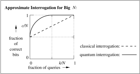
Figure 1: Comparison of the interrogation effectiveness between classical and quantum computers.

5 Conclusions

The model of quantum computation does not permit a general significant speed-up of the existing classical algorithms. Instead, we have to investigate for each different kind of problem whether there is a possible gain by using quantum algorithms or not.

Here it has been shown that for every binary function $\omega$ with domain size $N$, we can obtain the full description of the function with high probability while querying $\omega$ only $N/2+\sqrt{N}$ times. A classical computer always requires $N$ calls to determine $\omega_{1}\cdots\omega_{N}$ with the same kind of success probability.

The lower bounds on parity (with bounded error) and or (with no allowed error) for black-boxes[1, 6] show us that any quantum algorithm must use at least $N/2$ calls to obtain $\omega$ with bounded error, and that the full $N$ queries are necessary to determine the string without error, respectively. The question that remains therefore, is if the $\sqrt{N}$-term in the query complexity $N/2+\sqrt{N}$ is necessary or can perhaps be reduced to the order of $\log N$, for example.

The term ‘approximate interrogation’ was used for the scenario where we are interested in obtaining a certain fraction of the $N$ unknown bits. Again we could see how a quantum procedure outperforms the possible classical algorithms (Figure 1).

For all results in this article we assumed $\omega$ to be a random oracle without any structure. Future research on quantum computational complexity could investigate similar questions for structured oracles (the white-box model). This might lead to results that widen the gap between classical and quantum computation even further than we did here.

Appendix A Appendix: The Expected Number of Correct Bits for the Quantum Algorithm

In this appendix we will calculate how many bits we can expect to be correct for the quantum interrogation procedure with the initial state $\Psi$ of Equation 28. We do this by assuming that the unknown bit string consists of zeros only: $\vec{\omega}=0\cdots 0$. The expected number of correct bits for the algorithm equals therefore the expected number of zeros of the observed output string $\vec{y}$. Because we can make the assumption $\vec{\omega}=\vec{0}$ without loss of generality, we can then afterwards conclude that this number will the expected number of correct bits for any $\vec{\omega}$.

The inner-product between $\vec{x}$ and $\vec{\omega}$ will be zero for every $\vec{x}$, hence applying $A_{k}$ to $\Psi$ will not change the initial state:

$$A_{k}|\Psi_{k}^{\alpha}\rangle = \sum_{j=0}^{k}{\alpha_{j}\cdot\frac{1}{\sqrt{\left({\begin{array}[]{c}N\\ j\end{array}}\right)}}\sum_{\vec{x}\in\{0,1\}^{N}}^{\|\vec{x}\|=j}|\vec{x}\rangle}~{}.$$ (38)

After this $A_{k}$, we perform the $N$ Hadamard transforms on all $N$ qubits, yielding a new state:

$${H^{\otimes N}A_{k}|\Psi_{k}^{\alpha}\rangle} = \sum_{j=0}^{k}{\frac{\alpha_{j}}{\sqrt{\left({\begin{array}[]{c}N\\ j\end{array}}\right)}}\sum_{\vec{x}\in\{0,1\}^{N}}^{\|\vec{x}\|=j}H^{\otimes N}|\vec{x}\rangle}$$ (41)

$$= \frac{1}{\sqrt{2^{N}}}\sum_{\vec{y}\in\{0,1\}^{N}}\sum_{j=0}^{k}{\frac{\alpha_{j}}{\sqrt{\left({\begin{array}[]{c}N\\ j\end{array}}\right)}}\sum_{\vec{x}\in\{0,1\}^{N}}^{\|\vec{x}\|=j}{(-1)}^{(\vec{y},\vec{x})}|\vec{y}\rangle}$$ (44)

Because the above state is invariant under permutation, the probability of observing a certain string $\vec{y}$ depends only on its Hamming weight $\|\vec{y}\|$. This, in combination with some other known equalities[7] and mathematical techniques, enables us to express the expected number of zeros by

$$\textrm{\#zeros}({{H^{\otimes N}A_{k}|\Psi_{k}^{\alpha}\rangle}}) = \sum_{t=0}^{N}{t\cdot\left({\begin{array}[]{c}N\\ t\end{array}}\right){|\langle 0^{t}1^{N-t}|{H^{\otimes N}A_{k}|\Psi_{k}^{\alpha}\rangle}|}^{2}}$$ (47)

$$= \frac{N}{2}+\sum_{j=0}^{k-1}{\alpha_{j}\alpha_{j+1}\sqrt{j+1}\sqrt{N-j}}~{}.$$ (48)

We can therefore conclude that the expected number $c_{k}$ of correctly guessed bits for the quantum protocol will be (for given $k$ and $\alpha_{j}$):

$$c_{k}^{\mathrm{quant}} = \frac{N}{2}+\sum_{j=0}^{k-1}{\alpha_{j}\alpha_{j+1}\sqrt{j+1}\sqrt{N-j}}~{}.$$ (49)

References

- [1] R. Beals, H. Buhrman, R. Cleve, M. Mosca, and R. de Wolf. Quantum lower bounds by polynomials. In Proceedings of the 39th Annual Symposium on Foundations of Computer Science (FOCS’98). IEEE, 1998. Also as preprint on the quant-ph archive, no. 9802049.
- [2] C. Bennett and S. Wiesner. Communication via one- and two-particle operators on Einstein-Podolsky-Rosen states. Physical Review Letters, 69:2881–2884, 1992.
- [3] E. Bernstein and U. Vazirani. Quantum complexity theory. SIAM Journal on Computing, 26(5):1411–1473, 1997.
- [4] A. Berthiaume. Quantum computation. In A. L. Selman, editor, Complexity Theory Retrospective, In Honor of Juris Hartmanis on the Occasion of His Sixtieth Birthday, July 5, 1988, volume 2. Springer-Verlag, 1997.
- [5] R. Cleve, A. Ekert, C. Macchiavello, and M. Mosca. Quantum algorithms revisited. Proceedings of the Royal Society of London A, 454:339–354, 1998. Also as preprint on the quant-ph archive, no. 9708016.
- [6] E. Farhi, J. Goldston, S. Gutmann, and M. Sipser. A limit on the speed of quantum computation in determining parity, 1998. Preprint on the quant-ph archive, no. 9802045.
- [7] I. Gradshteyn and I. Ryzhik. Table of Integrals, Series, and Products. Academic Press, corrected and enlarged edition, 1965. Equalities 0.151.
- [8] L. Grover. Quantum computers can search arbitrarily large databases by a single query. Physical Review Letters, 79(23):4709–4712, Dec. 1997. Also as preprint on the quant-ph archive, no. 9706005.
- [9] A. Nayak and F. Wu. On the quantum black-box complexity of approximating the mean and the median, 1998. Preprint on the quant-ph archive, no. 9804066.
- [10] B. Terhal and J. Smolin. Single quantum querying of a database. Physical Review A, 58(3):1822–1826, Sept. 1998. Also as preprint on the quant-ph archive, no. 9705041.