Quantum Nonlocality without Entanglement

Abstract

We exhibit an orthogonal set of product states of two three-state particles that nevertheless cannot be reliably distinguished by a pair of separated observers ignorant of which of the states has been presented to them, even if the observers are allowed any sequence of local operations and classical communication between the separate observers. It is proved that there is a finite gap between the mutual information obtainable by a joint measurement on these states and a measurement in which only local actions are permitted. This result implies the existence of separable superoperators that cannot be implemented locally. A set of states are found involving three two-state particles which also appear to be nonmeasurable locally. These and other multipartite states are classified according to the entropy and entanglement costs of preparing and measuring them by local operations.

I Introduction

The most celebrated manifestations of quantum nonlocality arise from entangled states—states of a compound quantum system that admit no description in terms of states of the constituent parts. Entangled states, by their experimentally confirmed violations of Bell-type inequalities, provide strong evidence for the validity of quantum mechanics, and they can be used for novel forms of information processing, such as quantum cryptography [1], entanglement-assisted communication [2, 3], and quantum teleportation [4], and for fast quantum computations[5, 6], which pass through entangled states on their way from a classical input to a classical output. A related feature of quantum mechanics, also giving rise to nonclassical behavior, is the impossibility of cloning[7] or reliably distinguishing nonorthogonal states. Quantum systems that for one reason or another behave classically (e.g., because they are of macroscopic size or are coupled to a decohering environment) can generally be described in terms of a set of orthogonal, unentangled states.

In view of this, one might expect that if the states of a quantum system were limited to a set of orthogonal product states, the system would behave entirely classically, and would not exhibit any nonlocality. In particular, if a compound quantum system, consisting of two parts $A$ and $B$ held by separated observers (Alice and Bob), were prepared by another party in one of several mutually orthogonal, unentangled states, $\psi_{1},\psi_{2}...\psi_{n}$ unknown to Alice and Bob, then it ought to be possible to reliably discover which state the system was in by locally measuring the separate parts. Also, it ought to be possible to clone the state of the whole by separately duplicating the state of each part. We show that this is not the case, by exhibiting sets of orthogonal, unentangled states $\{\psi_{i}\}$ of two-party and three-party systems such that

• the states $\{\psi_{i}\}$ can be reliably distinguished by a joint measurement on the entire system, but not by any sequence of local measurements on the parts, even with the help of classical communication between the observers holding the separate parts;

• the cloning operation $\psi_{i}\rightarrow\psi_{i}\otimes\psi_{i}$ cannot be implemented by any sequence of local operations and classical communication.

Some of the features of this new kind of nonlocality appeared first in [8], which presented a set of orthogonal states of a bipartite system that cannot be cloned if Alice and Bob cannot communicate at all. However, the states in [8] can be cloned if Alice and Bob use one-way classical communication.

Many more of the nonlocal properties considered in the present work were anticipated by the measurement protocol introduced by Peres and Wootters[9]. Their construction indicates the existence of a nonlocality dual to that manifested by entangled systems: entangled states must be prepared jointly, but exhibit anomalous correlations when measured separately; the Peres-Wootters states are unentangled, and can be prepared separately, but exhibit anomalous properties when measured jointly. We note that such anomalies are at the heart of recent constructions for attaining the highest possible capacity of a quantum channel for the transmission of classical data[10, 11, 12, 13].

In the Peres-Wootters scheme, the preparator chooses one of three linear polarization directions 0, 60, or 120 degrees, and gives Alice and Bob each one photon polarized in that direction. Their task is to determine which of the three polarizations they have been given by a sequence of separate measurements on the two photons, assisted by classical communication between them, but they are not allowed to perform joint measurements, nor to share entanglement, nor to exchange quantum information.

Of course, because the three two-photon states are nonorthogonal, they cannot be cloned or reliably distinguished, even by a joint measurement. However, Peres and Wootters performed numerical calculations which provided evidence (more evidence on an analogous problem was provided by the work of Massar and Popescu[14]) indicating that a single joint measurement on both particles yielded more information about the states than any sequence of local measurements. Thus unentangled nonorthogonal states appear to exhibit a kind of quantitative nonlocality in their degree of distinguishibility. The discovery of quantum teleportation, incidentally, grew out of an attempt to identify what other resource, besides actually being in the same place, would enable Alice and Bob to make an optimal measurement of the Peres-Wootters states.

Another antecedent of the present work is a series of papers[15, 16, 17] resulting in the conclusion[17] that several forms of quantum key distribution[18] can be viewed as involving orthogonal states of a serially-presented bipartite system. These states cannot be reliably distinguished by an eavesdropper because she must let go of the first half of the system before she receives the second half. In this example, the serial time-ordering is essential: if, for example, the two parts were placed in the hands of two separate classically-communicating eavesdroppers, rather than being serially presented to one eavesdropper, the eavesdroppers could easily cooperate to identify the state and break the cryptosystem.

In this paper we report a form of nonlocality qualitatively stronger than either of these antecedents. We extensively analyze an example in which Alice and Bob are each given a three-state particle, and their goal is to distinguish which of nine product states, $\psi_{i}=|\alpha_{i}\rangle\otimes|\beta_{i}\rangle,i=1\ldots 9$ the composite $3\times 3$ quantum system was prepared in. Unlike the Peres-Wootters example, these states are orthogonal, so the joint state could be identified with perfect reliability by a collective measurement on both particles. However, the nine states are not orthogonal as seen by Alice or Bob alone, and we prove that they cannot be reliably distinguished by any sequence of local measurements, even permitting an arbitrary amount of classical communication between Alice and Bob. We call such a set of states “locally immeasurable” and give other examples, e.g., a set of two mixed states of two two-state particles (qubits), and sets of four or eight pure states of three qubits, which apparently cannot be reliably distinguished by any local procedure despite being orthogonal and unentangled.

In what sense is a locally immeasurable set of states “nonlocal?” Surely not in the usual sense of exhibiting phenomena inexplicable by any local hidden variable (LHV) model. Because the $\psi_{i}$ are all product states, it suffices to take the local states $\alpha_{i}$ and $\beta_{i}$, on Alice’s and Bob’s side respectively, as the local hidden variables. The standard laws of quantum mechanics (e.g. Malus’ law), applied separately to Alice’s and Bob’s subsystems, can then explain any local measurement statistics that may be observed. However, an essential feature of classical mechanics, not usually mentioned in LHV discussions, is the fact that variables corresponding to real physical properties are not hidden, but in principle measurable. In other words, classical mechanical systems admit a description in terms of local unhidden variables. The locally immeasurable sets of quantum states we describe here are nonlocal in the sense that, if we believe quantum mechanics, there is no local unhidden variable model of their behavior. Thus a measurement of the whole can reveal more information about the system’s state than any sequence of classically coordinated measurements of the parts.

The inverse of local measurement is local preparation, the mapping from a classically-provided index $i$ to the designated state $\psi_{i}$, by local operations and classical communication. If the states $\psi_{i}$ are unentangled, local preparation is always possible, but for any locally-immeasurable set of states this preparation process is necessarily irreversible in the thermodynamic sense, i.e., possible only when accompanied by a flow of entropy into the environment. Of course if quantum communication or global operations were allowed during preparation, the preparation could be done reversibly, provided that the states being prepared are orthogonal.

By eliminating certain states from a locally-immeasurable set (such as $\{\psi_{1},...\psi_{9}\}$ in Eq. (3) below), we obtain what appears to be a weaker kind of nonlocality, in which the remaining subset of states is both locally preparable and locally measurable, but in neither case (so far as we have been able to discover) by a thermodynamically reversible process. Curiously, in these situations, the entropy of preparation (by the best protocols we have been able to find) exceeds the entropy of measurement.

Besides entropies of preparation and measurement we have explored other quantitative measures of nonlocality for unentangled states. One obvious measure is the amount of quantum communication that would be needed to render an otherwise local measurement process reliable. Another is the mutual information deficit when one attempts to distinguish the states by the best local protocol. Finally one can quantify the amount of advice, from a third party who knows $i$, that would be sufficient to guide Alice and Bob through an otherwise local measurement procedure.

The results of this paper also have a bearing on, and were directly motivated by, a question which arose recently in the context of a different problem in quantum information processing. This is the problem of entanglement purification, in which Alice and Bob have a large collection of identical bipartite mixed states that are partially entangled. Their object is to perform a sequence of operations locally, i.e., by doing quantum operations on their halves of the states and communicating classically, and end up with a smaller number of pure, maximally entangled states. Recently, bounds on the efficiency of this process have been studied by Rains[19] and by Vedral and Plenio[20]; other constraints on entanglement purification by separable superoperators have recently been studied by Horodecki et al.[21].

In their work, they represent the sequence of operations using the theory of superoperators, which can describe any combination of unitary operations, interactions with an ancillary quantum system or with the environment, quantum measurement, classical communication, and subsequent quantum operations conditioned on measurement results. In the operator-sum representation of superoperators developed by Kraus and others, the general final state $\cal{S}(\rho)$ of the density operator of the system is written as a function of the initial state $\rho$ as:

$${\cal S}(\rho)=\sum_{k}S_{k}\rho S^{\dagger}_{k}.$$ (1)

The $S_{k}$ operators appearing in this equation will be referred to as “operation elements.” A trace-decreasing superoperator satisfies the condition $0\leq\sum_{k}S_{k}^{\dagger}S_{k}<1$ and is appropriate for describing the effect of arbitrary quantum measurements on the system ([22], Sec. III), while a trace-preserving superoperator specified by $\sum_{k}S_{k}^{\dagger}S_{k}=1$ describes a general time evolution of the density operator if a measurement is not made or its outcomes are ignored[23]. Reference [24] has a useful general review of the superoperator formalism.

To impose the constraint that Alice and Bob act only locally, Rains, and Vedral and Plenio, restricted their attention to separable superoperators, in which the operation elements have a direct product form involving an Alice operation and a Bob operation:

$$S_{k}=A_{k}\otimes B_{k}.$$ (2)

We will show in Sec. II B (see also [22], Sec. IX.C) that all operations that Alice and Bob can perform during entanglement purification bilocally, in which they can perform local quantum operations and communicate classically, can be written in this separable form. This was enough for the derivation of valid upper bounds on the efficiency of entanglement purification. But the natural question which this led to is the converse, that is, can all separable superoperators be implemented by bilocal operations?

The answer to this question is definitely no, as a result of the examples which we analyze in this paper. Quantum measurements are a subset of the superoperators, and measurements involving only product states are separable superoperators. Thus, our proof that some unentangled states cannot be distinguished locally shows that some separable superoperators cannot be implemented by only separate operations by Alice and Bob with classical communication between them. This indicates that any further investigations of entanglement purification protocols involving separable superoperators will have to be performed with some caution.

This paper is organized as follows: Section II presents the $3\times 3$ example and sketches the proof that these states cannot be distinguished by local measurements. Appendix B gives many of the important details of this proof, and Appendix A supplies a crucial technical detail, that all superoperators can be decomposed into a sequence of very weak measurements. Section III shows how the measurement can be done locally if some states are excluded, and presents the best measurement strategy we have found for distinguishing (imperfectly) all nine states. Section IV shows how the measurement can be done for the $3\times 3$ example if entanglement is supplied. Section V analyzes the thermodynamics of local state measurement, studying the heat generated in measurement and in state preparation; Appendix C gives some details. Section VI analyzes a three-party $2\times 2\times 2$ example involving 8 pure states. Section VII gives other compact examples (4 pure states in a $2\times 2\times 2$ system, 2 mixed states in a $2\times 2$ system) and poses some questions for the future (Appendix D gives details of a specific problem considered there).

II A separable measurement which is not bilocal

A The ensemble of states in a 3$\times$3 Hilbert space

We will consider the following complete, orthonormal set of product states $\psi_{i}=|\alpha_{i}\rangle\otimes|\beta_{i}\rangle$. They live in a nine-dimensional Hilbert space, with Alice and Bob each possessing three dimensions. We will use the notation $|0\rangle$, $|1\rangle$, and $|2\rangle$ for the bases of Alice’s and Bob’s Hilbert spaces. The orthonormal set is

$$\begin{array}[]{lll}&|\alpha\rangle{\mbox{}(Alice)}&|\beta\rangle{\mbox{}(Bob)}\\ \psi_{1}=&|1\rangle&|1\rangle\\ \psi_{2}=&|0\rangle&|0+1\rangle\\ \psi_{3}=&|0\rangle&|0-1\rangle\\ \psi_{4}=&|2\rangle&|1+2\rangle\\ \psi_{5}=&|2\rangle&|1-2\rangle\\ \psi_{6}=&|1+2\rangle&|0\rangle\\ \psi_{7}=&|1-2\rangle&|0\rangle\\ \psi_{8}=&|0+1\rangle&|2\rangle\\ \psi_{9}=&|0-1\rangle&|2\rangle.\end{array}$$ (3)

Here $|0\pm 1\rangle$ stands for ${1\over\sqrt{2}}(|0\rangle\pm|1\rangle)$, etc. Figure 1 shows a suggestive graphical way to depict the 9 states of Eq. (3) in the $3\times 3$ Hilbert space of Alice and Bob. The four dominoes represent the four pairs of states that involve superpositions of the basis states. State $\psi_{1}$ is clearly special in that it involves no such superposition.

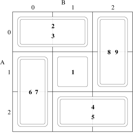
FIG. 1.: A graphical depiction of the nine orthogonal states of Eq. (3) as a set of dominoes.

B The measurement

We will show that the separable superoperator ${\cal S}(\rho)=\sum_{i}S_{i}\rho S_{i}^{\dagger}$ consisting of the projection operators

$$S_{i}=|i\rangle_{A}|i\rangle_{B}\langle\psi_{i}|$$ (4)

cannot be performed by local operations of Alice and Bob, even allowing any amount of classical communication between them. In Eq. (4), the output Hilbert space is different from the input; it is a space in which both Alice and Bob separately have a complete and identical record of the outcome of the measurement. See Sec. VII for a discussion of why we use the particular form of Eq. (4) for the operator; note that the input state need not be present at the output in Eq. (4).

Since this superoperator corresponds to a standard von Neumann measurement, we can equally well consider the problem in the form of the following game: Alice and Bob are presented with one of the nine orthonormal product states (for the time being, with equal prior probabilities, let us say—this is not important, it is only important that the prior probabilities of states $\psi_{2}$ through $\psi_{9}$ be nonzero). Their job is to agree on a measurement protocol with which they can determine, with vanishingly small error, which of the nine states it is, adhering to a bilocal protocol.

Let us characterize bilocal protocols a little more explicitly. Our discussion will apply both to bilocal measurements and to bilocal superoperators (in which the measurement outcomes may be traced out). By prior agreement one of the parties, let us say Alice, initiates the sequence of operations. The most general operation that she can perform locally is specified by the set of operation elements

$$A_{r1}\otimes I.$$ (5)

We will immediately specialize to the case where each value $r1$ labels a distinct “round 1” measurement outcome which she will report to Bob, since no protocol in which she withheld any of this information from Bob could have greater power. She cannot act on Bob’s state, so her operators are always the identity $I$ on his Hilbert space. $A_{r1}$ can also include any unitary operation that Alice may perform before or after the measurement. Note also that the operator $A_{r1}$ may not be a square matrix; the final Hilbert space dimension may be smaller (but this would never be useful) or larger (because of the introduction of an ancilla) than the original.

After the record $r1$ is reported to Bob, he does his own operation

$$I\otimes B_{r2}(r1).$$ (6)

The only change from round 1 is that Bob’s operations can be explicit functions of the measurements reported in that round. Now, the process is repeated. The overall set of operation elements specifying the net operation after $n$ rounds is given by multiplying out a sequence of these operations:

$$S_{m}=A_{m}\otimes B_{m},$$ (7)

$$A_{m}=A_{rn}(r1,r2,...,r(n-1))...A_{r3}(r1,r2)A_{r1},$$ (8)

$$B_{m}=B_{r(n-1)}(r1,r2,...,r(n-2))...B_{r4}(r1,r2,r3)B_{r2}(r1).$$ (9)

Here the label $m$ can be thought of as a concatenation of all the data collected through the $n$ rounds of measurement:

$$m=r1:r2:r3:...:rn.$$ (10)

Equations (7-9) demonstrate the fact that all bilocal operations are also separable operations. It is the converse statement that we are about to disprove for the operator corresponding to the nine-state measurement, Eq. (4).

We can get some intuitive idea of why it will be hard for Alice and Bob to perform Eq. (4) by local operations by noting the result if Alice and Bob perform simple, local von Neumann measurements in any of their rounds. These measurements can be represented on the “tic-tac-toe” board of Fig. 1 as simple horizontal or vertical subdivisions of the board. The fact that any such subdivision cuts apart one of the dominoes shows very graphically that after such an operation the distinguishability of the states is spoiled. This spoiling occurs in any local bases, and is more formally just a reflection of the fact that the ensemble of states as seen by Alice alone, or by Bob alone, is nonorthogonal.

However, it is not sufficient to show the impossibility of performing Eq. (4) using a succession of local von Neumann measurements, as Alice and Bob have available to them an infinite set of weak measurement strategies[25]. Much more careful reasoning is required to rule out any such strategy. In the remainder of this section we present the details of this proof, which also results in a computation of an upper bound on the amount of information Alice can Bob can obtain when attempting to perform the nine-state measurement bilocally.

C Summary of the proof

We assume that Alice and Bob have settled on a bilocal protocol with which they will attempt to complete the measurement as well as possible. We identify the moment in the execution of this measurement when Alice and Bob have accumulated a specific amount of partial information. We will have to show that it is always possible to identify this moment, either in Alice and Bob’s protocol or in an equivalent protocol which can always be derived from theirs. We then show, based on the specific structure of the nine states, that at this moment the nine possible input states must have become nonorthogonal by a finite amount. We then present an information-theoretic analysis of the mutual information obtainable in the complete measurement, and show, using an accessible-information bound, that the mutual information obtainable by Alice and Bob two-locally is less, by a finite amount, than the information obtained from a completely nonlocal measurement.

Now we present the steps of this proof in detail.

D Information accumulation and the modified continuous protocol

If the measurement has proceeded to a point where measurement record $m$ has been obtained, an inference can be made using Bayes’ theorem of the probability $p(\psi_{i}|m)$ that the input state was $\psi_{i}$:

$$p(\psi_{i}|m)={{p(m|\psi_{i})p(\psi_{i})}\over{\sum_{j}p(m|\psi_{j})p(\psi_{j})}}$$ (11)

We take all prior probabilities $p(\psi_{i})$ to be equal to $1\over 9$, so they will drop out of this equation. The measurement probabilities $p(m|\psi_{i})$ are given by the standard formula

$$p(m|\psi_{i})={\rm Tr}(S_{m}|\psi_{i}\rangle\langle\psi_{i}|S^{\dagger}_{m})=\langle\psi_{i}|S^{\dagger}_{m}S_{m}|\psi_{i}\rangle.$$ (12)

Here $S_{m}$ is the operation element of Eq. (7); the quantum state in Alice’s and Bob’s possession has been transformed to

$$\phi_{i,m}\equiv S_{m}|\psi_{i}\rangle.$$ (13)

We imagine monitoring these prior probabilities every time a new round is added to the measurement record in Eq. (10). We will divide the entire measurement into two stages, I and II; “stage I” of the measurement is declared to be complete when $p(\psi_{i}|m)$, for some $i$, equals a particular value (the choice of this value is discussed in detail in the next subsection). “Stage II” is defined as the entire operation from the end of stage I to the completion of the protocol.

There is a problem with this, however: the measurement record changes by discrete amounts on each round, and it is quite possible for these probabilities to jump discontinuously when a new datum is appended to this measurement record of Eq. (10). Thus, it is likely that the probabilities $p(\psi_{i}|m)$ will never attain any particular value, but will jump past it at some particular round. The probabilities would evolve continuously only if Alice and Bob agree on a protocol involving only weak measurements, for which all the $A_{rk}$ and $B_{rk}$ of Eqs. (8,9) are approximately proportional to the identity operator. But, in an attempt to thwart the proof about to be given, Alice and Bob may agree on a protocol which has both weak measurements and strong measurements (for which the operators of Eqs. (8,9) are not approximately proportional to the identity).

However, such a strategy will never be helpful for Alice and Bob, because, for any bilocal measurement protocol which they formulate involving any combination of weak and strong measurements, a modified measurement protocol exists that involves only weak measurements for which the amount of information extracted by the overall measurement is exactly the same. For this modified protocol an appropriate completion point for “stage I” of the measurement can always be identified. Thus we can prove, by the steps described below, that the modified protocol cannot be completed successfully by bilocal operations, and we give a bound on the attainable mutual information of such a measurement. But, since the modified protocol is constructed to have the same measurement fidelity as the original one, this proves that any protocol, involving any combination of weak and strong measurements, also cannot attain perfect measurement fidelity.

The modified protocol is created in a very simple way: it proceeds through exactly the same steps as the original protocol, except that at the point where the result of a strong measurement is about to be reported to the other party by transmission through the classical channel, the strong measurement record, treated as a quantum-mechanical object, is itself subjected to a long sequence of very weak measurements. The outcomes of these weak measurements are reported, one at a time, to the other party and appended to the measurement record in Eq. (10).

The precise construction of this weak-measurement sequence is described in Appendix A. The weak measurements are designed so that in their entirety they give almost perfect information about the outcome of the strong measurement (the strong measurement outcome itself can be reported at the end of this sequence as a confirmation). So, the recipient of this steam of reports from the outcomes of the weak measurements need only wait until they are done to know the actual (strong) measurement outcome in order to proceed with the next step of the original protocol. But, except in cases with vanishingly small probability, the information contained in the accumulating measurement record grows continuously.

To conclude this discussion of the modified measurement protocol, we can show how Alice and Bob can be duped into being unwitting participants in the modified protocol, and also give an illuminating if colloquial view of how the “continuumization” of the measurement can take place. What is required is a modification of the makeup of the classical channel between Alice and Bob. We imagine that when Alice transmits the results of a measurement, thinking that it is going directly into the classical channel to Bob, it is actually intercepted by another party (Alice’), who performs the necessary sequence of weak measurements. Here is a way that Alice’ can implement this operation: She examines the bit transmitted by Alice. If the bit is a 0, she selects a slightly head-biassed coin, flips it many times, each time transmitting the outcome into the classical channel. If the bit is a 1, she does the same thing with a slightly tail-biassed coin. At the other end of the channel there is another intercepting agent (Bob’) who, after studying a long enough string of coin flips sent by Alice’, can with high confidence deduce the coin bias and report the result to Bob. Alice and Bob are oblivious to this whole intervening process; nevertheless, as measured by the data actually passing through the channel, the modified protocol with nearly continuous evolution of the available information has been achieved.

E The state of affairs after stage I of the measurement

Having established that no matter what Alice and Bob’s measurement protocol, we can view the probabilities as evolving continuously in time, we can declare that stage I of the measurement is complete when

$$\max_{i}\ p(\psi_{i}|m_{I})={1\over 9}+\epsilon,$$ (14)

that is, after the probabilities have evolved by a small but finite amount away from their initial value of $1\over 9$. It should be noted that since some measurement outcomes might be much more informative than others, the time of completion of stage I is not fixed; it will in general require a greater number of rounds for one measurement record $m_{I}$ than for another.

The $\epsilon$ in Eq. (14) should be some definite, small, but noninfinitesimal number. Moreover, we will require that all posterior probabilities $p(\psi_{i}|m_{I})$ be nonzero. For this any value smaller than $1\over 72$ will be acceptable, since

$$\min_{i}\ p(\psi_{i}|m_{I})\geq{1\over 9}-8\epsilon.$$ (15)

We now rewrite Bayes’ theorem from Eq. (11):

$$p(\psi_{i}|m_{I})={{\langle\psi_{i}|E_{m_{I}}|\psi_{i}\rangle}\over{\sum_{j}\langle\psi_{j}|E_{m_{I}}|\psi_{j}\rangle}}={{\langle\alpha_{i}|a_{m_{I}}|\alpha_{i}\rangle\langle\beta_{i}|b_{m_{I}}|\beta_{i}\rangle}\over{\sum_{j}\langle\psi_{j}|E_{m_{I}}|\psi_{j}\rangle}}.$$ (16)

Here we have introduced an abbreviated notation for several operators which will come up repeatedly in the upcoming derivations:

$$\begin{array}[]{l}E_{m_{I}}=S^{\dagger}_{m_{I}}S_{m_{I}}=a_{m_{I}}\otimes b_{m_{I}},\\ a_{m_{I}}=A^{\dagger}_{m_{I}}A_{m_{I}},\\ b_{m_{I}}=B^{\dagger}_{m_{I}}B_{m_{I}}.\end{array}$$ (17)

Where there is no risk of confusion we will drop the index $m_{I}$ from $E_{m_{I}}$, $a_{m_{I}}$, and $b_{m_{I}}$.

It is easy to bound the greatest possible spread in the probability distribution:

$${{8+72\epsilon}\over{8-9\epsilon}}\leq\max_{i,j}{{p(\psi_{i}|m_{I})}\over{p(\psi_{j}|m_{I})}}=\max_{i,j}{{\langle\alpha_{i}|a|\alpha_{i}\rangle\langle\beta_{i}|b|\beta_{i}\rangle}\over{\langle\alpha_{j}|a|\alpha_{j}\rangle\langle\beta_{j}|b|\beta_{j}\rangle}}\leq{{1+9\epsilon}\over{1-72\epsilon}}.$$ (18)

An important technical consequence of declaring stage I complete at this point is that it is guaranteed that all the matrix elements $\langle\alpha_{i}|a|\alpha_{i}\rangle$ and $\langle\beta_{i}|b|\beta_{i}\rangle$ are nonzero; this condition will be used repeatedly in the analysis of Appendix B (to be described shortly). The more crucial condition from Eq. (18) is that either the following equation is true,

$$\max_{i,j}{{\langle\alpha_{i}|a|\alpha_{i}\rangle}\over{\langle\alpha_{j}|a|\alpha_{j}\rangle}}\geq\sqrt{{8+72\epsilon}\over{8-9\epsilon}},$$ (19)

or the corresponding equation for $b$ is true. This says that either the operator $a$ or $b$ differs from being proportional to the identity operator by a finite amount. This will be the key fact in the analysis we are about to report.

The basic idea is that at the completion of stage I, from Alice’s and Bob’s point of view there is a nonzero probability that the initial state was any one of the nine. In order for Alice and Bob to complete the job of identifying which state they have been given—with a reliability approaching 100%—it is necessary that the nine states remaining after stage I, Eq. (13), still be almost perfectly distinguishable. That is, the states must still be nearly orthogonal. But we can show that, because of Eq. (19), these residual states cannot be sufficiently orthogonal to complete the task. In fact, we will be able to compute exactly to what extent they must be nonorthogonal. For we can show that, if we assume that the overlap of any two of these residual states is $\delta$ or less, i.e.,

$$\max_{i,j}\ \langle\phi_{i,m_{I}}|\phi_{j,m_{I}}\rangle=\max_{i,j}{{|\langle\psi_{i}|a\otimes b|\psi_{j}\rangle|}\over{\sqrt{\langle\psi_{i}|a\otimes b|\psi_{i}\rangle\langle\psi_{j}|a\otimes b|\psi_{j}\rangle}}}=\delta,$$ (20)

then both $a$ and $b$ will both be almost proportional to the identity operator, with relative corrections proportional to $\delta$. This is done in Appendix B where these corrections are derived precisely. The important consequence of this is that

$$\max_{i,j}{{\langle\alpha_{i}|a|\alpha_{i}\rangle}\over{\langle\alpha_{j}|a|\alpha_{j}\rangle}}\leq 1+O(\delta),$$ (21)

and the same for $b$. Equations (19) and (21) cannot be both satisfied unless $\delta=O(\epsilon)$, that is, unless the residual states are nonorthogonal by a finite amount.

So, at this point we can conclude that the measurement Eq. (4) cannot be done bilocally, except with less that 100% accuracy; this is the main result that we set out to prove. We now proceed to a more quantitative analysis of bilocal approximations to this measurement.

F Information-theoretic analysis of the two-stage measurement

We can now perform an analysis of the precise effects of this nonorthogonality, and derive an upper bound on the information attainable by Alice and Bob from any bilocal protocol. We will use the standard classical quantifier of information, the mutual information[26], which gives the amount of knowledge of one random variable (in our case, the identity of quantum state $\psi_{i}$) gained by having a knowledge of another (here, the outcome of the measurement).

Recall that we have broken the measurement by Alice and Bob into two stages. We will call the random variable describing the stage-I outcomes $M_{I}$. The outcomes of all subsequent (stage-II) measurements will be denoted by random variable $M_{II}$. Alice and Bob’s object is to deduce perfectly the label $i$ of one of the nine states $\psi_{i}$ (Eq. (3)); we will use the symbol $W$ for this random variable (for “which wavefunction”). We quantify the information attainable in the measurement by the mutual information $I(W;M_{I},M_{II})$ between $W$ and the composite measurement outcomes $M_{I}$ and $M_{II}$. For a perfect measurement, the attainable mutual information is $\log_{2}9$; we will show that $I(W;M_{I},M_{II})$ must be less than this. We first use the additivity property of mutual information ([26], p. 125) to write:

$$I(W;M_{I},M_{II})=I(W;M_{II}|M_{I})+I(W;M_{I}).$$ (22)

This expression introduces the mutual information between $W$ and $M_{II}$ conditional on $M_{I}$, which can be written as an average over all the possible outcomes $m_{I}$ of the measurement in stage I:

$$I(W;M_{II}|M_{I})=\sum_{m_{I}}p(m_{I})I(W;M_{II}|m_{I}).$$ (23)

Now, combining Eqs. (22,23) with the definition of the mutual information:

$$I(W;M_{I})=H(W)-H(W|M_{I}),$$ (24)

and using the fact that the entropy of the initial distribution $H(W)=\log_{2}9$, we obtain

$$I(W;M_{I},M_{II})=\log_{2}9-\sum_{m_{I}}p(m_{I})(H(W|m_{I})-I(W;M_{II}|m_{I})).$$ (25)

To show that Eq. (25) must be less than $\log_{2}9$ it will be sufficient to show that each member of the sum is strictly positive. The conditions at the end stage I make it possible for us to do this.

To make things explicit, let us suppose that at the end of stage I the residual quantum states (recall Eq. (13)) $\rho_{i}=|\phi_{i,m_{I}}\rangle\langle\phi_{i,m_{I}}|$ occur with probabilities $q_{i}=p(\psi_{i}|m_{I})$ from Eq. (16). (There will be no confusion from leaving out the $m_{I}$ label.) Moreover, let us suppose that the measurement to be performed in stage II corresponds to a positive operator-valued measure $\{M_{b}\}$ fixed by measurement outcome $m_{I}$. Then the explicit expression for the mutual information $I(W;M_{II}|m_{I})=I(M_{II};W|m_{I})$ becomes

$$I(M_{II};W|m_{I}) = H(M_{II}|m_{I})-H(M_{II}|W,m_{I}),$$ (26)

$$= -\sum_{b}({\rm tr}\,\rho M_{b})\log_{2}({\rm tr}\,\rho M_{b})+\sum_{i=1}^{9}q_{i}\sum_{b}({\rm tr}\,\rho_{i}M_{b})\log_{2}({\rm tr}\,\rho_{i}M_{b})\;,$$ (27)

where $\rho=\sum_{i}q_{i}\rho_{i}$. Note that $H(W|m_{I})=-\sum_{i=1}^{9}q_{i}\log_{2}q_{i}$.

Without loss of generality for the present set of manipulations, let us take $\phi_{1,m_{I}}$ and $\phi_{2,m_{I}}$ to be the two states assured to have a nonvanishing overlap $\langle\phi_{1,m_{I}}|\phi_{2,m_{I}}\rangle=\delta$ (recall Eq. (20)). We may partition the density operator $\rho$ according to the two states that interest us most as follows. Let

$$\tau_{1}=\sum_{i=1}^{2}\frac{q_{i}}{s_{1}}\rho_{i}\qquad\mbox{and}\qquad\tau_{2}=\sum_{i=3}^{9}\frac{q_{i}}{s_{2}}\rho_{i}$$ (28)

where $s_{1}=q_{1}+q_{2}$ and $s_{2}=1-s_{1}$. We can think of this partition as generating two new “which wavefunction” random variables $W_{1}$ and $W_{2}$—the probabilities associated with these random variables are just the renormalized ones appearing in Eq. (28). Note that $\rho=s_{1}\tau_{1}+s_{2}\tau_{2}$. Then, by the classic converse to the concavity of the Shannon entropy ([27], p. 21), it follows that

$$-\sum_{b}({\rm tr}\,\rho M_{b})\log_{2}({\rm tr}\,\rho M_{b})\leq-s_{1}\sum_{b}({\rm tr}\,\tau_{1}M_{b})\log_{2}({\rm tr}\,\tau_{1}M_{b})-s_{2}\sum_{b}({\rm tr}\,\tau_{2}M_{b})\log_{2}({\rm tr}\,\tau_{2}M_{b})+h(s_{1})\;,$$ (29)

where $h(x)=-x\log_{2}x-(1-x)\log_{2}(1-x)$ is the binary entropy function. Hence, if we write

$$I(M_{II};W_{1}|m_{I}) = -\sum_{b}({\rm tr}\,\tau_{1}M_{b})\log_{2}({\rm tr}\,\tau_{1}M_{b})+\sum_{i=1}^{2}\frac{q_{i}}{s_{1}}\sum_{b}({\rm tr}\,\rho_{i}M_{b})\log_{2}({\rm tr}\,\rho_{i}M_{b})\;,$$ (30)

$$I(M_{II};W_{2}|m_{I}) = -\sum_{b}({\rm tr}\,\tau_{2}M_{b})\log_{2}({\rm tr}\,\tau_{2}M_{b})+\sum_{i=3}^{9}\frac{q_{i}}{s_{2}}\sum_{b}({\rm tr}\,\rho_{i}M_{b})\log_{2}({\rm tr}\,\rho_{i}M_{b})\;,$$ (31)

it follows that

$$I(M_{II};W|m_{I})\leq s_{1}I(M_{II};W_{1}|m_{I})+s_{2}I(M_{II};W_{2}|m_{I})+h(s_{1})\;.$$ (32)

We can further bound this, so as to remove all dependence on states $\phi_{3,m_{I}}$ through $\phi_{9,m_{I}}$, by noting that

$$I(M_{II};W_{2}|m_{I})\leq H(W_{2}|m_{I})=-\sum_{i=3}^{9}\frac{q_{i}}{s_{2}}\log_{2}\frac{q_{i}}{s_{2}}\;.$$ (33)

Combining Eqs. (32) and (33) gives

$$H(W|m_{I})-I(W;M_{II}|m_{I})\geq-\sum_{i=1}^{2}q_{i}\log_{2}q_{i}+s_{1}\log_{2}s_{1}-s_{1}I(M_{II};W_{1}|m_{I})\;.$$ (34)

Equation (34) can be further bounded so as to remove any explicit dependence on $q_{1}$ and $q_{2}$ by noting that, for fixed $s_{1}$, the first term in the expression on the right-hand side is minimized when $q_{1}=q_{2}$. (One can verify this simply by taking a derivative respect to one of the free variables.) Making that restriction, one can see furthermore that the resultant term is monotonically increasing in $q_{1}$. Thus the bound we are looking for can be found by taking $q_{1}$ to be its minimal allowed value, namely $q_{1}=\beta={1\over 9}-8\epsilon$ (recall Eq. (15)). With all that in place, we have that

$$H(W|m_{I})-I(W;M_{II}|m_{I})\geq 2\beta\!\left[1+\sum_{b}({\rm tr}\,\tau_{1}M_{b})\log_{2}({\rm tr}\,\tau_{1}M_{b})-\sum_{i=1}^{2}\frac{1}{2}\sum_{b}({\rm tr}\,\rho_{i}M_{b})\log_{2}({\rm tr}\,\rho_{i}M_{b})\right]\;,$$ (35)

where now $\tau_{1}=\frac{1}{2}(\rho_{1}+\rho_{2})$.

Finally it is a question of removing all dependence on the quantum measurement $\{M_{b}\}$. This can be gotten by noting that the two right-most terms in the right-hand side Eq. (35) simply correspond to the mutual information given by the measurement $\{M_{b}\}$ about the two equiprobable nonorthogonal quantum states $\phi_{1,m_{I}}$ and $\phi_{2,m_{I}}$ (cf. Eq. (30)). Optimizing over all quantum measurements, we obtain the accessible information of those two states [28]. Inserting that into Eq. (35) and recalling Eq. (20) we finally find,

$$H(W|m_{I})-I(W;M_{II}|m_{I})\geq 2\beta\,h({1\over 2}-{1\over 2}\sqrt{1-\delta^{2}})=({2\over 9}-16\epsilon)h({1\over 2}-{1\over 2}\sqrt{1-\delta^{2}}),$$ (36)

where $h(x)$ is again the binary entropy.

The last bound can be made useful by establishing a quantitative link between $\epsilon$ and $\delta$ in Eq. (36). To do this, we must identify the value of $\delta$ for which, given all the constraints derived in Appendix B, it is first possible to satisfy Eq. (19) for some values of $i$ and $j$. It is this value of $\delta$ which must be used in the bound Eq. (36). We have exhaustively examined all $i,j$ pairs to determine which one allows the greatest ratio of $a$ (or $b$) matrix elements for a given value of $\delta$. We find this to be the case for $i=8$ and $j=6$ in Eq. (3) (or other symmetry-equivalent ones). For this choice we can write

$${{\langle x_{8}|a|x_{8}\rangle}\over{\langle x_{6}|a|x_{6}\rangle}}={{a_{00}+a_{11}+2{\rm Re}\,a_{01}}\over{a_{11}+a_{22}+2{\rm Re}\,a_{12}}}.$$ (37)

This ratio attains its maximum value when

$$a_{00}=a_{11}\frac{1+\delta}{1-\delta}\;,\quad a_{22}=a_{11}\frac{1-\delta}{1+\delta}\;,\quad{\rm Re}\,a_{01}=a_{11}\nu_{\epsilon}\sqrt{\frac{1+\delta}{1-\delta}}\;,\quad{\rm Re}\,a_{12}=-a_{11}\nu_{\epsilon}\sqrt{\frac{1-\delta}{1+\delta}}$$ (38)

These are the extremal values permitted by Eqs. (B11) and (B37). The value this gives is

$$\max_{i,j}{{\langle\alpha_{i}|a|\alpha_{i}\rangle}\over{\langle\alpha_{j}|a|\alpha_{j}\rangle}}\leq f_{\epsilon}(\delta)=\left({{1+\delta}\over{1-\delta}}\right){{1+\nu_{\epsilon}\sqrt{1-\delta^{2}}}\over{1-\nu_{\epsilon}\sqrt{1-\delta^{2}}}}.$$ (39)

The smallest value of $\delta$ for which Eqs. (19) and (39) are consistent is given by the solution to the equation

$$f_{\epsilon}(\delta)=\sqrt{{8+72\epsilon}\over{8-9\epsilon}}.$$ (40)

Using Mathematica, we have found the choice of $\epsilon$ and $\delta$ consistent with Eq. (40) that gives the strongest bound on the mutual information in Eq. (36). We obtain:

$$I(W;M_{I},M_{II})\leq\log_{2}9-\Delta,$$ (41)

where the mutual-information deficit $\Delta=0.00000531$. This upper bound is attained when $\epsilon=0.00823$, corresponding to a nonorthogonality parameter $\delta=0.00344$ and a minimum-probability parameter $\beta=0.0453=(0.408)/9$. Thus, we bound the information attainable by bilocal operations by Alice and Bob away from that attainable in a fully nonlocal measurement by a minute but finite amount.

III Searching for Optimal Local Measurements

Equation (41) gives our upper bound on the mutual information one can obtain by means of local operations and classical communication. However, it is unlikely that this bound is a close approximation to the actual optimal mutual information accessible in this way; most likely the optimal value is significantly lower. In this section we explore specific measurement strategies for our nine-state ensemble in order to get a sense of how well one can in fact distinguish the states by local means. We will thereby obtain a lower bound on the mutual information.

We begin by considering a simpler problem, namely, distinguishing only eight of the nine states from each other. That is, we consider the case where the prior probability of one of the states is zero.

As we noted earlier, state $\psi_{1}$ from Eq. (3) is special. In fact, it is never used in the analysis of Appendix B; thus, its presence or absence is irrelevant to the nonorthogonality conditions which we have derived. This means that this state is not necessary to make the measurement undoable bilocally. Thus, even if we take the prior probabilities of the states such that $p(\psi_{1})=0$, we will still reach the conclusion that the full mutual information is unattainable by a bilocal procedure (the quantitative analysis will be different than that given above).

The same is not true for the other states: if the prior probability of any of the states $\psi_{2}$-$\psi_{9}$ is zero, then the measurement can be completed successfully by Alice and Bob. Figures 2 and 3 illustrate this for the case when the state $\psi_{4}$ is left out. One way of explaining the strategy is that since the 4-5 domino of Fig. 2 is no longer complete, it can be cut by a von Neumann measurement, which will disturb state $\psi_{5}$ but still leave it distinguishable from all the other eight states. Thus, the protocol can begin with cut 1 of Fig. 2, which corresponds to an incomplete von-Neumann measurement by Bob which distinguishes his state $|2\rangle$ from states $|0\rangle$ or $|1\rangle$ (but does not distinguish between $|0\rangle$ and $|1\rangle$). The next step to be taken by Alice depends on the reported outcome as received by her from Bob, as indicated by the tree of Fig. 3; likewise all four rounds of the measurement are similarly contingent on the measurement outcomes of preceding rounds. The object at every round is to move towards isolating a domino so that its pair of states can be distinguished by a measurement in the rotated basis.

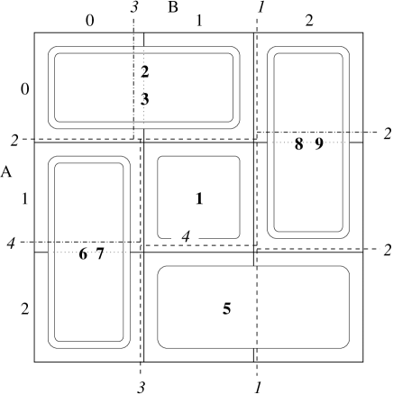
FIG. 2.: The sequence of measurements performed to distinguish the states of Fig. 1 if state $\psi_{4}$ is excluded. The dashed lines indicate the von Neumann measurements, the italic numbers indicate the order in which they are performed. Dash-dotted lines indicate measurements in the rotated basis.

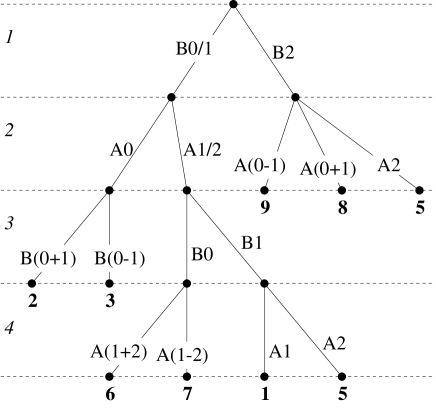
FIG. 3.: A tree depicting the four states of measurement indicated in Fig. 2. “A” and “B” indicate the party performing the measurement. B0/1 indicates that the 0 and 1 outcomes are not distinguished. The bold-faced numbers at the base of the tree indicate the states which are inferred from this chain of measurements.

We now turn to our original problem of distinguishing optimally among all nine states, assumed to have equal prior probabilities. The measurement strategy just described is a reasonable one to pursue even when all nine states are present. It accurately distinguishes states $\psi_{1-3}$ and $\psi_{6-9}$, and it distinguishes these states from $\psi_{4}$ and $\psi_{5}$; it fails only to distinguish these last two states from each other. (In applying Fig. 3 to this case, one should imagine replacing “5” with “4 or 5.”) Thus if Alice and Bob use this measurement, then with probability $\frac{7}{9}$ they obtain the full $\log_{2}9$ bits of information, and with probability $\frac{2}{9}$ they are left one bit short; so the mutual information is $\log_{2}9-\frac{2}{9}$ = 2.9477 bits. One can, however, do better, and we now present a series of improvements over the above strategy.

We may express the improved measurements as sequences of positive operator-valued measures (POVMs). For example, Bob could start with a POVM consisting of elements $b_{r1}$ (these are 3$\times$3 matrices that must satisfy the constraint $\sum_{r1}b_{r1}=I$), after which Alice will perform a measurement $\{a_{r2}\}$, and so on. As it happens, all of our improved measurements can be represented in terms of POVMs whose elements are diagonal in the standard bases for Alice and Bob. It is therefore convenient to represent these POVM elements by their diagonal values. For example, in the measurement described above, Bob’s opening POVM (in this case a von Neumann measurement), which distinguishes his state $|2\rangle$ from $|0\rangle$ and $|1\rangle$, has two elements which we represent as $\{1,1,0\}$ and $\{0,0,1\}$.

Our first improvement is to replace this von Neumann measurement by a more symmetric POVM whose elements are $b_{1}=\{1,\frac{1}{2},0\}$ and $b_{2}=\{0,\frac{1}{2},1\}$. (If Bob were to perform this measurement when his part of the system was in the central state $|1\rangle$, the outcome would be random.) Note that each outcome of this measurement rules out one of the columns of Fig. 1; that is, it rules out one of Bob’s states $|0\rangle$ or $|2\rangle$. Once this has been done, Alice may freely cut either the 6-7 domino or the 8-9 domino, and from this point Bob and Alice may proceed as above to find out (with no further damage) in which domino the actual state lies. However, Bob’s initial measurement damages both the 2-3 domino and the 4-5 domino, so that at the end, he will not be able to distinguish perfectly between $\psi_{2}$ and $\psi_{3}$ or between $\psi_{4}$ and $\psi_{5}$. Thus, in order to evaluate the mutual information obtainable via this strategy, we need to know the effect of Bob’s initial POVM on these four states. This effect depends on what operation element $B_{r1}$ we choose to associate with the POVM element $b_{r1}$. Any $B_{r1}$ satisfying $B_{r1}^{{\dagger}}B_{r1}=b_{r1}$ is allowed, but it is simplest to let $B_{r1}$ be $|r1\rangle\otimes\sqrt{b_{r1}}$, where $|r1\rangle$ is the classical record of the outcome. To see how this measurement affects the states, let us suppose that the actual state is $\psi_{4}$, so that Bob’s part of the system begins in the state $|\phi\rangle=\frac{1}{\sqrt{2}}(|1\rangle+|2\rangle)$. Then if Bob gets the outcome $b_{1}$, the final state of Bob’s part of the system (not including the classical record) is $\sqrt{b_{1}}|\phi\rangle=\frac{1}{2}|1\rangle$, and if he gets the outcome $b_{2}$ the final state is $\sqrt{b_{2}}|\phi\rangle=\frac{1}{2}|1\rangle+\frac{1}{\sqrt{2}}|2\rangle$. (These states are automatically subnormalized so that their squared norms are the probabilities of the corresponding outcomes, namely, $\frac{1}{4}$ and $\frac{3}{4}$.) If the initial state had been $\psi_{5}$, then the results would have been the same but with $|2\rangle$ replaced by $-|2\rangle$. Thus the first outcome renders $\psi_{4}$ and $\psi_{5}$ completely indistinguishable, while the second merely makes them non-orthogonal. In the latter case Bob can, at the end, try to determine whether the original state was $\psi_{4}$ or $\psi_{5}$ by performing the optimal measurement for distinguishing two equally likely non-orthogonal states [28]. In this case the optimal measurement is simply the orthogonal measurement whose outcomes are B($1+2$) and B($1-2$). Similar considerations apply to the states $\psi_{2}$ or $\psi_{3}$. One finds that this strategy yields a mutual information of 2.9964 bits, which is an improvement over the strategy of Fig. 3.

A further improvement is gained by replacing Bob’s initial POVM by a less informative and less destructive one whose elements are $\{p,\frac{1}{2},1-p\}$ and $\{1-p,\frac{1}{2},p\}$, where $\frac{1}{2}<p<1$. The rest of the measurement is left unchanged. Optimizing over $p$, one finds that this strategy can yield 3.009 bits of mutual information. Note, however, that in this case Bob’s initial measurement does not rule out any column of Figure 1, so that when Alice later cuts a domino, she may be cutting the actual state, in which case her action will cost them one bit. One may suspect that Alice should be more careful, and indeed the mutual information is improved if she makes a weaker measurement. In fact, the best strategy we have found delays until the fourth round a measurement that guarantees the complete cutting of a domino.

This best strategy consists of the following steps, in which the values of the parameters $p,q,r,s,$ and $t$ are to be determined by optimization:

1. Bob: $\{p,\frac{1}{2},1-p\}$ vs $\{1-p,\frac{1}{2},p\}$. Let us assume that Bob gets the first outcome. (In the other case all the POVM elements appearing in the succeeding steps have their diagonal values reversed; that is, the roles of states $|0\rangle$ and $|2\rangle$ are interchanged.)

2. Alice: $\{0,1-q,1-r\}$ vs $\{1,q,r\}$. The first outcome cuts the 8-9 domino, and we go directly to step 5. The second outcome makes it safer for Bob to risk cutting the 4-5 domino, so we proceed to step 3.

3. Bob: $\{1-s,1-t,0\}$ vs $\{s,t,1\}$. The first outcome cuts the 4-5 domino, and we go directly to step 5. The second outcome makes it safer for Alice to cut the 6-7 domino, so we proceed to step 4.

4. Alice: $\{1,1,0\}$ vs $\{0,0,1\}$. Either outcome cuts the 6-7 domino.

5. At this point some domino has been cut, so that Alice and Bob can proceed as above to determine in which domino the actual state lies. If this domino contains two states that have not been collapsed into the same state, Alice and Bob then perform a measurement to try to distinguish them.

Optimizing over the values of the parameters, we find that the mutual information is $\log_{2}9-0.1575=3.0125$ bits. (One set of parameter values giving this result is $p=0.726,\,q=0.395,\,r=0.312,\,s=0.071,\,t=0.104$.) Moreover, numerical evidence indicates that no further advantage is gained by allowing another round before making a firm cut (it would be a cut of the 2-3 domino, as we proceed clockwise around the grid). Thus it is conceivable that this value of the mutual information is indeed optimal, though we cannot rule out an entirely different strategy that does better.

Summarizing the results of this Section and the preceding one, we have

$$\log_{2}9-0.1575\leq I(W;M_{I},M_{II})\leq\log_{2}9-\Delta.$$ (42)

Note that the results presented in this section can be seen as a realization of the ideas behind our proof in Section II. Alice and Bob begin by performing a sequence of POVMs aimed at determining in which domino the actual state lies; this sequence can be thought of as stage I of the measurement. At this point, just as in our proof, the states remaining to be distinguished have become non-orthogonal, so that the final mutual information must fall short of $\log_{2}9$ bits.

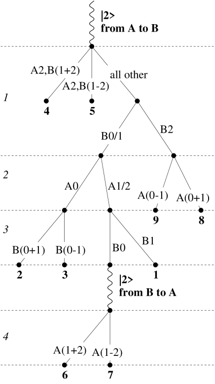
FIG. 4.: A modification of the tree of Fig. 3 which shows how all nine states can be reliably distinguished with some quantum communication from Alice to Bob. The wavy lines indicate the episodes of quantum transmission; the first transmission permits Bob to locally do a measurement involving both A and B pieces of the Hilbert space.

IV A realization of the two-party separable superoperator with shared qubits

Having established that the measurement can only be done approximately if Alice and Bob only communicate classically, it is natural to ask what quantum resources would permit them to complete the measurement. It is obvious that they can do it if Alice ships her entire 3-state system to Bob and he performs the full operation in his lab, reporting the result classically back to Alice. In the case of all 9 states having equal prior probability, this requires the transmission of $\log_{2}3\approx 1.58496$ qubits. If state $\psi_{1}$ is left out and the other 8 states are equiprobable, the density matrix of the state held by Alice has less than maximal entropy, in fact it has $h_{3}({3\over 8},{2\over 8},{3\over 8})={11\over 4}-\log_{2}3\approx 1.16504$ bits of entropy. Using the Schumacher compression theorem[29], this means that if Alice and Bob are performing many shots of the same measurement on states drawn from the same ensemble, then the quantum transmission from Alice and Bob can be compressed to $1.16504$ qubits per shot.

However, in the nine-state case we can exhibit a protocol for completing the measurement which requires a smaller overall number of qubits transmitted. It starts with the imperfect protocol involving only classical communication just discussed (Fig. 4), and adds a part to permit states 4 and 5 to be perfectly distinguished. This will require only $h({1\over 3})+{2\over 9}\approx 1.14152$ qubits (over many repetitions of the measurement). For the 8-state case the protocol will actually be worse than the straightforward one, requiring $h({3\over 8})+{2\over 8}\approx 1.20443$ qubits of transmission. In neither case do we know that the procedures which we discuss here are optimal.

The modified protocol for the 9-state case begins with Alice transmitting the $|2\rangle$ component of her Hilbert space to Bob. It is obvious that she could do this by sending 1 qubit, if she adopts a 3-qubit unary encoding of her Hilbert space, i.e., $|0\rangle\rightarrow|100\rangle$, $|1\rangle\rightarrow|010\rangle$, and $|2\rangle\rightarrow|001\rangle$. In fact the third qubit in this representation has less than maximal entropy, having entropy $h({1\over 3})$ (it has higher entropy, $h({3\over 8})$, for the 8-state case). Thus, again using Schumacher’s theorem[29], the transmission can be compressed over many realizations of the measurement so that only $h({1\over 3})$ of a qubit per measurement needs to be transmitted.

As indicated by the tree in Fig. 4, Bob’s possession of $|2\rangle_{A}$ permits him to immediately do a measurement which distinguishes whether the state is $\psi_{4}$, $\psi_{5}$, or is one of the others. After this has been done the sequence of measurements proceeds identically as in the classical protocol (Fig. 4), except that some possibilities can be pruned off as they correspond to $\psi_{4}$ and $\psi_{5}$ cases which have already been distinguished. Before completing round 4, Alice must be again in possession of $|2\rangle_{A}$, which requires a qubit transmission back from Bob. This qubit is not compressible, but this transmission will only be required if the state is $\psi_{6}$ or $\psi_{7}$, which will only happen $2\over 9$ of the time, and will count as $2\over 9$ qubits of transmission ($2\over 8$ for the 8-state case).

Adding up the qubit transmissions at the beginning and the end of Fig. 4 gives $h({1\over 3})+{2\over 9}\approx 1.14152$ qubits as mentioned above. This transmission can be made unidirectional, since a qubit sent in one direction, if it is entangled with a qubit left behind, may always be used to teleport a qubit in the opposite direction[4]. Note that even with the assistance of qubit transmissions, this protocol requires several rounds of classical transmission; it is a true “two-way” protocol, that is, requiring bidirectional classical communication[30].

V Thermodynamics of nonlocal measurements and state preparation

A Irreversibility of measurement

We now explore another information-theoretic feature of our two-party measurement that illustrates in another way the nonlocality of this orthogonal measurement. If the parts of the quantum states are assembled in one location, then a measurement in any orthogonal basis, in addition to being doable with 100% fidelity, can be done reversibly. That is, the quantum state can be converted into classical data without any discarding of information to the environment. Therefore by Landauer’s principle [31] no heat is generated during the measurement. The reversible method can be illustrated by a simple qubit example: if the measurement is to distinguish $|0\rangle$ from $|1\rangle$, and the classical record of the bit is to be stored in the macro states $|\underline{0}\rangle\equiv|000...\rangle$ and $|\underline{1}\rangle\equiv|111...\rangle$ (containing, say, $10^{23}$ qubits), then the procedure involves starting the macro system in a standard state (so that the initial states of the system to be measured is either $|0000...\rangle$ or $|1000...\rangle$), then performing repeated quantum XOR operations[30] with the qubit to be measured as the source and all the qubits of the macro state as the targets. In the end, the measured qubit may as well be considered to be part of the macro system containing the classical answer. Note that no interaction with any other environment is necessary to complete this, or any other, local orthogonal measurement.

The situation is rather different for our two-party orthogonal measurement. Suppose that we consider a case in which the measurement can be achieved by Alice and Bob, for example the case in which state $\psi_{4}$ is promised not to be present. Although Alice and Bob can perform this measurement, they clearly cannot do so reversibly, i.e., as a finite sequence of local reversible operations and classical communications. In the protocol described in Fig. 2, the irreversibility arises in the first step, where, if the state is $\psi_{5}$, it is irreversibly transformed to either state $|2\rangle|1\rangle$ or to $|2\rangle|2\rangle$. Thus in this case 1 bit of entropy is produced. If each of the eight permitted states occurs with equal probability, then the average entropy generated is $1\over 8$ of a bit. We cannot prove this entropy of measurement is minimal, though we have found no more efficient protocol. Many other cases can be easily worked out; for example, if it is promised that the state is only one of four (say, $\psi_{6}$, $\psi_{2}$, $\psi_{8}$, and $\psi_{4}$), then $1\over 4$ of a bit of entropy will be generated by the obvious protocol.

It appears that reversible measurements are only possible if the set of states can be progressively dissected by Alice and Bob without breaking any dominoes. To formalize this notion, we introduce a few definitions. Let $S=\{\psi_{i}\}$ be a set of pure product states shared between Alice and Bob, where $\psi_{i}=\alpha_{i}\otimes\beta_{i}$. Given such a set, we define a splitting of $S$ by Alice as a partition of $S$ into two nonempty disjoint subsets $S=S_{1}\cup S_{2}$ such that for all $\psi_{i}\in S_{1}$ and for all $\psi_{j}$ in $S_{2}$, $\langle\alpha_{i}|\alpha_{j}\rangle=0$. A splitting by Bob is defined similarly. A set $S$ is dissectible if there is a tree each of whose interior nodes is a splitting by Alice or Bob and whose leaves are singletons. For example, using the numbering of Eq. (3) and Fig. 1, the set $\{\psi_{2},\psi_{6},\psi_{8}\}$ is dissectible, but $\{\psi_{2},\psi_{4},\psi_{6}\,\psi_{8}\}$ is not. The dissectibility of an arbitrary set $S$ can be determined by examining finitely many possible splitting trees. Clearly any subset of a dissectible set is dissectible. It is evident that if an ensemble of states ${\cal E}=\{p_{i},\psi_{i}\}$ has support only on a dissectible set, then both its entropy of preparation and entropy of measurement are zero. It is tempting to argue that, conversely, nondissectible sets, if they are locally measurable at all, have positive entropies of measurement, but to be sure of this, one would have to exclude the (unlikely-seeming) possibility of multi-step measurement procedures which, while not strictly reversible for any finite $n$, would succeed in identifying each of the states in the nondissectible set with error probability and entropy production both tending to 0 in the limit of large $n$.

A further analysis of this irreversibility reveals that it can be thought of as originating in the necessity for classical communication between Alice and Bob. In order to assure that the channel between them can convey only classical and no quantum information, the channel itself must possess a quantum environment (in order to dephase the data passing though it). This raises the possibility that Alice or Bob will be obliged to become entangled with the environment of the channel in the course of communicating the necessary classical information, thereby causing themselves to have a finite amount of entropy. Exactly the same amount must also appear in the channel environment. When, for example, Alice and Bob have been given state $\psi_{5}=|2\rangle\otimes(|1\rangle+|2\rangle)$, and Bob sends the result of his first measurement in Fig. 3 (collapsing his state to a mixture of $|1\rangle$ and $|2\rangle$) to Alice, he has created entanglement between the measurement outcome and the environment, so that the joint system of message and environment is left an entangled state of the form $|1\rangle\otimes e_{1}+|2\rangle\otimes e_{2}$, where $e_{1}$ and $e_{2}$ are two orthogonal states of the environment.

Note that measurement protocols requiring classical communication are not inevitably irreversible. For example, for the dissectible set $\{\psi_{2},\psi_{6},\psi_{8}\}$ considered previously, a bit of communication from Bob to Alice is required to complete the measurement; still no entropy is generated. This is so because this bit is guaranteed to be in one of the computational basis states, precisely the states with which the dephasing channel does not entangle. It is the necessity, in the above example, of delivering a bit to the channel which is in a superposition of basis states which leads to the entanglement and the irreversibility.

B Irreversibility of state preparation

For dissectible sets of states, such as $\{\psi_{2},\psi_{6},\psi_{8}\}$, the mapping

$$|i\rangle\otimes|i\rangle\leftrightarrow|\alpha_{i}\rangle\otimes|\beta_{i}\rangle,$$ (43)

(using the notation of Eq. (3)) between classical instructions and the state described is locally reversible and can be performed in either direction without the generation of waste information. Conversely, nondissectible sets, such as $\{\psi_{2},\psi_{4},\psi_{6},\psi_{8}\}$, cannot be prepared by any finite sequence of reversible operations, and we conjecture that even asymptotic multistep protocols could not reduce either the heat of preparation or the heat of measurement to zero. Perhaps surprisingly, the heats of preparation and measurement, by the best protocols we have been able to discover, are unequal.

To give an example of irreversible state preparation, consider the following method for the preparation for the nondissectible set $\{\psi_{2},\psi_{4},\psi_{6},\psi_{8}\}$ mentioned above. The protocol, which is the best we know, will produce $h({1\over 4})\approx 0.811$ bits of entropy, considerably more than the entropy of measurement. The procedure works as follows: First, Bob computes a function $f$ of the preparation instruction $i$ which records whether the state to be synthesized is $\psi_{4}$ ($f(4)=1$) or one of the others ($f(2,6,8)=0$), saving the result in a work bit. Then Alice and Bob reversibly prepare the modified four states of Fig. 5; that is, if the instruction is to prepare $\psi_{4}$, $\psi_{4^{\prime}}$ is prepared, and in the other three cases exactly the desired state is produced.

This preparation can be carried out reversibly because the modified set $\{\psi_{2},\psi_{4}^{\prime},\psi_{6},\psi_{8}\}$ is dissectible. Next, Bob performs a Hadamard rotation on his state ($|2\rangle\rightarrow|1+2\rangle$, $|1\rangle\rightarrow|1-2\rangle$, $|0\rangle\rightarrow|0\rangle$) conditional upon the state of $f(i)$, which transforms $4^{\prime}$ into $4$ and leaves the other three states unchanged as desired. Finally Bob erases his work bit $f(i)$, which requires discarding $h({1\over 4})$ bits of entropy into the environment. Similar reasoning shows that the equiprobable nine-state ensemble can be prepared at a cost of $h({2\over 9})\approx 0.764$, and the equiprobable eight-state ensemble (without the center state) at a cost of $h({2\over 8})\approx 0.811$ bits of entropy.

It should perhaps be noted that the local preparation and measurement protocols we have described, while irreversible from the viewpoint of Alice and Bob, become reversible when viewed from a global perspective, including Bob, Alice and the environment. In the preparation protocol we have just described this global reversibility arises because the waste classical information $f(i)$ discarded into the environment in the last step is not random, but instead is entirely determined by the joint state $\psi_{i}$ of Alice and Bob. Therefore discarding it, though it increases the entropy of the environment, does not increase the entropy of the universe. The global reversibility of the measurement protocol for this same set of four states arises because the information discarded into the environment in the final stage is merely the other half of the entanglement created at an earlier stage of the protocol, when one of the dominoes might have been collapsed. Thus the final act of discarding restores the environment to a pure state.

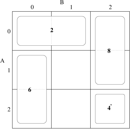
FIG. 5.: A set of four states, shown in the domino notation, which can be prepared locally by Alice and Bob in a reversible fashion.

When speaking of the thermodynamic costs of local preparation and local measurement, it should be recalled that, although any set of product states can be locally prepared, not all sets can be locally measured. The full set of nine states $\{\psi_{1}...\psi_{9}\}$ of Eq. (3), for example, is not locally measurable at all, no matter how much heat generation is allowed. Conversely, there are sets of pure bipartite states that cannot be prepared locally, even with the generation of heat, because one or more states in the set is entangled. The concepts of entropy of preparation and entropy of measurement can nevertheless be extended to such sets, indeed to any orthogonal set of pure bipartite states, by allowing Alice and Bob to draw on a reservoir of prior entanglement (e.g., standard singlets $\Psi^{-}={1\over\sqrt{2}}(|01\rangle-|10\rangle)$ shared between them) to help perform actions, such as teleportation[4], that could not otherwise be done locally. In this fashion one can define an entanglement-assisted entropy of local preparation, and an entanglement-assisted entropy of local measurement. In entanglement-assisted measurement, an otherwise immeasurable set like the original set of nine states is rendered measurable by teleporting quantum information as required, say, in the protocol of Fig. 4. However, each teleportation generates two bits of waste classical information per qubit teleported, thereby contributing to the entropy of measurement. Again we can calculate the amounts of entanglement consumed and entropy produced by simple protocols, without knowing whether more efficient ones exist. The protocols described earlier give an entanglement-assisted entropy of measurement of 2.28304 bits for the equiprobable nine-state ensemble, and 2.40886 bits for the eight-state ensemble (omitting the central state), in each case twice the amount of entanglement consumed, because the protocols generate no other waste information aside from that associated with the teleportations. Turning now to entanglement-assisted preparation, a typical set of states requiring entanglement to prepare from classical directions is set of four Bell states[30] $\{\Phi^{+},\Phi^{-},\Psi^{+},\Psi^{-}\}$. The entropy of preparation by the obvious protocol in this case is two bits per state prepared (Bob reads the classical directions, applies an appropriate Pauli rotation to the standard $\Psi^{-}$ to make the desired Bell state, then throws away the classical directions).

Finally suppose Alice and Bob are given an unknown member of the 9-state set (or some other locally-immeasurable set) and wish to determine which state they have without the help of entanglement, but with some hints from a person who knows which state they have been given. We define the “advice of measurement” as the minimal amount of advice needed (in conjunction with their own local actions) to guide Alice and Bob to the right answer. As we have seen above, a negative hint like “the state is not $\psi_{4}$” is sufficient. This might appear to be a lot of advice (as much as a totally informative positive hint like “the state is $\psi_{3}$,”) but in fact such negative hints are highly compressed by classical hashing techniques, asymptotically requiring only ${8\over 9}\log_{2}{8\over 7}\approx 0.171\,$ bits per hint in the nine-state case. Appendix C gives details of the compression of these types of hints.

We note, however, that the non-von Neumann measurements discussed at the end of section III allow an even more efficient form of advice. There it was shown that an appropriate POVM yields $3.0125=\log 9-0.1575$ bits of information about the unknown state in the 9-state case; therefore, after Alice and Bob have performed their POVM, only 0.1575 bits of additional information need be provided asymptotically for them to identify the state exactly.

As an aside, we note that the value of advice, and the amount needed, may depend on its timing. Although in the 9-state measurement problem the most efficient advice we know of can safely be given at the end, after the POVM has been completed, there are other situations in quantum information theory, not to mention in everyday life, when early advice is more useful than late advice. In the BB84 quantum key distribution protocol[18], for example, the basis information may be regarded as a form of advice that is delayed to make it less useful to the eavesdropper. In a deterministic setting, where the adviser can foresee all future events, nothing is lost by giving all necessary advice at the beginning. But when unforeseen events are possible, the most efficient kind of advice, better than prior or posterior advice, may be as-needed or concurrent advice. Suppose Alice and Bob are about to begin a long car trip. They ask their more experienced friend Eve which route to take. A few days later they telephone again, asking her how to repair a flat tire. To be helpful, the route advice must be given at the beginning, but it would be wasteful to give the repair advice then because the flat tire might not have happened. The prominent role of measurements, whether von Neumann or POVM, with unpredictable outcomes, in our analysis of the 9-state problem suggests that as-needed advice might be the optimal kind here also.

The notion of advice of measurement can be extended to sets of entangled states as well, for example the set of four Bell states. Here one bit of advice is sufficient (e.g., whether the unknown Bell state is of the $+$ or $-$ type), since the other bit ($\Phi$ vs. $\Psi$) can be learned by comparing the results of local measurements in the $z$ basis. The table summarizes the various measures of nonlocality for some of the ensembles we have been considering.

Ensemble	9-state	2468	246	4-Bell	2-Bell
Locally Preparable	Yes	Yes	Yes	No	No
Locally Measurable	No	Yes	Yes	No	Yes
Dissectible	No	No	Yes	No	No
Entropy of Prep.	0.764	0.811	0	2	1
Entropy of Meas.	2.283	0.250	0	2	1
Entanglement of Prep.	0	0	0	1	1
Entanglement of Meas.	1.142	0	0	1	0
Advice of Meas.	0.1575	0	0	1	0

Notes: Entropies, entanglements, and advice for non-Bell ensembles are upper bounds from known protocols—actual values could be less. Entropy of measurement for 9-state and 4-Bell ensembles are for entanglement-assisted measurement, since these ensembles are otherwise not locally measurable. The nine-state ensemble consists of 9 equiprobable states $\psi_{1}...\psi_{9}$ of Eq. (3) and Fig. 1. The 2468 and 246 ensembles are equiprobable distributions over $\{\psi_{2},\psi_{4},\psi_{6},\psi_{8}\}$ and $\{\psi_{2},\psi_{4},\psi_{6}\}$ respectively. The 4-Bell ensemble consists of four equiprobable Bell states $\{\Phi^{+},\Phi^{-},\Psi^{+},\Psi^{-}\}$, and the 2-Bell ensemble of two equiprobable Bell states, e.g., $\{\Phi^{+},\Psi^{+}\}$.

VI A three-party separable superoperator

We shall now show another example of a separable von Neumann measurement, this time involving three parties, Alice, Bob and Carol, each holding just a qubit (two-state system). While we have not performed a full analysis of this case, it appears to have the same properties as the 9-state measurement above—that partial measurement causes indistinguishability of the residual states—suggesting that this is another case in which the measurement cannot be done locally by the three parties, even if the three can partake in any amount of classical communication among themselves. The superoperator involves a complete orthonormal set of eight product states living in the eight-dimensional Hilbert space. This appears to be the smallest possible Hilbert space which still presents such behavior (it is easy to show, using a simple elimination process, that a qubit-trit system or a qubit-qubit system is not sufficient). The eight states are:

$$\begin{array}[]{llllr}&{\mbox{}Alice}&{\mbox{}Bob}&{\mbox{}Carol}\\ \phi_{1}=&|0\rangle&|0\rangle&|0\rangle&\,\,\,\,\,=\ \verb\phi_{2}=&|1\rangle&|1\rangle&|1\rangle&=\ \verb\phi_{3}=&|0+1\rangle&|0\rangle&|1\rangle&=\ \verb\phi_{4}=&|0-1\rangle&|0\rangle&|1\rangle&=\ \verb\phi_{5}=&|0\rangle&|1\rangle&|0+1\rangle&=\ \verb\phi_{6}=&|0\rangle&|1\rangle&|0-1\rangle&=\ \verb\phi_{7}=&|1\rangle&|0+1\rangle&|0\rangle&=\ \verb\phi_{8}=&|1\rangle&|0-1\rangle&|0\rangle&=\ \verb$$ (44)

(leaving out normalizations). On the right side of these equations we introduce an obvious shorthand for these states which we will use in the Discussion. We will indicate the evidence that the separable superoperator consisting of the projection operators

$$S_{i}=|i\rangle_{A}|i\rangle_{B}|i\rangle_{C}\langle\phi_{i}|$$ (45)

cannot be performed by 3-local operations, in which Alice, Bob, and Carol can only perform local quantum operations and broadcast classical information to each other.

The arguments are equivalent to those in the two-trit example, and again rely on considering any measurement as a two-stage process. In the case where all prior probabilities are equal ($1\over 8$ in this case), we declare stage I to be complete when

$$\max_{i}p(\phi_{i}|m_{I})={1\over 8}+\epsilon,$$ (46)

with some positive $\epsilon$ smaller than $1\over 56$, It is again simple to bound the greatest possible spread of the probability distribution:

$${{7+56\epsilon}\over{7-8\epsilon}}\leq\max_{i,j}{{p(\phi_{i}|m_{I})}\over{p(\phi_{j}|m_{I})}}=\max_{i,j}{{\langle\phi_{i}|E|\phi_{i}\rangle}\over{\langle\phi_{j}|E|\phi_{j}\rangle}}\leq{{1+8\epsilon}\over{1-56\epsilon}}.$$ (47)

As before, this equation guarantees that all diagonal matrix elements of $E$, $\langle\phi_{i}|E|\phi_{i}\rangle=\langle\phi_{i}|a\otimes b\otimes c|\phi_{i}\rangle$, are nonzero, and it also guarantees that the maximum and minimum matrix elements are different. Also as before, we can show that the states after stage I become nonorthogonal, which should permit us to derive a definite mutual-information deficit. We will not develop this proof here, but we will give a simple sketch of how we prove that the states are nonorthogonal. We will just show here that the states cannot be exactly orthogonal:

$$|\langle\phi_{j}|a\otimes b\otimes c|\phi_{i}\rangle|=0,\;\;\;\;\forall i\neq j.$$ (48)

This proof can be generalized step by step into a full analysis as in Appendix B.

1) Writing the orthogonality condition for $i=3$ and $j=4$ gives condition that

$$(a_{00}+a_{01}-a_{10}-a_{11})b_{00}c_{11}=0.$$ (49)

Since diagonal matrix elements of $b$ and $c$ must be nonzero by the arguments from Eq. (47), the $a$ factor must be zero; taking the real part gives

$$a_{00}=a_{11}.$$ (50)

2) Taking taking $i=5$ and $j=6$ and applying the same reasoning gives

$$c_{00}=c_{11}.$$ (51)

3) And taking $i=7$ and $j=8$ gives

$$b_{00}=b_{11}.$$ (52)

4) Now we write the four orthogonality conditions coming from all combinations of $i=3,4$ and $j=5,6$:

$$\begin{array}[]{rcl}(a_{00}+a_{01})b_{01}(c_{10}+c_{11})&=&0\\ -(a_{00}+a_{01})b_{01}(c_{10}-c_{11})&=&0\\ (a_{00}-a_{01})b_{01}(c_{10}+c_{11})&=&0\\ -(a_{00}-a_{01})b_{01}(c_{10}-c_{11})&=&0.\end{array}$$ (53)

Adding these four equations gives

$$4a_{00}b_{01}c_{11}=0.$$ (54)

Since $a_{00}\neq 0$ and $c_{11}\neq 0$, we conclude that

$$b_{01}=0=b_{10}.$$ (55)

5) Doing the same for the equations involving $i=3,4$ and $j=7,8$ gives

$$c_{01}=0=c_{10}.$$ (56)

6) And finally from the equations involving $i=5,6$ and $j=7,8$, we get

$$a_{01}=0=a_{10}.$$ (57)

Putting observations 1) through 6) together, we conclude that $a$, $b$ and $c$ must be proportional to the identity operator. But this is inconsistent with Eq. (47), which established that the different diagonal matrix elements of $E$ must differ by a finite amount. When developed more fully, this result should contradict the assumption that the measurement could be done even approximately by 3-local operations.

Note that nothing in the argument involves the simple product states $\phi_{1}$ or $\phi_{2}$. We conclude that the measurement is still not doable locally even if these two states are promised to be absent. On the other hand, it is easy to show that eliminating any one of the states $\phi_{3-8}$ would permit the measurement to be done. The layout of these states in the Hilbert space shown in Fig. 6 gives some intuition for why these should be true, as in the two-party case: any simple von Neumann involves cutting one of these “dumbbells” and making those pairs of states indistinguishable.

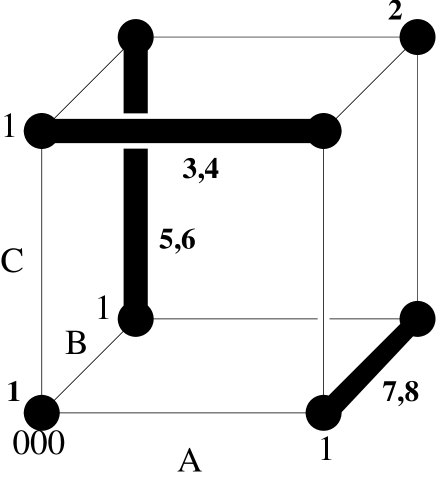
FIG. 6.: The layout of the eight states of Eq. (44) in the $2\times 2\times 2$ Hilbert space. The “dumbbells” have a similar meaning as the dominoes in Fig. 1.

Finally, the most economical technique that we have found for making the measurement doable with quantum communication is for a whole qubit to be sent from one party to another. That is, no compression of the quantum information seems to be possible in this case, whether or not states $\phi_{1}$ or $\phi_{2}$ are excluded. It is easy to show that the resulting two-party measurement which is required after this qubit transmission is doable by local actions.

VII Discussion

The results of this paper, extensive as they are, raise many additional fundamental questions about multipartite quantum measurements, most of which we have only incomplete answers to at this time. We would indeed be pleased if the ambitious reader has a notion of how to attack any of the following puzzles:

There are a variety of simple variants on the separable measurements presented in this paper for which we do not know how to prove or disprove bilocality. One is a very obvious generalization of the 9-state example:

$$\begin{array}[]{lll}&{\mbox{}Alice}&{\mbox{}Bob}\\ \psi^{\prime}_{1}=&\;\;\;|1\rangle&\;\;\;|1\rangle,\\ \psi^{\prime}_{2}=&\;\;\;|0\rangle&\;\;\;\cos\theta_{23}|0\rangle+\sin\theta_{23}|1\rangle,\\ \psi^{\prime}_{3}=&\;\;\;|0\rangle&-\sin\theta_{23}|0\rangle+\cos\theta_{23}|1\rangle,\\ \psi^{\prime}_{4}=&\;\;\;|2\rangle&\;\;\;\cos\theta_{45}|2\rangle+\sin\theta_{45}|1\rangle,\\ \psi^{\prime}_{5}=&\;\;\;|2\rangle&-\sin\theta_{45}|2\rangle+\cos\theta_{45}|1\rangle,\\ \psi^{\prime}_{6}=&\;\;\;\cos\theta_{67}|2\rangle+\sin\theta_{67}|1\rangle&\;\;\;|0\rangle,\\ \psi^{\prime}_{7}=&-\sin\theta_{67}|2\rangle+\cos\theta_{67}|1\rangle&\;\;\;|0\rangle,\\ \psi^{\prime}_{8}=&\;\;\;\cos\theta_{89}|0\rangle+\sin\theta_{89}|1\rangle&\;\;\;|2\rangle,\\ \psi^{\prime}_{9}=&-\sin\theta_{89}|0\rangle+\cos\theta_{89}|1\rangle&\;\;\;|2\rangle.\end{array}$$ (58)

That is, each of the domino pair is rotated by a different angle. While we strongly doubt that the case of general $\theta$s is any different from the case $\theta=\pi/4$ that we have analyzed, we have no proof that these general states specify a nonlocal measurement.

We have noted that, although there is no $2\times 2$ pure-state example that involves pure states of a separable but nonlocal superoperator, there is a mixed-state measurement which has some very curious properties. It is a measurement to distinguish two density matrices $\rho_{0}$ and $\rho_{1}$, where $\rho_{0}$ is an equal mixture of the pure product states 0+ and +0 (we use the notation introduced in Eq. (44)) and $\rho_{1}$ is an equal mixture of 11 and --. It appears that, despite the fact that this measurement involves distinguishing two separable, orthogonal states, nevertheless the measurement cannot be done bilocally, indeed, the measurement apparently cannot be done by any separable superoperator! It is easy to show that the projection measurement into these states can produce an entangled output from an unentangled input (for instance, 0(0++)); no separable superoperator can do this. It will be interesting to understand the minimum degree of nonlocality needed to perform this measurement.

A nonlocal measurement would yield 1 bit of information since $\rho_{0}$ and $\rho_{1}$ are orthogonal. It would be interesting to try to apply the techniques developed in this paper to determine a bound on the attainable mutual information by a bilocal approximation to this measurement.

There are other multi-party examples for which such proofs would also be desirable. A modified version of the $2\times 2\times 2$ example above involves just four states:

$$\verb$$ (59)

$$\verb$$ (60)

$$\verb$$ (61)

$$\verb$$ (62)

These states do not correspond to a separable trace-preserving superoperator, as the complement to these four measurements is not separable[32]. Nevertheless, this can be viewed as a measurement game in which Alice, Bob, and Carol are promised that they are given one of these four states, and their object is to distinguish, with only classical communications, which state it is. We suspect that they cannot, but we have not been able to prove it.

An even more exotic set of orthogonal states that we have considered is one involving 10 parties, each with a qubit. This set of states again only involves basis vectors 0, 1, +, and - locally, so that a typical one of the 1024 basis states is 1+-+0--110. This construction emerges from a counterexample of a proposition in tiling theory, the Keller conjecture[33]. The violation of this conjecture means that the 1024 states do not conform to the domino or dumbbell layout of the examples in this paper, where pairs of dimensions of the Hilbert space are covered by pairs of orthogonal states. We have not attempted to prove non-10-locality for this example, but we note that there is no simple von Neumann measurement that will distinguish them.

Curiously, despite the complexity of the example, we are able to show that just two copies of any state are sufficient for the 10 parties to be able to locally distinguish the state with classical communication, as in all the examples considered in Sec. IV. The procedure is simple: measure one copy in the 0/1 basis, and the second in the +/- basis. This has raised another question: are there any sets of states, entangled or not, for which some finite number greater than 2 of copies of the state is necessary for distinguishing the states reliably? So far we have found no examples where more than two copies of the unknown state are needed[34]. Indeed we know of no examples of two orthogonal pure states, product or entangled, which require more than one copy to be relibaly distinguished. Earlier in this section we noted a set of two orthogonal mixed states of two qubits which appears to be locally immeasurable. But here too, two copies are sufficient to make the states distinguishable. It would appear that further work on the tiling problems could produce other interesting examples for numbers of parties between 3 and 10.

The domino representation of two-party quantum states bears some resemblance to an approach taken in classical communication complexity problems to finding the most efficient interactive scheme for evaluating a function of data held by both Alice and Bob with the minimum classical communication[35]. The resemblance comes when the one-bit output of the function is depicted in a two-dimensional table; then the most efficient communication is determined by a recursive subdivision of such a table into unanimous blocks. It remains to be seen whether this observation would lead to more examples of interesting separable quantum operations.

The present investigation has required a very precise distinction between different types of quantum operations which are normally considered identical. Going back to the 9-state calculation, we can consider two different quantum operations related to the measurement operation of Eq. (4) (repeated here):

$$|i\rangle_{A}|i\rangle_{B}\langle\psi_{i}|,$$ (63)

$$|\psi_{i}\psi_{i}\rangle\langle\psi_{i}|,$$ (64)

$$|\psi_{i}\rangle\langle\psi_{i}|.$$ (65)

We have disproved the existence of (63). We can from this disprove the existence of (64), which is a cloning operator: we just note that Alice and Bob could perform this cloning many times, then perform measurements to deduce with very high confidence the state label $i$, thus performing (63). We can also rule out any form of weak cloning[36]. The case for (65) is more subtle, since we normally think of these projection operators as precisely what we mean by the measurement (63). This is true in a one-party world, since performing the projection means that a classical record of the state is available somewhere in the world. But in a multi-party situation, this record could be in a form which is split between the parties in a way which would require quantum communication to unravel. Therefore, we emphatically state that (63) and (65) are not generally identical in a multi-party scenario. Indeed, we note that there is another case in which two such operators are completely different. For Bell states, the measurement operator Eq. (63) cannot be done bilocally, because of the entanglement of the states; but the dephasing operator Eq. (65) for the Bell states can be done bilocally; it has been described as the “twirling” operation of Ref. [30].

Nevertheless, we have been able to prove that (65) is not doable for the 9-state examples, but by quite different arguments than those given for Eq. (63), presented in Appendix D. But the issue of approximations to (65), or (64), remains unsettled. That is, we do not know how to quantify the precision with which Alice and Bob could do these operations approximately. A large part of the difficulty is that we cannot use a simple, classical measure of information like the mutual information, which was possible for (63) because the output is a classical record. For (64) and (65) an operator measure, involving a notion of distance between two quantum operators, would have to be used. The theory of such operator measures is considerably less well developed[37].

It seems likely that the states we have explored in this paper would be usable for quantum cryptography, but we also have more questions than answers on this point. It is now clear[17] that bipartite orthogonal states are generally useful for cryptography when one particle in the state is received by Bob before the other has been launched by Alice. This forces Eve to measure one particle at a time. If Eve had no quantum memory, then the security of the cryptography protocol would be assured if the measurement of the state could not be performed bilocally, with the restriction that only round of measurement (one transmission from Alice to Bob) would be permitted. The nine states that we have analyzed have this property. However, given that Eve can have a quantum memory, the problem is a bit different, corresponding to there being some restricted form of quantum communication between Alice and Bob in the measurement protocol. In the cryptographic application, of course, Eve has more work to do: she must determine the identity of the state and provide it undisturbed, at the appropriate times, to Bob[38]. Thus, a separate study is required to establish that the nine states form a good basis for orthogonal quantum cryptography (which, however, is easily provided by the analysis of [17]). At the same time, we may imagine that the nine states might provide a stronger cryptographic primitive for some purposes, given that they cannot be identified even by repeated communication between Alice and Bob. Another useful feature of the states as a cryptographic primitive might be the fact that two copies of them can be identified exactly. But we have no concrete notions of what these new cryptographic applications might be.

Finally, we note that the basic question which began our investigation remains unanswered: what is a compact mathematical description of a superoperator which can be performed by only classical communication between the parties? We have only disproved one natural hypothesis, that this set coincides with the set of separable superoperators. No alternative hypothesis has presented itself.

All of these questions indicate, we think, that we still have many very basic questions about the structure of quantum mechanics, about the nature of quantum nonlocality and of entanglement, questions whose answers will be of central significance in our quest to employ quantum mechanics in the transmission and processing of information.

A Decomposition of arbitrary POVM into a series of very weak measurements

Any superoperator acting on a system of dimension $n$ can be replaced (nonuniquely) by the following procedure: appending an ancilla of dimension $n_{1}$, performing a unitary transformation, tracing out a subsystem of dimension $n_{2}$, and measuring (using a standard and complete measurement) a subsystem of dimension $n_{3}$, which we call a probe. As a result, the state of remaining system (of dimension $m=\frac{nn_{1}}{n_{2}n_{3}}$) can be calculated, and it is uniquely determined for any given superoperator despite of the nonuniqueness of the procedure. In cases where there is no probe to be measured ($n_{2}=1$), this is the so-called trace-preserving superoperator. If instead the trace-out step is eliminated, this is the most general POVM (positive operator-valued measurement). In our case, where all information is used for the optimal extraction of information, we are interested in this second case. Thus, the most general POVM can be replaced by the three operations – the appending of an ancilla, the unitary transformation and the standard measurement of a subsystem.

Suppose we are given a state, on which we will obtain some information using a POVM. We will show how to approximate this POVM by a continuous process. The addition of ancilla does not influence the state; the unitary transformation can be done as continuously as we wish. We shall now show that a standard complete measurement can be replaced by a continuous process (to any desired approximation). As a result of the above discussion, any POVM can be approximated in the same way.

In order to measure the probe (a subsystem of dimension $n_{3}$) using a complete standard measurement in a basis $|i\rangle$, we write the combined state of the remaining system and the probe (of dimensions $nn_{1}=mn_{3}$) after the unitary interaction as

$$|\psi\rangle=\sum_{i=0}^{n_{3}-1}\alpha_{i}|\phi_{i}\rangle|i\rangle\,$$ (A1)

where $\sum_{i=0}^{n_{3}-1}|\alpha_{i}|^{2}=1$, and where $|\phi_{i}\rangle$ are normalized states (not necessarily orthogonal) of the remaining $m$-dimensional subsystem. Without loss of generality we can assume that the probe is a qubit, since any other measurement can be replaced by a set of yes/no questions, thus $n_{3}=2$.

In a standard measurement we apply the projection postulate directly on the probe to yield a classical result $i$ with probability $|\alpha_{i}|^{2}$, and a remaining subsystem in a state $|\phi_{i}\rangle$. In a nondemolition measurement[39] a state $|i\rangle$ is tranformed to $|i\rangle|i\rangle_{1}$ and the new system ($|i\rangle_{1}$) is measured instead of the probe, hence a probe in a state $|i\rangle$ is not demolished by this measurement. Attaching $K$ such devices to $|\psi\rangle$, the measurement of the probe can be done in a nondemolition way using a unitary transformation to a state

$$|\Phi\rangle=\sum_{i=0}^{1}\alpha_{i}|\phi_{i}\rangle|i\rangle\ |i\rangle_{1}|i\rangle_{2}\ldots|i\rangle_{K}\ ,$$ (A2)

where now the measurement postulate can be applied on any (or on all) of the additional “quantum measuring devices” $|i\rangle_{k}$, where $1\leq k\leq K$. We use the term quantum measuring device (QMD) to say that no classical measurement (no actual “printout”) was performed at that stage. As a result, this measurement process is reversible until we apply the projection postulate on one of these QMDs, and the state $|\psi\rangle$ can be reproduced from $|\Phi\rangle$ with perfect fidelity. Measuring any of these QMDs is equivalent to performing a standard measurement on $|i\rangle$.

To obtain an approximation using a continuous measurement we replace the QMDs by “weak QMDs” (WQMDs), meaning that we replace a standard measurement by a sequence of weak measurements. (Weak measurements were first discussed by Aharonov and others [25].) The unitary transformation producing (A2) is replaced by one leading to

$$|\Psi\rangle=\alpha_{0}|\phi_{0}\rangle|0\rangle\ |0^{\prime}\rangle_{1}\ldots|0^{\prime}\rangle_{K}+\alpha_{1}|\phi_{1}\rangle|1\rangle\ |1^{\prime}\rangle_{1}\ldots|1^{\prime}\rangle_{K}\ ,$$ (A3)

where the two possible states of the $k$’th WQMD, $|0^{\prime}\rangle_{k}$ and $|1^{\prime}\rangle_{k}$ are highly overlapping. We can always choose them to be

$$|0^{\prime}\rangle=\cos\theta|0\rangle+\sin\theta|1\rangle,$$ (A4)

$$|1^{\prime}\rangle=\sin\theta|0\rangle+\cos\theta|1\rangle,$$ (A5)

with $\theta=\pi/4-\epsilon$ with small positive $\epsilon$. If the state we start with is $|i\rangle$, then the probability to obtain a correct result $i$ from a probe in a state $|i^{\prime}\rangle$ is

$$\cos^{2}\theta=1/2[1+\sin(2\epsilon)].$$ (A6)

We approximate:

$$\cos\theta\approx(1/\sqrt{2})[1+\sin(2\epsilon)/2]\approx(1/\sqrt{2})[1+\epsilon],$$ (A7)

$$\sin\theta\approx(1/\sqrt{2})[1-\epsilon].$$ (A8)

For any state $|\psi\rangle$, if only one WQMD is measured (in the computation basis), the effect of this measurement on the rest of the system is weak, and the state of the original system can be reproduced with high fidelity which approaches one as $\epsilon$ approaches zero. For instance, if a result $0$ is obtained, we can reproduce an unnormalized state of the remaining system and the probe

$$|\psi_{out}\rangle=\alpha_{0}\cos\theta|\phi_{0}\rangle|0\rangle+\alpha_{1}\sin\theta|\phi_{1}\rangle|1\rangle$$ (A9)

yielding a modification of $|\psi\rangle$ of order $\epsilon$:

$$|\psi_{out}\rangle=|\psi\rangle+\epsilon[\alpha_{0}|\phi_{0}\rangle|0\rangle-\alpha_{1}|\phi_{1}\rangle|1\rangle]\ .$$ (A10)

Thus, measuring each such QMDs one at a time, we obtain a process which is as close to continuous as we want, since we can choose $\epsilon$ as small as we want.

The last thing to verify is that we can choose $K$ big enough in order to yield the same probability of obtaining the result $i$ as in a standard measurement.

If the state of the probe is $|i\rangle$, then each of the WQMDs is in pure state $|i^{\prime}\rangle$. When we measure $K$ WQMDs their outcomes are independent and identically distributed according to a binomial distribution with probability $\cos^{2}\theta$ to obtain the correct result $i$ for each one. Let us assume that $K$ is odd. When we look at $K$ such WQMDs and take a majority vote, the probability to obtain a correct result is given by

$$\sum_{k=1}^{(K-1)/2}{K\choose k}\cos^{2(K-k)}\theta\sin^{2k}\theta.$$ (A11)

(Note that this expression can also be calculated by expanding

$$|\phi_{i}\rangle|i\rangle\ |i^{\prime}\rangle_{1}\ldots|i^{\prime}\rangle_{K}=|\phi_{i}\rangle|i\rangle\ [\cos^{K}\theta|i\ldots i\rangle+\cos^{K-1}\theta\sin\theta|ii\ldots ij\rangle+\sin^{K}\theta|jj\ldots j\rangle]{\hbox{, with }}j=0$$ (A12)

if $i=1$ and vice versa, and calculating the probability of each string.)

This is equivalent to a classical problem of having a biased coin with a known bias $\cos^{2}\theta$, and trying to guess whether it is biased to give more heads or more tails. One can bound the above sum directly, or approximate it using some central limit theorem (since it is a random walk).

Alternatively, one can use a strong version of the law of large numbers, which tells us that we can guess the direction of the bias with probability exponentially close to one. Suppose one throws a biased coin, so that in one try it gives $Prob(x=1)=p$ and $Prob(x=0)=1-p$. According to Bernstein law of large numbers [40], when throwing the same coin $K$ times the actual average of the $K$ trials, $\sum_{i=1}^{K}x_{i}/K$, is very close to the expectation value $p$, except with probability

$$Prob[|\sum_{i=1}^{K}x_{i}/K-p|\geq\delta]\leq 2e^{-K\delta^{2}}$$ (A13)

for any $K$, and for $\delta$ smaller than $p(1-p)$.

To apply this law to our case recall $\cos^{2}\theta=1/2+\sin 2\epsilon/2$, and $\sin^{2}\theta=1/2-\sin 2\epsilon/2$, so that Bernstein law applies for any $\delta<1/4-\sin^{2}2\epsilon$. For small $\epsilon$ (e.g. less than 1/8) we choose $\delta=\sin 2\epsilon/2$ which is in the appropriate range. Now, the probability of observing $\sum_{i=1}^{K}x_{i}/K\geq 1/2$ when the $Prob(x=1)=\sin^{2}\theta$ is less than or equal to

$$Prob[|\sum_{i=1}^{K}x_{i}/K-p|\geq\sin 2\epsilon/2]\leq 2e^{-K\sin^{2}2\epsilon/4}.$$ (A14)

Since $K$ can be chosen independently of $\epsilon$, any $K\gg 4/\sin^{2}2\epsilon$ will do.

This means that for such $K$ the expression

$$S=\sum_{k=1}^{(K-1)/2}{K\choose k}\cos^{2(K-k)}\theta\sin^{2k}\theta$$ (A15)

is exponentially close to 1, and its complement

$$1-S=\sum_{k=1}^{(K-1)/2}{K\choose k}\sin^{2(K-k)}\theta\cos^{2k}\theta$$ (A16)

is exponentially small.

In the general case of a state $|\Psi\rangle$, we need to expand the state (as was done above), and calculate the probability of each string in order to take a majority vote as before. This process yields (assuming as before odd $K$) a probability of

$$|\alpha_{i}|^{2}\sum_{k=1}^{(K-1)/2}{K\choose k}\cos^{2(K-k)}\theta\sin^{2k}\theta+(1-|\alpha_{j}|^{2})\sum_{k=1}^{(K-1)/2}{K\choose k}\sin^{2(K-k)}\theta\cos^{2k}\theta$$ (A17)

to obtain the correct result. Using $S$ we get

$$|\alpha_{i}|^{2}S+(1-|\alpha_{j}|^{2})(1-S)$$ (A18)

so the result is obtained with the correct probability $|\alpha_{i}|^{2}S$. (This is equivalent to obtaining a coin with bias $\cos^{2}\theta$ with probability $|\alpha_{0}|^{2}$ or with another bias $\sin^{2}\theta$ with probability $1-|\alpha|^{2}$ and throwing it as many times as we want in order to learn which coin we received with any desired probability of success.)

B Constraints from approximate orthogonality of residual states

According to Eq. (20) the overlaps between the residual states $\phi_{i,m_{I}}$ after stage I (Eq. (13)) are all bounded by $\delta$:

$$|\langle\phi_{i}|\phi_{j}\rangle|={{|\langle\psi_{i}|a\otimes b|\psi_{j}\rangle|}\over{\sqrt{\langle\psi_{i}|a\otimes b|\psi_{i}\rangle\langle\psi_{j}|a\otimes b|\psi_{j}\rangle}}}\leq\delta,\;\;\;\;\forall i\neq j.$$ (B1)

The task here is to use these inequalities to derive various constraints on the matrix elements of the operators $a$ and $b$ in Eq. (17).

We note before we begin that during the completion of stage I, Alice and Bob may each have augmented their Hilbert spaces beyond their original three dimensions. They might do this, for instance, as part of a strategy that requires retaining some of the quantum ancillae from one round of the protocol to the next. Such a strategy finds its expression in the fact that the $S_{m_{I}}$ operators need not be square matrices, so that the states of Eq. (13) will live in a Hilbert space larger than the original 9-dimensional one. Fortunately, this contingency has no relevance for the constraints we are about to derive: it is only the algebraic properties of $E=S^{\dagger}S=a\otimes b$ that concern us, and $a$ and $b$ are always square matrices whose dimensions are determined by the size of the initial Hilbert space.

Let us use the notation $\langle i|a|j\rangle=a_{ij}$ and $\langle i|b|j\rangle=b_{ij}$ and note the following preliminary things. Recall that $a$ and $b$ are both positive semidefinite operators so that, for each $i$, $\langle\psi_{i}|a\otimes b|\psi_{i}\rangle>0$. Recall that, from Eq. (18), we have for each $i$ and $j$,

$$0<\frac{\langle\psi_{i}|a\otimes b|\psi_{i}\rangle}{\langle\psi_{j}|a\otimes b|\psi_{j}\rangle}\leq\frac{1+9\epsilon}{1-72\epsilon}\;.$$ (B2)

Thus it follows that $a_{00}$, $a_{22}$, $b_{00}$, and $b_{22}$ are all strictly positive. Moreover, looking at $i=2$ and $j=3$, for instance, in Eq. (B2) gives

$$0<{{b_{00}+b_{11}+2{\rm Re}\,b_{10}}\over{b_{00}+b_{11}-2{\rm Re}\,b_{10}}}\leq\frac{1+9\epsilon}{1-72\epsilon}\;.$$ (B3)

From this and the $i=3$, $j=2$ condition:

$$|2{\rm Re}\,b_{10}|\leq\frac{81\epsilon}{2-63\epsilon}(b_{11}+b_{00})\;.$$ (B4)

In similar fashion, taking $\{i,j\}=\{2k,2k+1\}$ for $k=2,3,4$, we have

$$|2{\rm Re}\,b_{21}| \leq \frac{81\epsilon}{2-63\epsilon}(b_{22}+b_{11})\;,$$ (B5)

$$|2{\rm Re}\,a_{21}| \leq \frac{81\epsilon}{2-63\epsilon}(a_{22}+a_{11})\;,$$ (B6)

$$|2{\rm Re}\,a_{10}| \leq \frac{81\epsilon}{2-63\epsilon}(a_{11}+a_{00})\;.$$ (B7)

We can now bound the relative variations among the diagonal elements of $a$ and $b$ in terms of $\delta$ in the following way. Taking $i=2$ and $j=3$, Eq. (B1) looks like

$${{a_{00}|b_{00}-b_{01}+b_{10}-b_{11}|}\over{\sqrt{a_{00}(b_{00}+b_{01}+b_{10}+b_{11})a_{00}(b_{00}-b_{01}-b_{10}+b_{11})}}}\leq\delta\;,$$ (B8)

and simplifies to

$${{|b_{00}-b_{11}+2i{\rm Im}\,b_{10}|}\over{\sqrt{(b_{00}+b_{11})^{2}-(2{\rm Re}\,b_{10})^{2}}}}\leq\delta\;.$$ (B9)

Therefore it follows that

$${{|b_{00}-b_{11}|}\over{b_{00}+b_{11}}}\leq\delta\;.$$ (B10)

In similar fashion, we get

$${{|b_{11}-b_{22}|}\over{b_{11}+b_{22}}}\leq\delta\;,\qquad{{|a_{11}-a_{22}|}\over{a_{11}+a_{22}}}\leq\delta\;,\qquad{{|a_{00}-a_{11}|}\over{a_{00}+a_{11}}}\leq\delta\;.$$ (B11)

These inequalities help us bound the off-diagonal matrix elements of $a$ and $b$ in terms of $\delta$. Consider the combination of the conditions from Eq. (B1) given by taking $i=2,3$ and $j=4,5$. The $i=2,\,j=4$ inequality, for instance, is

$${{|a_{02}(b_{02}+b_{01}+b_{12}+b_{11})|}\over{\sqrt{a_{00}a_{22}(b_{00}+b_{11}+2{\rm Re}\,b_{10})(b_{22}+b_{11}+2{\rm Re}\,b_{21})}}}\leq\delta\;.$$ (B12)

It will be convenient to introduce the notation

$$D^{2}_{\pm\pm}=a_{00}a_{22}\Big{(}(b_{00}+b_{11})\pm 2{\rm Re}\,b_{10}\Big{)}\Big{(}(b_{11}+b_{22})\pm 2{\rm Re}\,b_{21}\Big{)}\;.$$ (B13)

With this, we see that we can write

$$a_{02}(b_{02}+b_{01}+b_{12}+b_{11})=D_{++}\,\gamma^{(1)}e^{i\phi^{(1)}}\;,$$ (B14)

where $\gamma^{(1)}$ is a small amplitude and $\phi^{(1)}$ is an appropriately chosen phase that satisfy the constraints

$$0\leq\gamma^{(1)}\leq\delta\quad\mbox{and}\quad 0\leq\phi^{(1)}<2\pi\;.$$ (B15)

In similar fashion, taking the remaining combinations of $i=2,3$ and $j=4,5$ we arrive at

$$a_{02}(-b_{02}+b_{01}-b_{12}+b_{11}) = D_{+-}\,\gamma^{(2)}e^{i\phi^{(2)}}\;,$$ (B16)

$$a_{02}(-b_{02}-b_{01}+b_{12}+b_{11}) = D_{-+}\,\gamma^{(3)}e^{i\phi^{(3)}}\;,$$ (B17)

$$a_{02}(b_{02}-b_{01}-b_{12}+b_{11}) = D_{--}\,\gamma^{(4)}e^{i\phi^{(4)}}\;,$$ (B18)

where each $\gamma^{(i)}$ and $\phi^{(i)}$ satisfy the same constraints as in Eq. (B15). Adding Eqs. (B14) and (B16)–(B18) together and taking the absolute value of the resultant, we get

$$4|a_{02}b_{11}|\leq\delta(D_{++}+D_{+-}+D_{-+}+D_{--})$$ (B19)

Now suppose that ${\rm Re}\,b_{10}\geq 0$ and ${\rm Re}\,b_{21}\geq 0$, and let

$$z=1+\frac{81\epsilon}{2-63\epsilon}=\frac{2+18\epsilon}{2-63\epsilon}\;.$$ (B20)

Then it follows from Eqs. (B4) and (B5) that

$$D^{2}_{++} \leq z^{2}a_{00}a_{22}(b_{00}+b_{11})(b_{11}+b_{22})\;,$$ (B21)

$$D^{2}_{+-} \leq za_{00}a_{22}(b_{00}+b_{11})(b_{11}+b_{22})\;,$$ (B22)

$$D^{2}_{-+} \leq za_{00}a_{22}(b_{00}+b_{11})(b_{11}+b_{22})\;,$$ (B23)

$$D^{2}_{--} \leq a_{00}a_{22}(b_{00}+b_{11})(b_{11}+b_{22})\;.$$ (B24)

Combining this with Eq. (B19), we find

$$\frac{|a_{02}|}{\sqrt{a_{00}a_{22}}}\leq\frac{1}{4}\delta\left(z+2\sqrt{z}+1\right)\frac{1}{b_{11}}\sqrt{(b_{00}+b_{11})(b_{11}+b_{22})}\;.$$ (B25)

Note that Eq. (B25) remains true regardless of the signs of ${\rm Re}\,b_{10}$ and ${\rm Re}\,b_{21}$. This is because Eq. (B19) remains invariant under a change of sign for either or both of these terms. Now it is just a question of using the previously derived constraints for the diagonal elements of $a$ and $b$ to put a limit on how large the right-hand side of this can be. With some play, one sees that this occurs when

$$b_{00}=b_{22}=b_{11}\frac{1+\delta}{1-\delta}\;,$$ (B26)

and, at that point, one has

$$\frac{|a_{02}|}{\sqrt{a_{00}a_{22}}}\leq\frac{1}{2}\left(z+2\sqrt{z}+1\right)\frac{\delta}{1-\delta}\;.$$ (B27)

Alternatively taking $i=6,7$ and $j=8,9$ in Eq. (B1) and running through a set of steps analogous to those in Eqs. (B12) through (B27), one finds

$$\frac{|b_{02}|}{\sqrt{b_{00}b_{22}}}\leq\frac{1}{2}\left(z+2\sqrt{z}+1\right)\frac{\delta}{1-\delta}\;.$$ (B28)

By a slightly more elaborate strategy, we can now find bounds on all the remaining off-diagonal terms. Let us consider the inequalities derived from Eq. (B1) for $i=4,5$ and $j=8,9$. These can all be written in a compact notation as

$${{|(a_{20}+(-1)^{s_{1}}a_{21})(b_{22}+(-1)^{s_{2}}b_{12})|}\over{\sqrt{a_{22}(a_{00}+a_{11}+(-1)^{s_{1}}2{\rm Re}\,a_{01})(b_{22}+b_{11}+(-1)^{s_{2}}2{\rm Re}\,b_{12})b_{22}}}}\leq\delta\;.$$ (B29)

The sign bit $s_{1}=0,1$ corresponds to $j=8,9$; the bit $s_{2}=0,1$ corresponds to $i=4,5$. Let us focus on only one of these four equations, one for which

$$(-1)^{s_{1}}{\rm Re}\,a_{01} \leq 0\;,$$ (B30)

$$(-1)^{s_{2}}{\rm Re}\,b_{12} \geq 0\;.$$ (B31)

It is clear that at least one of the four sign choices will satisfy these conditions. In that case, it follows that

$${{|a_{20}+(-1)^{s_{1}}a_{21}|}\over{\sqrt{a_{22}(a_{00}+a_{11})}}}\leq\delta\sqrt{\frac{1}{b_{22}}\left(b_{22}+b_{11}+(-1)^{s_{2}}2{\rm Re}\,b_{12}\right)}\;.$$ (B32)

Using Eq. (B5), this implies

$${{|a_{20}+(-1)^{s_{1}}a_{21}|}\over{\sqrt{a_{22}(a_{00}+a_{11})}}}\leq\sqrt{z}\delta\sqrt{\frac{1}{b_{22}}(b_{22}+b_{11})}\;.$$ (B33)

Maximizing the right-hand side of this subject to the constraint Eq. (B11) gives that

$${{a_{20}+(-1)^{s_{1}}a_{21}}\over\sqrt{a_{22}(a_{00}+a_{11})}}=\nu_{1}e^{i\phi^{(5)}},\qquad 0\leq\nu_{1}\leq\delta\sqrt{{2z}\over{1-\delta}}\;.$$ (B34)

Hence, using Eq. (B27)

$${{|a_{21}|}\over{\sqrt{a_{22}(a_{00}+a_{11})}}} \leq \delta\sqrt{{2z}\over{1-\delta}}+{{|a_{20}|}\over{\sqrt{a_{22}(a_{00}+a_{11})}}}$$ (B35)

$$\leq \delta\sqrt{{2z}\over{1-\delta}}+\frac{1}{2}\left(z+2\sqrt{z}+1\right)\frac{\delta}{1-\delta}\sqrt{\frac{a_{00}}{a_{00}+a_{11}}}\;.$$ (B36)

Finally optimizing the left and right-hand sides of this subject to the constraints imposed on $a_{00}$ by Eq. (B11), we obtain

$${{a_{21}}\over{\sqrt{a_{22}a_{11}}}}=\nu_{2}e^{i\phi^{(6)}},\qquad 0\leq\nu_{2}\leq\nu_{\epsilon}={{2\delta}\over{1-\delta}}\left(\sqrt{z}+\frac{1}{4}\left(z+2\sqrt{z}+1\right)\sqrt{\frac{1+\delta}{1-\delta}}\right).$$ (B37)

This is the desired bound. Applying exactly the same reasoning to Eq. (B1) with $i=6,7$ and $j=4,5$, we find the same bound on $|b_{10}|/\sqrt{b_{11}b_{00}}$. Doing the same with $i=2,3$ and $j=6,7$, we find it for $|a_{01}|/\sqrt{a_{00}b_{11}}$; and finally, with $i=8,9$ and $j=2,3$, we find it for $|b_{12}|/\sqrt{b_{11}b_{22}}$.

C Compressibility of classical advice

To see how negative advice of the form “not state $j$” can be asymptotically compressed, consider first the simple case of the equiprobable 8-state ensemble. Suppose Alice and Bob are faced with the task of performing a large number $n$ of the 8-state measurements; they are promised that $\psi_{1}$ does not occur and all other states are equi-probable (this is the simplest case). Then they must ultimately distinguish $8^{n}$ possible outcomes. But one single string of $n$ hints (e.g., state 1 is not $\psi_{2}$, state 2 is not $\psi_{9}$, state 3 is not $\psi_{2}$, etc.) successfully covers $7^{n}$ of the possible outcomes. Thus, only approximately $({8\over 7})^{n}$ distinct hint strings need ever be used to help Alice and Bob with their measurements. If Alice, Bob and the hint-giver pre-agree on which hint strings are to be used and agree on a numbering of them (which amounts to the selection of an expanding hash function), then the hint can be conveyed in $n\log_{2}{8\over 7}$ bits, or $\log_{2}{8\over 7}\approx 0.193$ bits per measurement.

For general, not necessarily equal, prior probabilities $p_{i}$ of the 9 states, more sophisticated counting methods are required to calculate compressibility of the hints. Let $X$ be a typical sequence of $n$ states chosen independently with probabilities $\{p_{i},i=1...9\}$, having about $np_{i}$ states of type $i$ for each $i$. Let $Y$ be a sequence of $n$ hints of the form “the state is not state $j$” is chosen independently with probabilities $\{q_{j},j=2...9\}$. A hint sequence $Y$ is valid for a state sequence $X$ if none of the hints is false (e.g., if $X=136$, then $Y=353$ is valid but $Y=356$ is not, because the last hint is false). The probability that the hint sequence $Y$ will be a valid for state sequence $X$ is $\Pi_{i=2}^{9}p_{i}^{n(1-q_{i})}$; therefore, using an expanding hash function from an appropriate strongly 2-universal class[41], one can show that $-\sum_{i=2}^{9}p_{i}\log_{2}(1-q_{i})$ bits of advice per state are asymptotically necessary and sufficient to specify a valid hint sequence for a typical X. The optimal compression for hints of this sort can then be obtained by varying the probabilities $q_{i}$ to minimize the above expression. When this is done, it turns out that if one or more of the states $p_{i}$ occurs with probability significantly higher than average, the corresponding hint “not $p_{i}$” should never be used, i.e., the corresponding hint probability $q_{i}$ vanishes.

D Dephasing superoperator ruled out by invertibility result

In this Appendix we show that the superoperator which dephases in the nine-state basis, Eq. (65), cannot be implemented bilocally by Alice and Bob. As a preliminary, we prove that this superoperator cannot be performed with no classical communication between Alice and Bob. Consider two possible input states to the superoperator, ${1\over\sqrt{2}}(\psi_{8}-\psi_{9})$ and $\psi_{1}$ (see Eq. (3)). These states have the same reduced density operator for Alice, so if there is no communication the output states must have the same reduced density operator; but the dephasing superoperator requires that they be different (in the first case ${1\over 2}(|0\rangle\langle 0|+|1\rangle\langle 1|)$, and in the second $|1\rangle\langle 1|$). Thus, the superoperator is not doable without communication.

Now we consider the case where some data stream $m$ (see Eq. (10)) has passed between Alice and Bob. Without loss of generality, we can assume that all the data transmission occurs before Alice and Bob trace out any of the ancilla Hilbert spaces that they have introduced (recall that the output space of Eq. (65) must be the same $3\times 3$ space as the input). Now, adopting the “continuumized” view of superoperators that involve channel transmissions introduced in Sec. II D, we proceed with the proof by considering two separate cases: 1) If the input to the superoperator is one of the nine states $\psi_{i}$, the set of residual states $S_{m}|\psi_{i}\rangle$ (Eq. (13)) at a certain instant become nonorthogonal, without any of the states being annihilated (non-annihilation is an obvious requirement of the dephasing superoperator). 2) The residual states always remain orthogonal.

1) Disproving the bilocality of the dephasing superoperator in the case where residual states become nonorthogonal is accomplished by the following discussion of invertibility for superoperators.

Definition: A superoperator ${\cal S}=\{S_{i}\}$ is weakly invertible relative to a set of pure states $\{|v_{k}\rangle\}$ if there exist superoperators ${\cal T}_{i}=\{T_{ij}\}$ for each $i$ such that the superoperator ${\cal U}=\{T_{ij}S_{i}\}$ satisfies

$${\cal U}(|v_{k}\rangle\langle v_{k}|)=|v_{k}\rangle\langle v_{k}|$$ (D1)

for all $k$. Note that the conventional projection superoperator of Eq. (65) is one such operator of the form $\cal U$.

Since the dephasing operator Eq. (65) is an example of an operator of the form of ${\cal U}$ in Eq. (D1), any partial completion of the superoperator up to some instant, in particular the instant at which the residual states become nonorthogonal, must be weakly invertible. But we can easily contradict this with the following lemma:

If the superoperator ${\cal S}=\{S_{i}\}$ is weakly invertible relative to the set $V$ of pure states, then for all $|v_{1}\rangle$, $|v_{2}\rangle\in V$, if $|v_{1}\rangle$ and $|v_{2}\rangle$ are orthogonal, then so are $S_{i}|v_{1}\rangle$ and $S_{i}|v_{2}\rangle$ for all $i$.

Proof: Let ${\cal T}_{i}$ be superoperators demonstrating the weak invertibility of ${\cal S}$. Then, by definition, for all $|v\rangle$ in $V$,

$$\sum_{ij}T_{ij}S_{i}|v\rangle\langle v|S^{\dagger}_{i}T^{\dagger}_{ij}=|v\rangle\langle v|.$$ (D2)

This implies that for all $i$, $j$,

$$T_{ij}S_{i}|v\rangle=\alpha_{ij}(v)|v\rangle,$$ (D3)

for some scalar $\alpha_{ij}(v)$. But then

$$(T_{ij}S_{i}|v_{2}\rangle)^{\dagger}(T_{ij}S_{i}|v_{1}\rangle)=\alpha_{ij}(v_{1})(\alpha_{ij}(v_{2}))^{*}\langle v_{2}|v_{1}\rangle=0,$$ (D4)

so

$$\sum_{j}(T_{ij}S_{i}|v_{2}\rangle)^{\dagger}(T_{ij}S_{i}|v_{1}\rangle)=\langle v_{2}|S_{i}^{\dagger}S_{i}|v_{1}\rangle=0.$$ (D5)

2) Disproving the bilocality of the dephasing superoperator in the case where residual states always remain orthogonal throughout the period when Alice and Bob are communicating through the channel requires a different line of argument from case 1. First, we note that the calculation of Appendix B shows that if the states remain exactly orthogonal (cf. Eq. (B1)), then each operator $a_{m}$ and $b_{m}$ must be exactly proportional to the identity operator; this in turn implies that each operation element is proportional to a product of an Alice and a Bob unitary operator,

$$S_{m}=\alpha_{m}U_{mA}\otimes U_{mB}.$$ (D6)

Note that by the conditions of Appendix B, the posterior probabilities must remain finite for this result to hold; but, as noted before, if this condition were not satisfied, it could be immediately argued that the superoperator could never result in the desired dephasing operator. In fact, of course, using Eqs. (11,12) it is straightforward to show that the posterior probabilities $p(\psi_{i}|m)$ remain identical to the prior probabilities $p(\psi_{i})$; no information about the states ever flows through the classical channel.

Given that the superoperator is constrained to be of the form Eq. (D6), it is easy to complete the proof. (D6) implies, for each state $\psi_{i}$ of Eq. (3),

$$U_{mA}\otimes U_{mB}|\alpha_{i}\otimes\beta_{i}\rangle=e^{i\theta_{i}}|\alpha_{i}\otimes\beta_{i}\rangle.$$ (D7)

This implies

$$U_{mA}|\alpha_{i}\rangle=e^{i\theta_{iA}}|\alpha_{i}\rangle,$$ (D8)

and a similar relation for $B$. (It is this last step which cannot be taken for the Bell-state dephasing case mentioned in the text.) Now, referring to Eq. (3), considering cases $i=1,2,4$ shows that $U_{mA}$ is diagonal in the $|0,1,2\rangle$ basis; then $i=8,9$ shows that $\langle 0|U_{mA}|0\rangle=\langle 1|U_{mA}|1\rangle$, and $i=6,7$ shows that $\langle 1|U_{mA}|1\rangle=\langle 2|U_{mA}|2\rangle$. Thus, $U_{mA}$, and similarly $U_{mB}$, are proportional to the identity operator. But the identity superoperator can be done without any classical communication, and the argument at the beginning of this appendix shows how this possibility is excluded.

This completes the proof for both cases.

REFERENCES

- [1] A. K. Ekert, “Quantum cryptography based on Bell’s theorem,” Phys. Rev. Lett. 67, 661 (1991).
- [2] C.H. Bennett, C.A. Fuchs, and J.A. Smolin, “Entanglement-Enhanced Classical Communication on a Noisy Quantum Channel”, in Quantum Communication, Computing, and Measurement (eds. O. Hirota, A.S. Holevo, and C.M. Caves, Plenum, New York, 1997), p. 79; eprint quant-ph/9611006.
- [3] H. Buhrman, R. Cleve, and A. Wigderson, “Quantum vs. Classical Communication and Computation,” in Proc. of the 30th Ann. ACM Symp. on the Theory of Computing (ACM Press, 1998), p. 63; eprint quant-ph/9802040.
- [4] C. H. Bennett, G. Brassard, C. Crepeau, R. Jozsa, A. Peres, W. K. Wootters, “Teleporting an Unknown Quantum State via Dual Classical and Einstein-Podolsky-Rosen Channels,” Phys. Rev. Lett. 70, 1895 (1993).
- [5] P. W. Shor, “Polynomial time algorithms for prime factorization and discrete logarithms on a quantum computer,” SIAM J. Comput. 26, 1484 (1997), and references therein.
- [6] L. Grover, “Quantum mechanics helps in searching for a needle in a haystack,” Phys. Rev. Lett. 79, 325 (1997).
- [7] W. K. Wootters and W. Zurek, Nature (London) 299, 802 (1982).
- [8] S. Popescu and L. Vaidman, “Causality constraints on nonlocal quantum measurements,” Phys. Rev. A 49, 4331 (1994).
- [9] A. Peres and W. K. Wootters, “Optimal Detection of Quantum Information,” Phys. Rev. Lett. 66, 1119 (1991).
- [10] A. S. Kholevo, “On the Capacity of Quantum Communication Channel,” Prob. Inf. Transm. 15, 247 (1979).
- [11] A. S. Holevo, “The Capacity of Quantum Communication Channel with General Signal States,” IEEE Trans. Inf. Theor. 44, 269 (1998); e-print quant-ph/9611023.
- [12] B. Schumacher and M. D. Westmoreland, “Sending Classical Information via Noisy Quantum Channels,” Phys. Rev. A 56, 131 (1997).
- [13] P. Hausladen, R. Jozsa, B. Schumacher, M. Westmoreland, and W. K. Wootters, “Classical information capacity of a quantum channel,” Phys. Rev. A 54, 1869 (1996).
- [14] S. Massar and S. Popescu, “Optimal extraction of information from finite quantum ensembles,” Phys. Rev. Lett. 74, 1259 (1995).
- [15] L. Goldenberg and L. Vaidman, “Quantum cryptography with orthogonal states,” Phys. Rev. Lett. 75, 1239 (1995).
- [16] A. Peres, “Quantum cryptography with orthogonal states?” Phys. Rev. Lett. 77, 3264 (1996); L. Goldenberg and L. Vaidman, “Goldenberg and Vaidman Reply,” ibid. 77, 3265 (1996).
- [17] T. Mor, “No-cloning of orthogonal states in composite systems,” Phys. Rev. Lett. 80, 3137 (1998); quant-ph/9802036.
- [18] C. H. Bennett and G. Brassard, “Quantum Cryptography: Public Key Distribution and Coin Tossing,” in Proceedings of the IEEE International Conference on Computers, Systems and Signal Processing, Bangalore, India (IEEE, New York, 1984), p. 175.
- [19] E. Rains, “Entanglement purification via separable superoperators,” quant-ph/9707002.
- [20] V. Vedral and M. B. Plenio, “Entanglement measures and purification procedures,” Phys. Rev. A 57, 1619 (1998), quant-ph/9707035.
- [21] M. Horodecki, P. Horodecki, and R. Horodecki, “Mixed-state entanglement and distillation: is there ‘bound’ entanglement in nature?” quant-ph/9801069.
- [22] H. Barnum, M. A. Nielsen, and B. Schumacher, “Information Transmission Through a Noisy Quantum Channel,” quant-ph/9702049.
- [23] B. Schumacher, “Sending entanglement through noisy quantum channels,” Phys. Rev. A 54, 2614 (1996); quant-ph/9604023.
- [24] M. A. Nielsen, C. M. Caves, B. Schumacher, and H. Barnum, “Information-theoretic Approach to Quantum Error Correction and Reversible Measurement,” Proc. R. Soc. Lond. A 454, 277 (1998); quant-ph/9706064.
- [25] Weak measurements were introduced by Y. Aharonov, D. Z. Albert, and L. Vaidman, “How the result of a measurement of a component of the spin of a spin-1/2 particle can turn out to be 100,” Phys. Rev. Lett. 60, 1351 (1988). See also Y. Aharonov and L. Vaidman, “Properties of a quantum system during the time interval between two measurements,” Phys. Rev. A 41, 11 (1990), Sec. IV. The quantum gates for our weak measurements (used in our proof in Appendix A) were introduced by T. Mor, PhD Thesis, Sec. 4.4 (unpublished).
- [26] N. Abramson, Information Theory and Coding (McGraw-Hill, New York, 1963), Chap. 5.
- [27] M. Ohya and D. Petz, Quantum Entropy and Its Use (Springer-Verlag, Berlin, 1993).
- [28] For distinguishing two equiprobable pure states with overlap , the optimal measurement is a von Neumann measurement in the subspace spanned by the two states, in a basis symmetrically disposed around these two states. The resulting error probability is , so that the last two terms on the right-hand side of Eq. (35) become . See L. B. Levitin, “Optimal quantum measurements for two pure and mixed states,” in Quantum Communications and Measurement (eds. V. P. Belavkin, O. Hirota, and R. L. Hudson, Plenum Press, New York, 1995), and C. A. Fuchs and C. M. Caves, “Ensemble-dependent bounds for accessible information in quantum mechanics,” Phys. Rev. Lett. 73, 3047 (1994).
- [29] B. Schumacher, “Quantum Coding,” Phys. Rev. A 51, 2738 (1995).
- [30] C. H. Bennett, D. P. DiVincenzo, J. A. Smolin, W. K. Wootters, “Mixed state entanglement and quantum error-correction,” Phys. Rev. A 54, 3824 (1996); e-print quant-ph/9604024.
- [31] R. Landauer, “Irreversibility and Heat Generation in the Computing Process,” IBM J. Res. Develop. 5, 183-191 (1961).
- [32] It is easy to show by a process of elimination that there does not exist any product vector which is orthogonal to the four states of Eq. (61). From this we find that the density operator has many fascinating entanglement properties. Among other things, it exhibits the “bound” entanglement of Ref. [21]. This will be explored in a forthcoming publication (D. P. DiVincenzo, T. Mor, P. W. Shor, J. A. Smolin, and B. M. Terhal, “Unextendible product bases and bound entanglement,” quant-ph/9808030.
- [33] J. C. Lagarias and P. W. Shor, “Keller’s cube-tiling conjecture is false in higher dimensions,” Bull Amer. Math. Soc. 27, 279 (1992) (see http://www.research.att.com/~shor/papers/index.html); “Cube tilings of and nonlinear codes,” Discrete Comput. Geom. 11, 359 (1994).
- [34] In an earlier version of this paper a conjecture by Popescu, that the states and might not be locally distinguishable given any finite number of copies, has since been shown to be false. In fact these states can be distinguished given only one copy of the state (private discussions with S. Popescu and N. Linden, 1998).
- [35] P. Høyer, private communication.
- [36] C. H. Bennett, G. Brassard, and N. D. Mermin, “Quantum cryptography without Bell’s theorem,” Phys. Rev. Lett. 68, 557 (1992).
- [37] But, see D. Aharonov, A. Kitaev, and N. Nisan, “Quantum Circuits with Mixed States,” Proc. 13th Annu. Symp. on the Theory of Computation (ACM Press, Los Alamitos, 1998), p. 20 (quant-ph/9806029); S. Richter and R. F. Werner, “Ergodicity of quantum cellular automata,” J. Stat. Phys. 82, 963 (1996) (cond-mat/9504001).
- [38] C. A. Fuchs and A. Peres, “Quantum State Disturbance vs. Information Gain: Uncertainty Relations for Quantum Information,” Phys. Rev. A 53, 2038 (1996).
- [39] C. M. Caves, K. S. Thorne, R. W. P. Drever, V. D. Sandberg, and M. Zimmermann, “On the measurement of a weak classcial force coupled to a quantum-mechanical oscillator. I. Issues of principle,” Rev. Mod. Phys. 52, 341 (1980).
- [40] E. Kranakis, Primality and Cryptography (J. Wiley, New York, 1986), p. 94; A. Rényi, Foundations of Probability (Holden-Day, San Francisco, 1970), p. 200.
- [41] M. N. Wegman and J. L. Carter, J. of Computer and System Sciences 22, 265 (1981).