Quantum Information in a Distributed Apparatus

Abstract

We investigate the information provided about a specified distributed apparatus of $n$ units in the measurement of a quantum state. It is shown that, in contrast to such measurement of a classical state, which is bounded by $\log(n+1)$ bits, the information in a quantum measurement is bounded by $3.7\times n^{\frac{1}{2}}$ bits. This means that the use of quantum apparatus offers an exponential advantage over classical apparatus.
Foundations of Physics, 28, 1998

1 Introduction

Observers play a central role in quantum mechanics but there exists no measure of intrinsic information associated with a quantum state. The notions from classical information theory cannot be applied directly here because of the fundamental uncertainty in the quantum description. For example, after the spin of a spin-$\frac{1}{2}$ particle has been measured to be in a particular direction, there is still the probability $cos^{2}\theta/2$ that it will have a spin in a new direction at an angle of $\theta$ from the previous one. Or a photon that has been polarized in a certain direction will still have a certain probability of being found in other directions. Each such measurement, thus, provides new information. This phenomenon of endless information is the flip side of uncertainty.

Nevertheless, the question of information can be made meaningful if it is connected to the nature of the measurement apparatus. Quantum interference experiments on single photons or other particles reveal that the results give us information about the measuring apparatus; the photon ‘senses’ the entire measuring apparatus and it cannot be considered to be localized [3-8]. It is due to this property that interaction-free measurements can be performed[2, 9]. It stands to reason that if the measurement system is more intricate than an interferometer, this increased complexity will be correspondingly reflected in the measurement.

We consider the situation when the apparatus is linearly distributed. We ask the question whether the last measurement in this apparatus can reveal to us information regarding the previous stages of the apparatus. In other words, we wish to speak not of any intrinsic information of the object, but rather of the change caused by the object in the information of the classical distributed apparatus.

2 Bits in a qubit

We first look at the information that can be extracted from a photon. A qubit is a quantum state of the form

$$|\phi\rangle=\alpha|0\rangle+\beta|1\rangle$$ (1)

where $\alpha,\beta$ are in general complex numbers and $||\alpha||^{2}+||\beta||^{2}=1.$ The information that can be extracted from a qubit depends on the measurement apparatus. One may ask: What is the maximum information in bits that can be obtained from a qubit? We do not answer this question directly, but show how the information in a qubit can depend on the measurement apparatus and present a scheme where it can exceed two bits.

For convenience, we assume that the qubits are coded in the polarization of photons. The states $|0\rangle$ and $|1\rangle$ represent horizontally and vertically polarized photons, respectively. The information exchange protocol may be defined by the transmission, according to a clock, of photons, which are detected using appropriate polarizing filters. It is quite clear that at each tick of the clock one could easily look for one of at least three possibilities

$$|0\rangle,|1\rangle,~{}no~{}photon.$$ (2)

This can be accomplished by a detector which is a horizontally polarizing filter that is followed by a photo-detector $D_{1}$. The polarizing filter is itself hooked to a measurement apparatus $D_{2}$ which can determine whether the filter has absorbed any photons. This is shown in Figure 1.

Figure 1: Measurements with two detectors $D_{1}$ and $D_{2}$

If we represent the two $D_{i}$ measurements as a vector, we have the following possibilites:

Table 1: Detector values and the corresponding states

$(D_{1},D_{2})$	state detection
(1, 0)	$|0\rangle$
(0, 1)	$|1\rangle$
(0, 0)	no photon

This means that the information being obtained at the receiver is $log_{2}3~{}=~{}1.585$ bits per communication. Since this implies equal probability of the three receiver states, this situation is the optimal with respect to the amount of information.

Looking at the issue from the point of view of the $D_{1},D_{2}$ detectors, one might ask whether one can also detect the remaining possibility, namely the entangled state

$$|\nearrow\rangle=\frac{1}{\sqrt{2}}(|0\rangle+|1\rangle)$$

If one could do so, then the information in a qubit would be equal to 2 bits. But this is not possible since such an entangled state will be detected either as $|0\rangle$ or $|1\rangle$.

3 A distributed measurement apparatus

The situation of a distributed apparatus is captured most conveniently in the realizations of the quantum Zeno effect[11, 12, 1]. If a system is kept under constant observation, its state does not change. Consider a distributed apparatus consisting of $n$ horizontal polarizers (HP) interleaved with an equal number of polarization rotators (R), where each such rotator shifts the polarization through an angle of $\frac{\pi}{2n}$ (Figure 2). The measurement is made at the detector $D$ at the right of the interleaved sequence of $R$s and $HP$s, where the intensity of the photons passing through is measured.

Figure 2: A distributed measurement apparatus: $n$ polarization rotators (R) interleaved with horizontal polarizers (HP)

The probability that the photons will pass through each horizontal polarizer is $cos^{2}\frac{\pi}{2n}$ of the previous stage. Therefore, the output at the end of the chain of $n$ detectors is:

$$(cos^{2}\frac{\pi}{2n})^{n}\approx(1-\frac{\pi^{2}}{4n^{2}}).$$ (3)

As $n\rightarrow\infty$, the output becomes 1. This shows how a system that is continually observed does not change its state. But what happens if one or more of the horizontal polarizers (HP) is missing?

Consider first that we deal with a fixed $n$ of HP. The number of choices associated with the presence or absence of HPs is $2^{n}$. Each such choice may be represented by a binary vector, where $0$ represents the absence of an HP and $1$ represents its presence. The information associated with each one of these choices is $\log_{2}(2^{n})=n~{}$bits.

3.1 Classical measurements

How much of information is conveyed by the measurements at D? This will depend on the spectrum of light intensities received. In the classical case we do not consider the rotators of Figure 1, and we further take it that each detector reduces the intensity by a factor of $\alpha$; this is to maintain a parallel with the quantum case where also the intensity is reduced. If $k$ measurement units are on, the intensity reaching the detector at the right is $\alpha^{k}$. The intensities at the detector will fall into a total of $n+1$ classes, based on whether 0, 1, 2, …, or $n$ units are on. The $2^{n}$ states distribute into $n+1$ classes according to the binomial distribution

$$2^{n}=\sum_{k=0}^{n}\left(\begin{array}[]{c}n\\ k\end{array}\right).$$ (4)

The information obtained at the detector can be computed from the expression $H(n)=\sum-p_{i}\log_{2}p_{i}$ bits, where $p_{i}$ represents the probability of the class $i$.

This information is bounded by $\log_{2}(n+1)$ bits and as $n$ increases, the difference between this bound and the actual value becomes progressively worse because the light intensities do not map uniformly with respect to the measurement units.

3.2 Quantum measurements

In the quantum case, each detector causes an intensity reduction which is $cos^{2}\theta$, where $\theta$ equals $\pi/2n$ times the number of missing detectors in the sequence preceding it. The computation of intensity, therefore, is based on the count of the groups of such missing units; if there is no missing unit, then we count by $1$s. Clearly, this procedure implies a partitioning of $n$ into its component parts. Furthermore, since the presence or absence of a detector at the $nth$ location makes no difference to the final result (as in its absence the detector $D$ performs the identical operation), each of the partitions will be counted twice. The number of partitions of $n$ equals $p(n)$ (Table 2). The partition function $p(n)$ is well known in number theory.

Let the classes of partitions of $n$ be consecutively listed from $1,\cdots,k$. Let $a(k)$ be the number of elements in the class $k$. Since the total number of choices is $2^{n}$, we have

$$\sum_{k=1}^{p(n)}a(k)=2^{n}.$$ (5)

Table 2: The partition function $p(n)$ with respect to $n$

$n$	1	2	3	4	5	6	7	8	9	10
$p(n)$	1	2	3	5	7	11	15	22	30	42

The partition function $p(n)$ builds up exponentially as we see in Table 2. The value of $p(100)$ is 190,569,292.

In the case of our quantum mechanical measurement apparatus, we can list the apparatus states as binary sequences. These get distributed into intensity values based on the partitions of the number $n$.

Example 1. Let $n=3.$ The spectrum of energy values at D corresponding to the various apparatus states (AS) $000,001,010,011,100,101,110,111$ consists of

$$cos^{2}\pi/2,cos^{2}\pi/2,cos^{2}\pi/3~{}cos^{2}\pi/6,cos^{2}\pi/3~{}cos^{2}\pi/6,$$

$$cos^{2}\pi/6~{}cos^{2}\pi/3,cos^{2}\pi/6~{}cos^{2}\pi/3,(cos^{2}\pi/6)^{3},(cos^{2}\pi/6)^{3}.$$ (6)

These eight values form four distinct sets. In other words, the intensities are obtained by partitioning $n=3$ into its four partitions $p(3)$ of 3, 2+1, 1+2, 1+1+1+1, each counted twice. This is shown in Table 3.

Table 3: Intensities in the quantum distributed apparatus detector D, where $n=3$

AS	000	001	010	011	100	101	110	111
Intensity	0	0	3/16	3/16	3/16	3/16	27/64	27/64

This forms three classes with probabilities of $1/4,1/2,1/4$. The average information provided by this is $\sum-p_{i}\log_{2}p_{i}=1.5$ bits. This example illustrates how the task of computing the intensity spectrum is equivalent to determining the partitions of $n$.

The properties of the partition function are well known. It is known that the partition function $p(n)$ satisfies the following property[10]:

$$\lim_{n\rightarrow\infty}\frac{ln~{}p(n)}{n^{\frac{1}{2}}}=\pi\sqrt{2/3}$$ (7)

For large $n$, we can use the approximation

$$\log_{2}p(n)\approx n^{\frac{1}{2}}\pi\sqrt{2/3}\log_{2}e.$$ (8)

Since the partitions define the number of classes of the intensity spectrum at the detector, we can compute the average information $H(n)$ by using the actual probabilities for the classes. This is shown in Figure 3. If all of these classes were equally likely, then the information is

$$H(n)\leq 3.7n^{\frac{1}{2}}~{}bits.$$ (9)

Since the equal probability case represents the maximum entropy, the relation (9) is an upper bound for the measurement arrangement described in the paper.

For convenience, this relation may be written as

$$H(n)\approx n^{\frac{1}{2}}~{}bits.$$ (10)

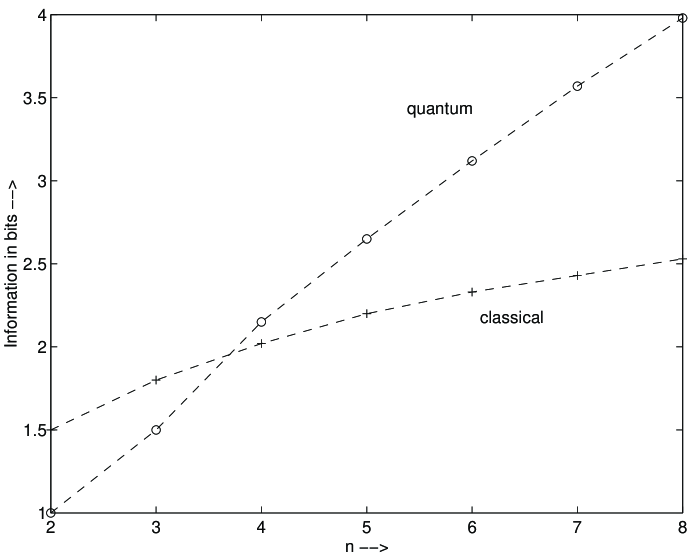
Figure 3: Classical vs. quantum information for small $n$

Since, the class membership is based on the combinations of the different partitions of $n$, rather than the combinations of $n$ directly as in the binomial distribution, the discrepancy between the actual information value and its upper bound is much less in the quantum case as compared to the classical case.

4 Discussion

The analysis done in this paper shows that a quantum measurement gives information roughly

$$\sqrt{n}/\!\log n$$ (11)

times that provided by the corresponding classical measurement, as shown in Figure 3.

As $n$ becomes large, the advantage over classical measurement becomes enormous. Put differently, for the same performance, one would need of the order of $2^{\sqrt{n}}$ classical elements where only $n$ quantum elements would suffice. This exponential advantage is what makes quantum algorithms for solving problems faster than the corresponding classical algorithms. This is also the explanation for why, from a computational point of view, quantum interactions are so fundamentally different from classical interactions.

This paper has considered the nature of the measurement process from the point of view of intrinsic information. Another perspective is to study situations which depart from classical logic; these include the Aharonov-Bohm, the EPR, and the Hansbury Brown-Twiss effects[13]. A setting for detection of objects without any interactions with the object was presented by Elitzur and Vaidman[2] with the Mach-Zehnder particle interferometer as the measurement apparatus. When both paths are clear, the particles are registered in one detector only. But if one of the paths is blocked then there is a fifty percent chance that the other detector will receive the particle. If this happens, then clearly one has determined the blockage of the path without having interacted with the object of the blockage. Using the notion of distributed measurement[9], the percentage for detecting without interaction can be further increased. If the photons are transmitted over two paths rather than one, we increase the variables that can be changed.

The research reported in this paper suggests several new investigations. One may wish to examine apparatus which is distributed in more than one spatial dimension and study the use of entangled states as well as that of coupled EPR particles.

References

- [1] G.S. Agarwal and S.P. Tewari, “An all-optical realization of the quantum Zeno effect.” Phys. Lett. A 185, 139-142 (1994).
- [2] A.C. Elitzur and L. Vaidman, “Quantum mechanical interaction free measurements.” Foundations of Physics 23, 987-997 (1993).
- [3] S.C. Kak, “On quantum numbers and uncertainty.” Nuovo Cimento 33B, 530-534 (1976).
- [4] S.C. Kak, “On information associated with an object.” Proc. of the Indian National Science Academy 50, 386-396 (1984).
- [5] S.C. Kak, “Quantum neural computing.” Advances in Imaging and Electron Physics, 94, 259-313 (1995).
- [6] S.C. Kak, “Information, physics, and computation.” Foundations of Physics 26, 127-137 (1996).
- [7] S.C. Kak, “Speed of computation and simulation.” Foundations of Physics 26, 1375-1386 (1996).
- [8] S.C. Kak, “The three languages of the brain.” In Learning as Self-Organization, K. Pribram and J. King (eds.). (Lawrence Erlbaum Associates, Mahwah, 1996, pages 185-219).
- [9] P.G. Kwiat, H. Weinfurter, T. Herzog, A. Zeilinger, and M.A. Kasevich, “Interaction-free measurements.” Physical Review Letters 74, 4763-4766 (1995).
- [10] H. Loo-Keng, Introduction to Number Theory. (Springer-Verlag, Berlin, 1982).
- [11] B. Misra and E.C.G. Sudarshan, “The Zeno’s paradox in quantum theory.” J. Math. Phys. 18, 756-763 (1977).
- [12] A. Peres, “Zeno paradox in quantum theory.” Am. J. Phys. 48, 931-932 (1980).
- [13] M.P. Silverman, More than One Mystery. (Springer-Verlag, New York, 1995).