Simulating the Effect of Decoherence and Inaccuracies on a Quantum Computer

Abstract

A Quantum Computer is a new type of computer which can solve problems such as factoring and database search very efficiently. The usefulness of a quantum computer is limited by the effect of two different types of errors, decoherence and inaccuracies. In this paper we show the results of simulations of a quantum computer which consider both decoherence and inaccuracies. We simulate circuits which factor the numbers 15, 21, 35, and 57 as well as circuits which use database search to solve the circuit satisfaction problem. Our simulations show that the error rate per gate is on the order of $10^{-6}$ for a trapped ion quantum computer whose noise is kept below $\pi/4096$ per gate and with a decoherence rate of $10^{-6}$. This is an important bound because previous studies have shown that a quantum computer can factor more efficiently than a classical computer if the error rate is of order $10^{-6}$.

Keywords:

Quantum Simulation, Ion Trap, Factoring, Database Search

1 Introduction

A quantum computer consists of atomic particles which obey the laws of quantum mechanics [TuHo95][Lloy95]. The complexity of a quantum system is exponential with respect to the number of particles. Performing computation using these quantum particles results in an exponential amount of calculation in a polynomial amount of space and time [Feyn85][Deut85]. This quantum parallelism is only applicable in a limited domain. Prime factorization is one such problem which can make effective use of quantum parallelism[Shor94]. This is an important problem because the security of the RSA public-key cryptosystem relies on the fact that prime factorization is computationally difficult[RiSA78].

Errors limit the effectiveness of any physical realization of a quantum computer. A quantum computer is subject to two different types of errors, decoherence and inaccuracies. Decoherence occurs when a quantum computer interacts with the environment. This interaction destroys the quantum parallelism by turning a quantum calculation into a classical one. The other type of error, inaccuracies in the implementation of gate operations, accumulates over time and destroys the results of the calculation.

In this paper we show results of simulations of a quantum computer which is subject to both decoherence and inaccuracies. These simulations assume the trapped ion model of a quantum computer proposed by Cirac and Zoller[CiZo95]. We study Shor’s factorization algorithm by simulating circuits which factor the numbers 15, 21, 35, and 57[Shor94]. We also simulate Grover’s database search algorithm with a circuit which solves the circuit satisfaction problem[Grov96]. The rest of this section gives a brief overview of quantum computers.

1.1 Qubits and Quantum Superposition

The basic unit of storage in a Quantum Computer is the qubit. A qubit is like a classical bit in that it can be in two states, zero or one. The qubit differs from the classical bit in that, because of the properties of quantum mechanics, it can be in both these states simultaneously[FeLS65]. A qubit which contains both the zero and one values is said to be in the superposition of the zero and one states. The superposition state persists until we perform an external measurement. This measurement operation forces the state to one of the two values. Because the measurement determines without doubt the value of the qubit, we must describe the possible states which exist before the measurement in terms of their probability of occurrence. These qubit probabilities must always sum to one because they represent all possible values for the qubit.

The quantum simulator represents the qubits of the computer using a complex vector space. Each state in the vector represents one of the possible values for the qubits. The bit values of a state are encoded as the index of that state in the vector. The simulator represents each encoded bit string with a non zero amplitude in the state vector. The probability of each state is defined as the square of this complex amplitude[FeLS65]. For a register with $M$ qubits, the simulator uses a vector space of dimension $2^{M}$.

1.2 Quantum Transformations and Logic Gates

A quantum computation is a sequence of transformations performed on the qubits contained in quantum registers[Feyn85][BaBe95]. A transformation takes an input quantum state and produces a modified output quantum state. Typically we define transformations at the gate level, i.e. transformations which perform logic functions. The simulator performs each transformation by multiplying the $2^{M}$ dimensional vector by a $2^{M}\times 2^{M}$ transformation matrix.

The basic gate used in quantum computation is the controlled-not, i.e. exclusive or gate. The controlled-not gate is a two bit operation between a control bit and a resultant bit. The operation of the gate leaves the control bit unchanged, but conditionally flips the resultant bit based on the value of the control bit.

1.3 The Ion Trap Quantum Computer

The ion trap quantum computer as proposed by Cirac and Zoller is one of the most promising schemes for the experimental realization of a quantum computer [CiZo95]. Several experiments have demonstrated simple quantum gates [MoMe95] [WiMM96]. Laser pulses directed at the ions in the trap cause transformations to their internal state. A common phonon vibration mode is used to communicate between the ions in the trap. A controlled-not gate is a sequence of laser pulses. We use the ion trap quantum computer as the model for our quantum simulator.

1.3.1 Qubits in the Ion Trap Quantum Computer.

Qubits are represented using the internal energy states of the ions in the trap. The ion trap represents a logic zero with the ground state of an ion, and a logic one with a higher energy state. The ion trap quantum computer also requires a third state which it uses to implement the controlled-not gate. In this paper we use a simplified model which, instead of using a third state for each qubit, uses a single third state which is shared amongst all the qubits. This simplified model reduces the simulation complexity exponentially without an appreciable loss of accuracy[ObDe97a].

1.3.2 Transformations in the Ion Trap.

An operation in the ion trap quantum computer is a sequence of laser pulses. Each laser pulse is defined by one of the transformation matrices shown in equation 1. $\theta$ corresponds to the duration of the laser pulse and $\phi$ corresponds to the phase. A two bit controlled-not gate is a sequence of five laser pulses, two V and three U transformations. A single bit not gate can be implemented with three laser pulses and the three bit controlled-controlled-not gate requires seven laser pulses.

$$U=\left[\begin{array}[]{cccc}1&0&0&0\\ 0&\cos\frac{\theta}{2}&-ie^{-i\phi}\sin\frac{\theta}{2}&0\\ 0&-ie^{i\phi}\sin\frac{\theta}{2}&\cos\frac{\theta}{2}&0\\ 0&0&0&1\end{array}\right]V=\left[\begin{array}[]{cc}\cos\frac{\theta}{2}&-ie^{-i\phi}\sin\frac{\theta}{2}\\ -ie^{i\phi}\sin\frac{\theta}{2}&\cos\frac{\theta}{2}\\ \end{array}\right]$$ (1)

2 Simulating a Quantum Computer

Our quantum computer simulator simulates circuits at the gate level. The simulator implements one, two and three bit controlled-not gates as well as rotation gates. The simulator implements each gate as a sequence of laser pulses, and represents the entire vector space throughout the simulation.

2.1 Operational Errors and Decoherence

The simulator models inaccuracies by adding a small deviation to the two angles of rotation $\theta$ and $\phi$. Each operational error angle is drawn from a gaussian distribution with a parametrized mean ($\mu$) and standard deviation ($\sigma$). Errors with non zero $\mu$, called mean errors, correspond to systematic calibration errors, and errors with non zero $\sigma$, referred to as standard deviation errors, correspond to noise in the laser apparatus.

Because the phonon mode is coupled to all the qubits in the computer, it is the largest source of decoherence[MoMe95]. For this reason we only model the phonon decoherence and not the decoherence of the individual qubits.

We model the decoherence of the phonon mode by performing an additional operation after each laser pulse. Equation 2 shows this transformation which has the effect of decaying the amplitude of the states in the phonon state. This decay transformation is based on the quantum jump approach[Carm93]. The decay parameter (dec) remains constant throughout the entire simulation.

$$\begin{array}[]{lcr}\begin{array}[]{c}|\psi>|0>_{p}\\ |\psi>|1>_{p}\end{array}&\Rightarrow&\begin{array}[]{r}|\psi>|0>_{p}\\ e^{-dec/2}|\psi>|1>_{p}\end{array}\end{array}$$ (2)

This method of modeling decoherence implicitly models spontaneous emission. Because the state is never renormalized, the total norm at each step represents the probability that the calculation survives up to that point without a spontaneous emission occurring. An alternative method for modeling decoherence is to renormalize the state at each step and then, based on a probability of emission, cause emissions at different points in the calculation. This method has the disadvantage that, because we cause emissions at random points in the calculation, we must run multiple simulations each with different initial random seeds to average out any bias caused by the random number generator. We have shown however that both methods for modeling decoherence give essentially the same results[ObDe97a].

Because the simulator applies the decoherence transformation once per laser pulse, the parameter dec has units of (decoherence/laser pulse). To convert these units to decoherence per unit time we must consider the switching time of the laser. The $dec$ parameter is simply the switching speed divided by the decoherence time. Recent experiments show switching speeds of 20kHz for a controlled-not gate, i.e. four $\pi$ pulses, and a decoherence rate of a few kHz[MoMe95]. This corresponds to a decoherence parameter value between $10^{-2}$ and $10^{-3}$.

2.2 Quantum Circuits

Much of the current interest in quantum computation is due to the discovery of an efficient algorithm by Peter Shor to factor numbers[Shor94]. By putting the qubit register $A$ in the superposition of all values and calculating the function $f(A)=X^{A}modN$, a quantum computer calculates all the values of $f(A)$ simultaneously. Where $N$ is the number to be factored, and $X$ is a randomly selected number which is relatively prime to $N$. The quantum factoring circuit also contains operations to create the superposition state at the beginning of the circuit, and extract the period at the end of the circuit. The circuit to calculate $f(A)$ can be performed in $O(L^{3})$ time using repeated squaring[Desp96], i.e. a sequence of multiplications performed modulo $N$.

Grover’s database search algorithm searches for a key, from a set of matching keys, in an unsorted database[Grov96]. The keys are defined by a function which can be evaluated in unit time. After evaluating this function a diffusion transformation is performed which amplifies the probability in the states with matching keys. Grover shows that after performing $O(\sqrt{(}N))$ evaluation steps and diffusion transformations the probability of measuring a matching key is greater than 1/2.

3 Simulation Results

In this section we study how decoherence and operational errors degrade the fidelity of the factoring and database search algorithms.

The fidelity, as defined by $fidelity=\|<\varphi|\psi>\|^{2}$, measures how close a state with error in it is to the correct result. The fidelity is defined as the inner product between the simulation with errors ($\psi$) and the correct result ($\varphi$).

Table 1 shows all the benchmarks used in our simulation studies. To show the complexity of simulating these benchmarks we show the simulation time for each. This time assumes a single 300 MHz processor and the simulations include only operational error. All the factoring benchmarks were run using a parallel version of the simulator[ObDe98]. We have run simulations on as many as 256 processors, and the simulator achieves near linear speedup.

Table 1: Benchmarks used in simulation studies

	Number of	Number of		Simulation
Benchmark	qubits	laser pulses	Description	time (secs)
			Circuit SAT using the Grover
grover	13	1,838	database search algorithm	10
			One modulo multiply step
mult	16	8,854	from the factor-15 problem	282
			Factor-15 problem using
factor15	18	70,793	3 qubits for A	10,465
			Factor-21 problem using
factor21	24	69,884	6 qubits for A	272,276
			Factor-35 problem using
factor35	27	99,387	6 qubits for A	3,083,520
			Factor-57 problem using
factor57	27	97,939	6 qubits for A	3,067,853

Because of round off error, in the factoring algorithm, the choice of the number of bits to use in the $A$ register affects the probability seen after performing the FFT[Shor94]. Shor suggest using $2L+1$ bits for an $L$ bit factorization, but for the numbers used in our studies we can use less. For the factor15 problem the period is a power of two, i.e. four, and therefore there is no round off error. For the numbers 21, 35 and 57, the probability given by the FFT does not increase for more than six bits. Also we are mainly concerned with observing the fidelity for these circuits, and the fidelity is always calculated before the FFT.

3.1 Operational Errors

In this section we consider operational errors without any decoherence. We first investigate the significance of errors in the angle $\phi$, by varying the amount of error in the angles $\theta$ and $\phi$ separately. In all other simulations we vary the angles $\theta$ and $\phi$ together.

To average the random bias out of simulations with non zero $\sigma$ we run multiple simulations each with different initial random seeds. To get a single simulation point we run at least four simulations, and in many cases we run more to establish upper and lower confidence intervals for the average of the ending fidelities[HiMo80]. For simulations which include errors in the angle $\theta$ we run enough simulations so that the average of the fidelities is within 0.02 of the actual mean of the distribution with an upper and lower confidence of 95%. There is more variability in the fidelity for simulations which consider only $\phi$ errors, so for these we obtain the 95% confidence intervals to within 0.03 of the mean.

3.1.1 Significance of Errors in the Angle $\phi$.

Fig. 1 shows how operational errors degrade the fidelity for the factor15 benchmark. In Fig. 1(a) we vary the mean and standard deviation and introduce both $\theta$ and $\phi$ errors. In Fig. 1(b) we only introduce $\theta$ errors. Comparing the two graphs shows that the combination of $\theta$ and $\phi$ errors produces a lower fidelity than $\theta$ errors alone.

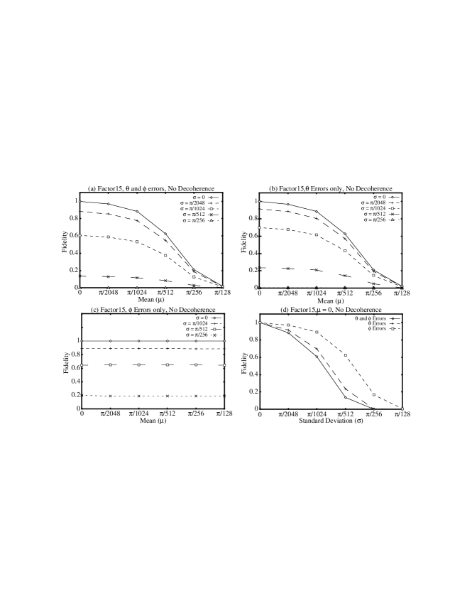
Figure 1: Inaccuracies for factor15 (a) $\theta$ and $\phi$ errors (b) $\theta$ errors (c) $\phi$ errors (d) $\theta$ and $\phi$ errors, $\theta$ errors, $\phi$ errors

Fig. 1(c) shows the effect of only $\phi$ errors. As the graph shows noise degrades the fidelity, but adding a constant amount of error has no effect. Fixed magnitude $\phi$ errors have no effect because the laser transformations are always performed in pairs, and an error in the second transformation cancels an error in the first transformation. In Fig. 1(d) we compare the effect of $\theta$ and $\phi$ errors alone and their combined effect. The highest degradation occurs when considering both $\theta$ and $\phi$ errors, and $\theta$ errors produce a more significant effect than $\phi$ errors.

3.1.2 Operational Errors for the Grover Benchmark.

Fig. 2 shows mean and standard deviation operational errors for the grover benchmark. The figures show the probability of finding a correct key for twelve iterations of the algorithm. When running the database search it is important to stop after the correct iteration, because the probability decreases if we run too many iterations[BoBr96]. For our case the highest probability occurs after the eighth iteration.

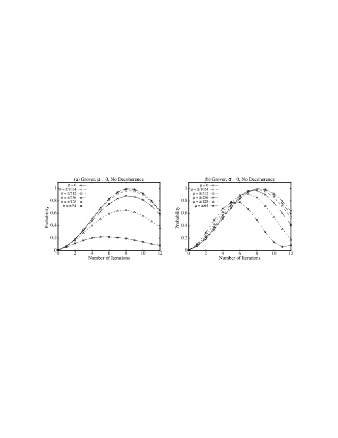
Figure 2: Inaccuracies for the grover benchmark. (a) $\sigma$ Errors. (b) $\mu$ errors

Fig. 2(a) shows that the peak probability is above 0.5 for $\sigma$ errors as great as $\pi/128$, and for an error rate of $\pi/64$ the peak probability is 0.2. Also for $\sigma$ errors the peak probability occurs after the same iteration for all errors less than $\pi/128$. However $\mu$ errors, as shown in Fig. 2(b), shift the peak so that it occurs at an earlier iteration. The peaks are higher for $\mu$ errors than they are for $\sigma$ errors with the same level of error. However, since we can only perform a single measurement, the shift in the peak values causes a further reduction in the probability if we measure after the eighth iteration.

3.1.3 Fidelity at Intermediate Points for the Factoring Benchmarks.

Fig. 3 shows the fidelity at intermediate points in the calculation for the factor21, and factor57 benchmarks.

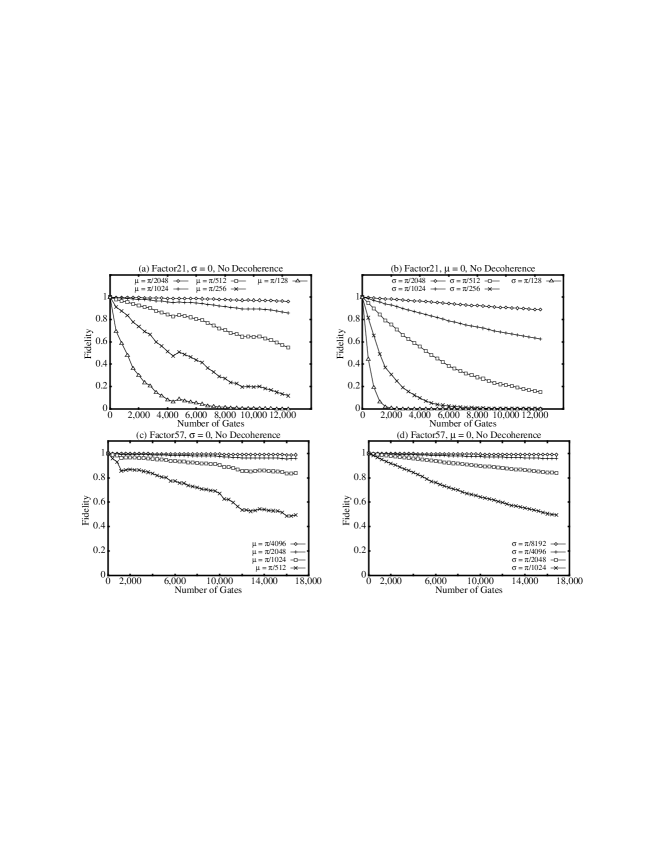
Figure 3: Fidelity as a function of the number of gates for factor21 and factor57

Standard deviation errors produce a more significant effect than $\mu$ errors of the same magnitude. This is due to a cancellation effect for mean errors which is very similar to the cancellation effect exhibited by $\phi$ errors[ObDe97a]. This cancellation effect occurs because of the nature of reversible computation and causes the fidelity to go through periods where it increases. Because we perform operations in pairs, where the two operations are inverses of each other, an error in one operation may reverse the error from an earlier operation. Standard deviation errors also exhibit this effect but it is reduced because we average the results from multiple simulations.

3.2 Decoherence Errors

Fig. 4 shows how the fidelity of a computation decreases over time in the presence of decoherence. Fig. 4 shows the fidelity at intermediate points in the calculation for the four factoring benchmarks. For small amounts of decoherence, i.e. $10^{-6}$ or less, the fidelity is not adversely affected. A decoherence rate of $10^{-4}$ results in a steady decrease in the fidelity over the course of the computation, and for rates even higher the fidelity drops off very quickly. As the figure shows, decoherence has a similar effect on all of the benchmarks.

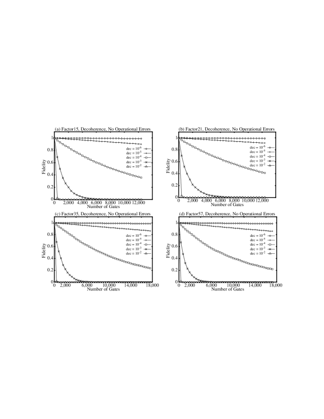
Figure 4: Fidelity as a function of the number of gates for decoherence in the factor15, factor21, factor35 and factor57 benchmarks

3.3 The Correlation Between Decoherence and Operational Errors

Both decoherence and operational error cause a degradation of the fidelity in a quantum computation. Decoherence degrades the fidelity through the decay of the phonon state, and operational errors result in the accumulation of amplitude in unwanted states. The combined effect of these two factors is a degradation which is worse than either factor considered alone. We can represent the combined effect as: $F_{dec,op}=F_{dec}\bullet F_{op}+\Omega(F_{dec},F_{op})$ Where $F_{dec}$ and $F_{op}$ are the fidelities of simulations for decoherence and operational error considered separately, and $\Omega(F_{dec},F_{op})$ is the correlation between the two types of error. As Table 2 shows the correlation is very low. We calculated the correlation by running simulations which considered decoherence and operational error together. For all the benchmarks the maximum correlation is at most $1.14\times 10^{-2}$. This result means that we can simulate decoherence and operational errors separately, and combine the results to obtain their collective effect on a calculation.

Table 2: Correlation ($\Omega$) between decoherence and operational errors

Benchmark and Simulation Model	Maximum $\Omega$	Average $\Omega$
mult, $\mu$=0, $\sigma$ = $\pi/1024$ - $\pi/64$	$5.76\times 10^{-5}$	$3.63\times 10^{-6}$
mult, $\sigma$ = 0, $\mu$ = $\pi/1024$ - $\pi/64$	$9.26\times 10^{-3}$	$5.51\times 10^{-4}$
factor15, $\sigma$ = $\pi/1024$, $\mu$ = 0	$4.15\times 10^{-3}$	$3.96\times 10^{-4}$
factor15, $\sigma$ = 0, $\mu$ = $\pi/1024$	$1.14\times 10^{-2}$	$8.76\times 10^{-4}$
grover, $\mu$=0, $\sigma$ = $\pi/1024$ - $\pi/128$	$1.78\times 10^{-3}$	$1.02\times 10^{-4}$
grover, $\sigma$=0, $\mu$ = $\pi/1024$ - $\pi/128$	$2.67\times 10^{-3}$	$2.36\times 10^{-4}$

The complexity of simulating decoherence alone is much lower than the complexity of simulating operational errors. This is because the decay transformation does not have any off diagonal terms, and therefore it does not introduce any new error states. The simulator only needs to represent enough states to represent the superposition state. Instead of using the index of a state to represent its bit value, the simulator now keeps an extra field for each state which holds the current value of the bit string for that state.

Using this new method for modeling decoherence, the simulator only needs to allocate $O(2^{L})$ states to simulate the factorization of an $L$ bit number. To represent all the qubits for this problem, the simulator would need to allocate $O(2^{4L})$ states. This reduces the memory requirements and simulation complexity by a factor of $O(2^{3L})$. For example the simulation of the factor15 circuit requires only 1/4096 the amount of time as before.

3.4 The Error Rate per Gate

As our simulation results show, a modest amount of error destroys even a relatively small calculation. If quantum computers are to be useful, we must be able to perform calculations which are even larger than the ones considered here. These larger calculations will therefore require the use of quantum error correcting codes[Stea96]. Several recent studies have shown that, by using fault tolerant techniques, if the error of an individual gate is low enough we can perform a useful quantum calculation of indefinite length[Pres96][KnLZ96]. This accuracy threshold is expressed in terms of the probability of error per gate. We can use the results of our simulation studies to show how this error probability relates to decoherence and inaccuracies.

Table 3 shows the error rate per gate considering decoherence and operational errors for the factor57 benchmark. Error rates for the other factoring benchmarks as well as error rates for the combination of decoherence and operational errors are given in [ObDe97b]. The error rate is calculated as (1 - Fidelity)/Number of Gates. To get the error rate for a particular amount of error, we calculate the error rate after every tenth gate in a computation and take the average. A gate is either a one, two or three bit controlled-not gate or a single bit rotation. It takes five laser pulses on average to implement each gate.

Table 3: Average error rate per gate for the factor57 benchmark

Decoherence		Operational Errors, $\mu=0$		Operational Errors, $\sigma=0$
dec	Error Rate	$\sigma$	Error Rate	$\mu$	Error Rate
$10^{-7}$	$9.1\times 10^{-8}$	$\pi/8192$	$6.6\times 10^{-7}$	$\pi/4096$	$7.9\times 10^{-7}$
$10^{-6}$	$9.1\times 10^{-7}$	$\pi/4096$	$2.6\times 10^{-6}$	$\pi/2048$	$3.1\times 10^{-6}$
$10^{-5}$	$8.8\times 10^{-6}$	$\pi/2048$	$1.0\times 10^{-5}$	$\pi/1024$	$1.2\times 10^{-5}$
$10^{-4}$	$6.5\times 10^{-5}$	$\pi/1024$	$3.6\times 10^{-5}$	$\pi/512$	$4.4\times 10^{-5}$

To perform a computation of arbitrary length the error rate must be about $10^{-5}$ for one and two bit gates and $10^{-3}$ for three bit gates[Pres96]. An error rate of $10^{-5}$ corresponds to operational errors with $\sigma=\pi/2048$ and decoherence of $10^{-5}$. Table 3 shows that we can tolerate an even higher level of constant magnitude errors. The error rate is $10^{-5}$ for operational errors with $\mu=\pi/1024$.

To perform a quantum factorization which is more efficient than a classical one the error threshold is even tighter, roughly $10^{-6}$. This corresponds to operational errors with $\sigma<\pi/4096$ and a decoherence rate of $10^{-6}$.

Using the error rate of our factoring circuits to predict the error rate for error correction circuits assumes that these two types of circuits behave in a similar manner. These circuits are similar because they are both built from the same types of elementary gates, i.e. controlled-not gates. Also the error rate, for a given amount of error, is very similar for all the factoring circuits that we considered. Lastly effects that we have seen such as error cancellation are a by-product of the fact that quantum circuits and gates are implemented in a reversible fashion. Because of the nature quantum mechanics quantum circuits will always be implemented in this way.

4 Conclusion

Quantum computation is a new type of computation which can achieve exponential parallelism. The feasibility of a quantum computer is threatened by two types of errors, decoherence and inaccuracies. In this paper we performed simulations of a quantum computer running Shor’s factoring algorithm and Grover’s database search algorithm to access the feasibility of implementing a quantum computer.

Our simulations show that random inaccuracies (noise) are more significant than fixed magnitude inaccuracies for the ion trap quantum computer. Also errors in the duration of the laser pulse are more significant than errors in the phase of the laser. For the problems considered in this paper we show that noise or constant magnitude inaccuracies of magnitude $\pi/512$ or greater cause a significant impact on the fidelity of the calculation.

Our simulations also show that a quantum computation can tolerate a decoherence rate as high as $10^{-5}$. For the ion trap computer this corresponds roughly to a decoherence lifetime of 50 milliseconds and a switching speed of 500 nanoseconds. We also show that inaccuracies and decoherence are uncorrelated and can be simulated separately.

Our simulations relate the physical quantities of inaccuracies and decoherence to the probability of error per gate. An error rate per gate on the order of $10^{-6}$ corresponds to inaccuracies of less than $\pi/4096$ per laser operation and a decoherence rate of $10^{-6}$. A quantum computer with this error rate, if it uses quantum error correcting codes, could factor a number more efficiently than a classical computer. This assumes that the quantum circuits used to implement factoring with error correction codes behave in the same manner as the factoring circuits used in this paper.

Acknowledgments

The authors are members of the Quantum Information and Computation (QUIC) consortium. We wish to thank our QUIC colleagues: Jeff Kimble, John Preskill, Hideo Mabuchi and Dave Vernooy. This work is supported in part by ARPA under contract number DAAH04-96-1-0386.

References

- [BaBe95] A. Barenco et al. “Elementary Gates for Quantum Computation.” Phys. R. A 52, 3457-3467. 1995.
- [BoBr96] M. Boyer et al. “Tight bounds on quantum searching.” Proc. PhysComp96.
- [Carm93] H.J. Carmichael. An Open Systems Approach to Quantum Optics, Lecture notes in Physics, (Springer, Berlin). 1993.
- [CiZo95] J.I. Cirac, and P. Zoller. “Quantum Computations with Cold Trapped Ions.” Phys. Rev. Lett. 74, Number 20. May 15, 1995.
- [Desp96] A. Despain. “Quantum Networks” in Quantum Computing. JASON Report JSR-95-115. pp 49-81. The MITRE Corp. 1996.
- [Deut85] D. Deutsch. “Quantum Theory, the Church-Turing Principle and the Universal Quantum Computer.” Proc. R. Soc. Lond. A 400, pp 97-117. 1985.
- [FeLS65] R. Feynman, R. Leighton, and M. Sands. The Feynman Lectures on Physics III. Addison-Wesley Publishing Company. 1965.
- [Feyn85] R. Feynman. “Quantum Mechanical Computers.” Found. of Phys., 16, 1985.
- [Grov96] L. Grover. “A Fast Quantum Mechanical Algorithm for Database Search.” Proc., STOC 1996.
- [HiMo80] W. W. Hines, D. C. Montgomery. Probability and Statistics in Engineering and Management Science. John Wiley & Sons, Inc. 1980.
- [KnLZ96] E. Knill et al. “Accuracy Threshold for Quantum Computation.” 1996.
- [Lloy95] S. Lloyd. “Quantum-Mechanical Computers.” Scientific American. Vol. 273, No. 4, pp 140-145. October 1995.
- [MoMe95] C. Monroe et al. “Demonstration of a Universal Quantum Logic Gate.” Phys. Rev. Lett. 75, 4714. Dec. 1995.
- [ObDe97a] K. Obenland, and A. Despain. “Models to Reduce the Complexity of Simulating a Quantum Computer.” ISI Tech. Report. November 1997.
- [ObDe97b] K. Obenland, and A. Despain. “Simulating the Effect of Decoherence and Inaccuracies on a Quantum Computer.” ISI Tech. Report. December 1997.
- [ObDe98] K. Obenland, and A. Despain. “A Parallel Quantum Computer Simulator.” High Performance Computing 1998.
- [Pres96] J. Preskill. “Reliable Quantum Computers.” Proc. R. Soc. Lond. A. 1996.
- [RiSA78] R.L. Rivest et al. “A Method for Obtaining Digital Signatures and Public-Key Cryptosystems.” Comm. ACM. 21, p 120. 1978.
- [Shor94] P. Shor. “Algorithms for Quantum Computation: Discrete Logarithms and Factoring.” Proc., 35th Annual FOCS pp. 124-134. November 1994.
- [Stea96] A.M. Steane. “Multiple Particle Interference and Quantum Error Correction.” Proc. R. Soc. Lond. A 452, 2551. 1996.
- [TuHo95] Q.A. Turchette et al. “Measurement of Conditional Phase Shifts for Quantum Logic.” Phys. Rev. Lett. 75, 4710. Dec. 1995.
- [WiMM96] D. Wineland et al. “Quantum State manipulation of Trapped Atomic Ions.” Proc. R. Soc. Lond. A. December 1996.