Some Notes on Parallel Quantum Computation

Abstract

We exhibit some simple gadgets useful in designing shallow parallel circuits for quantum algorithms. We prove that any quantum circuit composed entirely of controlled-not gates or of diagonal gates can be parallelized to logarithmic depth, while circuits composed of both cannot. Finally, while we note the Quantum Fourier Transform can be parallelized to linear depth, we exhibit a simple quantum circuit related to it that we believe cannot be parallelized to less than linear depth, and therefore might be used to prove that ${\bf QNC}<{\bf QP}$.

Much of computational complexity theory has focused on the question of what problems can be solved in polynomial time. Shor’s quantum factoring algorithm [8] suggests that quantum computers might be more powerful than classical computers in this regard, i.e. that ${\bf QBP}$ might be a larger class than ${\bf P}$, or rather ${\bf BP}$, the class of problems solvable in polynomial time by a classical probabilistic Turing machine with bounded error.

More recently, a distinction has been made between ${\bf P}$ and the class ${\bf NC}$ of efficient parallel computation, namely the subset of ${\bf P}$ of problems which can be solved by a parallel computer with a polynomial number of processors in polylogarithmic time, i.e. ${\cal O}(\log^{k}n)$ time for some $k$, where $n$ is the number of bits of the input [7]. Equivalently, ${\bf NC}$ problems are those solvable by Boolean circuits with a polynomial number of gates and polylogarithmic depth.

This distinction seems especially relevant for quantum computers, where decoherence makes it difficult to do more than a limited number of computation steps reliably. Since decoherence due to storage errors is essentially a function of time, we can avoid it by doing as many of our quantum operations at once as possible; if we can parallelize our computation to logarithmic depth, we can solve exponentially larger problems. (Gate errors, on the other hand, will not be improved by parallelization, and may even get worse if the parallel algorithm involves more gates.)

We define quantum operators and quantum circuits as follows:

Definition 0.1.

A quantum operator on $n$ qubits is a unitary rank-$2n$ tensor $U$ where $U_{a_{1}a_{2}\ldots a_{n}}^{b_{1}b_{2}\ldots b_{n}}$ is the amplitude of the incoming and outgoing truth values being $a_{1},a_{2},\ldots a_{n}$ and $b_{1},b_{2},\ldots b_{n}$ respectively, with $a_{i},b_{i}\in\{0,1\}$ for all $i$. However, we will usually write $U$ as a $2^{n}\times 2^{n}$ unitary matrix $U_{ab}$ where $a$ and $b$’s binary representations are $a_{1}a_{2}\cdots a_{n}$ and $b_{1}b_{2}\cdots b_{n}$ respectively.

A one-layer circuit consists of the tensor product of one- and two-qubit gates, i.e. rank 2 and 4 tensors, or $2\times 2$ and $4\times 4$ unitary matrices. This is an operator that can be carried out by a set of simultaneous one-qubit and two-qubit gates, where each qubit interacts with at most one gate.

A quantum circuit of depth $k$ is a quantum operator written as the product of $k$ one-layer circuits. The depth of a quantum operator is the depth of the shallowest circuit equal to it.

Here we are allowing arbitrary two-qubit gates. If we like, we can restrict this to controlled-$U$ gates, of the form $\left(\!\begin{array}[]{cccc}1&0&0&0\\ 0&1&0&0\\ 0&0&u_{11}&u_{12}\\ 0&0&u_{21}&u_{22}\end{array}\!\right)$, or more stringently to the controlled-not gate $\left(\!\begin{array}[]{cccc}1&0&0&0\\ 0&1&0&0\\ 0&0&0&1\\ 0&0&1&0\end{array}\!\right)$. For these, we will call the first and second qubits the input and target qubit respectively, even though they don’t really leave the input qubit unchanged, since they entangle it with the target.

Since either of these can be combined with one-qubit gates to simulate arbitrary two-qubit gates [1], these restrictions would just multiply our definition of depth by a constant. The same is true if we wish to allow gates that couple $k>2$ qubits as long as $k$ is fixed, since any $k$-qubit gate can be simulated by some constant number of two-qubit gates.

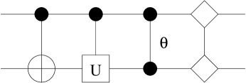
Fig. 1.: Our notation for controlled-not, controlled-$U$, symmetric phase shift, and arbitrary diagonal gates.

In order to design a shallow parallel circuit for a given quantum operator, we want to be able to use additional qubits or “ancillae” for intermediate steps in the computation, equivalent to additional processors in a parallel quantum computer. However, to avoid entanglement, we demand that our ancillae start and end in a pure state $|0\rangle$, so that the desired operator appears as the diagonal block of the operator performed by the circuit on the subspace where the ancillae are zero.

Then in analogy with ${\bf NC}$ we propose the following definition:

Definition 0.2.

Let $F$ be a family of quantum operators, i.e. $F(n)$ is a $2^{n}\times 2^{n}$ unitary matrix on $n$ qubits. We say that $F(n)$ is embedded in an operator $M$ with $m$ ancillae if $M$ is a $2^{m+n}\times 2^{m+n}$ matrix which preserves the subspace where the ancillae are set to $|0\rangle$, and if $M$ is identical to $F(n)\otimes\bf{1}^{2^{m}}$ when restricted to this subspace.

Then $F$ is in ${\bf QNC}^{k}$ if, for some constants $c_{1}$, $c_{2}$ and $j$, $F(n)$ can be embedded in a circuit of depth at most $c_{1}\log^{k}n$, with at most $c_{2}n^{j}$ ancillae. Then ${\bf QNC}=\cup_{k}{\bf QNC}^{k}$, the set of operators parallelizable to polylogarithmic depth with a polynomial number of ancillae.

To extend this definition from quantum operators to decision problems in the classical sense, we have to choose a measurement protocol, and to what extent we want errors bounded. We will not explore those issues here.

We will use the notation in figure 1 for our various gates: the controlled-not and controlled-$U$, the symmetric phase shift $\left(\!\begin{array}[]{cccc}1&0&0&0\\ 0&1&0&0\\ 0&0&1&0\\ 0&0&0&e^{i\theta}\end{array}\!\right)$, and arbitrary diagonal gates $\left(\!\begin{array}[]{cccc}e^{i\theta_{00}}&0&0&0\\ 0&e^{i\theta_{01}}&0&0\\ 0&0&e^{i\theta_{10}}&0\\ 0&0&0&e^{i\theta_{11}}\end{array}\!\right)$.

1 Permutations

In classical circuits, one can move wires around as much as one likes. In a quantum computer, it may be more difficult to move a qubit from place to place. However, we can easily show that we can do arbitrary permutations in constant depth:

Proposition 1.3.

Any permutation of $n$ qubits can be performed in 4 layers of controlled-not gates with $n$ ancillae, or in 6 layers with no ancillae.

Fig. 2.: Permuting $n$ qubits in $4$ layers using $n$ ancillae.

Proof 1.4.

The first part is obvious; simply copy the qubits into the ancillae, cancel the originals, recopy them from the ancillae in the desired order, and cancel the ancillae. This is shown in figure 2.

Fig. 3.: Any cycle, and therefore any permutation, is the composition of two sets of disjoint transpositions.

Fig. 4.: Switching two qubits with three controlled-nots.

Without ancillae, we can use the fact that any permutation can be written as the composition of two sets of disjoint transpositions [9]. To see this, first decompose it into a product of disjoint cycles, and then note that a cycle is the composition of two reflections, as shown in figure 3. Two qubits can be switched with 3 layers of controlled-not gates as shown in figure 4, so any permutation can be done in 6 layers. ∎

2 Fan-out

To make a shallow parallel circuit, it is often important to fan out one of the inputs into multiple copies. The controlled-not gate can be used to copy a qubit onto an ancilla in the pure state $|0\rangle$ by making a non-destructive measurement:

$$(\alpha|0\rangle+\beta|1\rangle)\otimes|0\rangle\,\to\,\alpha|00\rangle+\beta|11\rangle$$

Note that the final state is not a tensor product of two independent qubits; the two qubits are completely entangled. Making an unentangled copy requires non-unitary, and in fact non-linear, processes since

$$(\alpha|0\rangle+\beta|1\rangle)\otimes(\alpha|0\rangle+\beta|1\rangle)=\alpha^{2}|00\rangle+\alpha\beta(|01\rangle+|10\rangle)+\beta^{2}|11\rangle$$

has coefficients quadratic in $\alpha$ and $\beta$.

This means that disentangling or uncopying the ancillae by the end of the computation, returning them to their initial state $|0\rangle$, is a non-trivial and important part of a quantum circuit. There are, however, some special cases where this can be done easily.

Suppose we have a series of $n$ controlled-$U$ gates all with the same input qubit. Rather than applying them in series, we can fan out the input into $n$ copies by splitting it $\log_{2}n$ times, apply them to the target qubits, and uncopy them afterward, thus reducing the circuit’s depth to ${\cal O}(\log n)$ depth.

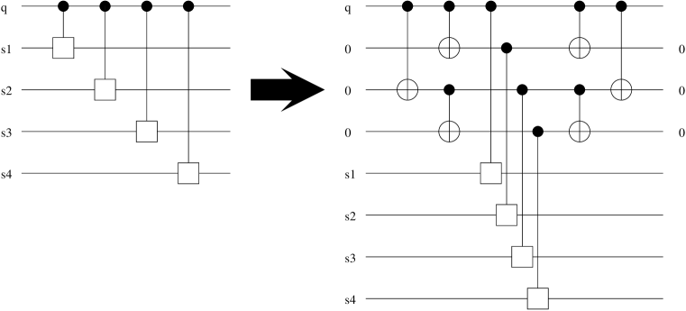
Fig. 5.: Parallelizing $n$ controlled gates on a single input qubit $q$ to ${\cal O}(\log n)$ depth.

Proposition 2.5.

A series of $n$ controlled gates coupling the same input to $n$ target qubits can be parallelized to ${\cal O}(\log n)$ depth with ${\cal O}(n)$ ancillae.

Proof 2.6.

The circuit in figure 5 copies the input onto $n-1$ ancillae, applies all the controlled gates simultaneously, and uncopies the ancillae back to their original state. Its total depth is $2\log_{2}n+1$. ∎

This kind of symmetric circuit, in which we uncopy the ancillae to return them to their original state, is similar to circuits designed by the Reversible Computation Group at MIT [4] for reversible classical computers.

3 Diagonal and mutually commuting gates

Fan-in seems more difficult in general. Classically, if a single qubit receives controlled gates from $n$ inputs, we can calculate the composition of these in ${\cal O}(\log n)$ time by composing them in pairs, but it is unclear when we can do this with unitary linear operators. One special case where it is possible is if all the gates are diagonal:

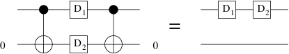
Fig. 6.: Using entanglement to parallelize diagonal operators.

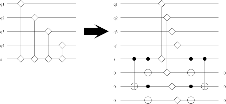
Fig. 7.: Parallelizing $n$ diagonal gates on a single qubit as in proposition 2.5.

Proposition 3.7.

A series of $n$ diagonal gates coupling the same qubit to $n$ others can be parallelized to ${\cal O}(\log n)$ depth with ${\cal O}(n)$ ancillae.

Proof 3.8.

Here the entanglement between two copies of a qubit becomes an asset. Since diagonal matrices don’t mix Boolean states with each other, we can act on a qubit and an entangled copy of it with two diagonal matrices $D_{1}$ and $D_{2}$ as in figure 6. When we uncopy the ancilla, we have the same effect as if we had applied both matrices to the original. Then the same kind of circuit as in proposition 2.5 works, as shown in figure 7. ∎

Since matrices commute if and only if they can be simultaneously diagonalized, we can generalize this to the case where a set of controlled-$U$ gates applied to a given target qubit have mutually commuting $U$s:

Proposition 3.9.

A series of of $n$ controlled-$U$ gates acting on a single qubit, where the $U$s mutually commute, can be parallelized to ${\cal O}(\log n)$ depth with ${\cal O}(n)$ ancillae.

Proof 3.10.

Since the $U$s all commute, they can all be diagonalized by the same unitary operator $T$. Apply $T$ to the target qubit, parallelize the circuit using proposition 3.7, and put the target qubit back in the original basis by applying $T^{-1}$. This is all done with a circuit of depth $2\log_{2}n+3$. ∎

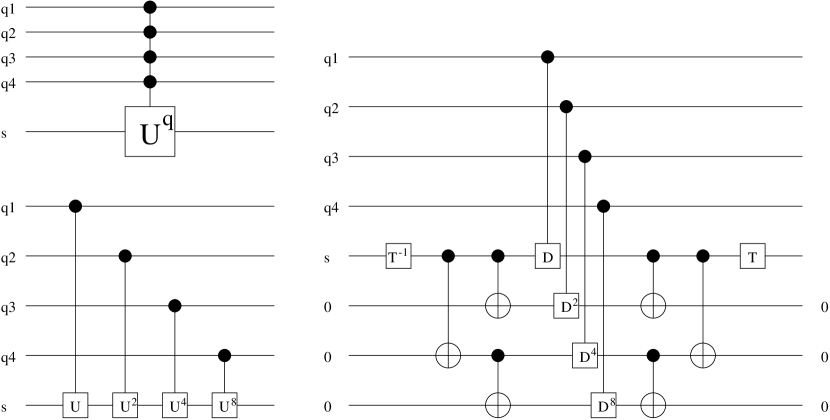
Fig. 8.: Applying an operator $U$ $q$ times, where $q$ is given in binary by the control qubits.

As an example, in figure 8 we show a circuit that applies the $q$th power of an operator $U$ to a target qubit, where $0\leq q<2^{k}$ is given by $k$ control qubits as a binary integer. We can do this because $U,U^{2},U^{4},\ldots$ can be simultaneously diagonalized, since $U^{q}=TD^{q}T^{-1}$. Note that this works for operators $U$ that act on any number of qubits.

We can extend this to circuits in general whose gates are mutually commuting, which includes diagonal gates:

Proposition 3.11.

Any circuit consisting of diagonal or mutually commuting gates, each of which couples at most $k$ qubits, can be parallelized to depth ${\cal O}(n^{k-1})$ with no ancillae, and to depth ${\cal O}(\log n)$ with ${\cal O}(n^{k})$ ancillae. Therefore, any family of such circuits is in ${\bf QNC}^{1}$.

Proof 3.12.

Since all the gates commute, we can sort them by which qubits they couple, and arrive at a compressed circuit with one gate for each $k$-tuple. This gives $\left(\!\begin{array}[]{c}n\\ k\end{array}\!\right)={\cal O}(n^{k})$ gates, but by performing groups of $n/k$ disjoint gates simultaneously we can do all of them in depth ${\cal O}(n^{k-1})$.

By making ${\cal O}(n^{k-1})$ copies of each qubit, we can then use propositions 3.7 and 3.9 to reduce this further to ${\cal O}(\log n)$ depth. ∎

This is hardly surprising; after all, diagonal gates are just conditional phase shifts, and saying that two gates commute is almost like saying that they can be performed simultaneously.

4 Circuits of controlled-not gates

We can also fan in controlled-not gates. Figure 9 shows how to implement $n$ controlled-not gates on the same target qubit in depth $2\log_{2}n+1$. The ancillae carry the intermediate “sums mod 2” of the inputs, and we add them in pairs.

Fig. 9.: Parallelizing $n$ controlled-not gates to ${\cal O}(\log n)$ depth by adding them in pairs.

We can use a generalization of this circuit to show that any circuit composed entirely of controlled-not gates can be parallelized to logarithmic depth:

Proposition 4.13.

Any circuit on $n$ qubits composed entirely of controlled-not gates can be parallelized to ${\cal O}(\log n)$ depth with ${\cal O}(n^{2})$ ancillae. Therefore, any family of such circuits is in ${\bf QNC}^{1}$.

Proof 4.14.

First, note that in any circuit of controlled-not gates, if the $n$ input qubits have binary values and are given by an $n$-dimensional vector $q$, then the output can be written $Mq$ where $M$ is an $n\times n$ matrix over the integers mod 2. Each of the output qubits can be written as a sum of up to $n$ inputs, $(Mq)_{i}=\sum_{k}q_{j_{k}}$ where $j_{k}$ are those $j$ for which $M_{ij}=1$.

We can break these sums down into binary trees. Let $W_{n}$ be the complete output sums, $W_{n/2}$ be their left and right halves consisting of up to $n/2$ inputs, and so on down to single inputs. There are less than $n^{2}$ such intermediate sums $W_{k}$ with $k>1$. We assign an ancilla to each one, and build them up from the inputs in $\log_{2}n$ stages, adding pairs from $W_{k}$ to make $W_{2k}$. The first stage takes ${\cal O}(\log n)$ time and an additional ${\cal O}(n^{2})$ ancillae since we may need to add each input into multiple members of $W_{2}$, but each stage after that can be done in depth 2.

Fig. 10.: Parallelizing an arbitrary circuit of controlled-not gates to logarithmic depth.

To cancel the ancillae, we use the same cascade in reverse order, adding pairs from $W_{k}$ to cancel $W_{2k}$. This leaves us with the input $q$, the output $Mq$, and the ancillae set to zero.

Now we use the fact that, since the circuit is unitary, $M$ is invertible. Thus we can recalculate the input $q=M^{-1}(Mq)$ and cancel it. We use the same ancillae in reverse order, building the inputs $q$ out of $Mq$ with a series of partial sums $V_{2},V_{4},\ldots$, cancel $q$, and cancel the ancillae in reverse as before. All this is illustrated in figure 10.

This leaves us with the output $Mq$ and all other qubits zero. With four more layers as in proposition 1.3, we can shift the output back to the input qubits, and we’re done. ∎

This result is hardly surprising; after all, these circuits are reversible Boolean circuits, and any classical circuit composed of controlled-not gates is in ${\bf NC}^{1}$. We just did a little extra work to disentangle the ancillae.

5 Circuits with both diagonal and controlled-not gates

We have shown that circuits composed of diagonal or controlled-not gates can be parallelized. Since circuits composed of both these kinds of gates have only one non-zero element in each row and column, they are really just classical reversible circuits with phase shifts attached. Therefore, it’s reasonable to ask whether propositions 3.11 and 4.13 can be combined; that is, whether arbitrary circuits composed of phase shifts and controlled-not gates can be parallelized to logarithmic depth.

In this section, we will show that this is not the case. However, this will not help us show that ${\bf QNC}<{\bf QP}$.

Proposition 5.15.

Any diagonal unitary operator on $n$ qubits can be performed by a circuit consisting of an exponential number of controlled-not gates and one-qubit diagonal gates and no ancillae.

Proof 5.16.

Any diagonal unitary operator on $n$ qubits consists of $2^{n}$ phase shifts, $\left(\!\begin{array}[]{ccc}e^{i\omega_{0}}&&\\ &\ddots&\\ &&e^{i\omega_{2^{n}-1}}\end{array}\!\right)$. If we write the phase angles as a $2^{n}$-dimensional vector $\omega$, then the effect of composing two diagonal operators is simply to add these vectors mod $2\pi$.

For each subset $s$ of the set of qubits, define a vector $\mu_{s}$ as $+1$ if the number of true qubits in $s$ is even, and $-1$ if it is odd. If $s$ is all the qubits, for instance, $\mu_{\{1\ldots n\}}$ is the aperiodic Morse sequence $(+1,-1,-1,+1,\ldots)$ when written out linearly, but it really just means giving the odd and even nodes of the Boolean $n$-cube opposite signs.

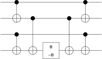
Fig. 11.: A circuit for the phase shift $\theta\mu_{s}$, i.e. a phase shift of $+\theta$ if the number of true qubits is even and $-\theta$ if it is odd.

It is easy to see that the $\mu_{s}$ for all $s\subset\{1,\ldots,n\}$ are linearly independent, and form a basis of ${\mathbb{R}}^{2^{n}}$. Moreover, while diagonal gates coupling $k$ qubits can only perform phase shifts spanned by those $\mu_{s}$ with $|s|\leq k$, the circuit in figure 11 can perform a phase shift proportional to $\mu_{s}$ for any $s$ (incidentally, in depth ${\cal O}(\log|S|)$ with no ancillae). Therefore, a series of $2^{n}$ such circuits, one for each subset of $\{1,\ldots,n\}$, can express any diagonal unitary operator. ∎

Then we have the following corollary:

Corollary 5.17.

There are circuits composed of controlled-not gates and one-qubit diagonal gates that cannot be parallelized to less than exponential depth with a polynomial number of ancillae.

Proof 5.18.

Consider setting up a many-to-one correspondence between circuits and operators. The set of diagonal unitary operators on $n$ qubits has $2^{n}$ continuous degrees of freedom, while the set of circuits of depth $d$ and $m$ ancillae has only ${\cal O}(d(m+n))$ continuous degrees of freedom (and some discrete ones for the circuit’s topology). Thus if $m$ is polynomial, $d$ must be exponential. ∎

Note that this counting argument does not help us distinguish ${\bf QP}$ from ${\bf QNC}$, since both have a polynomial number of degrees of freedom. Neither does it help us exhibit a particular family of circuits which require exponential depth, since it is completely non-constructive. The classical situation is similar; there are $2^{2^{n}}$ Boolean functions on $n$ variables, but only $2^{{\cal O}(dw\log w)}$ circuits of depth $d$ and width $w$. Thus the vast majority of Boolean functions require exponential depth if the width is polynomial, but proving a lower bound on the depth of a particular one remains elusive.

6 ${\bf QNC}\neq{\bf QP}$? The staircase circuit

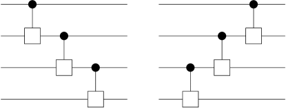
Fig. 12.: This “staircase” circuit seems hard to parallelize unless the operators are purely diagonal or off-diagonal.

A simple, perhaps minimal, example of a quantum circuit that seems hard to parallelize is the “staircase” circuit shown in figure 12. This kind of structure appears in the standard circuit for the quantum Fourier transform, which has ${\cal O}(n^{2})$ gates [2, 8]. Careful inspection shows that the QFT can in fact be parallelized to ${\cal O}(n)$ depth as shown in figure 13 [5], but it seems difficult to do any better. Clearly, any fast parallel circuit for the QFT would be relevant to prime factoring and other problems the QFT is used for.

If we define ${\bf QP}$ as the family of quantum operators that can be expressed with circuits of polynomial depth (again, leaving measurement issues aside for now), we can make the following conjecture:

Conjecture 6.19.

Staircase circuits composed of controlled-$U$ gates other than diagonal or off-diagonal gates (i.e. other than the special cases handled in propositions 3.11 and 4.13) cannot be parallelized to less than linear depth. Therefore, ${\bf QNC}<{\bf QP}$.

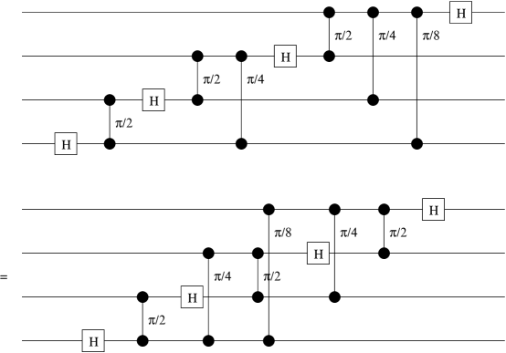
Fig. 13.: The standard circuit for the quantum Fourier transform on $n$ qubits can be carried out in $2n-1$ layers. Can we do better?

7 Conclusion

We conclude with some questions for further work.

Parsing classical context-free languages is in ${\bf NC}$. Quantum context-free languages have been defined in [6]. Is quantum parsing, i.e. producing derivation trees with the appropriate amplitudes, in ${\bf QNC}$?

Can circuits for quantum error correction such as those in [3] be parallelized to significantly smaller depth? If so, does this reduce the threshold error necessary for long-term computation, at least as far as storage errors are concerned?

Finally, can the reader show that the staircase circuit cannot be parallelized, thus showing that ${\bf QNC}<{\bf QP}$? This would be quite significant, since corresponding classical question ${\bf NC}<{\bf P}$ is still open.

Acknowledgments. M.N. would like to thank the Santa Fe Institute for their hospitality, and Spootie the Cat for her affections. C.M. would like to thank the organizers of the First International Conference on Unconventional Models of Computation in Auckland, New Zealand, as well as Seth Lloyd, Tom Knight, David DiVincenzo and Artur Ekert for helpful conversations. He would also like to thank Molly Rose for inspiration and companionship. This work was supported in part by NSF grant ASC-9503162.

References

- [1] A. Barenco, C. Bennett, R. Cleve, D.P. DiVincenzo, N. Margolus, P. Shor, T. Sleator, J.A. Smolin and H. Weifurter, “Elementary gates for quantum computation.” quant-ph/9503016, Phys. Rev. A 52 (1995) 3457-3467.
- [2] D. Coppersmith, “An approximate Fourier transform useful in quantum factoring.” IBM Research Report RC 19642.
- [3] D.P. DiVincenzo and P.W. Shor, “Fault-tolerant error correction with efficient quantum codes.” quant-ph/9605031.
- [4] M. Frank, C. Vieri, M.J. Ammer, N. Love, N.H. Margolus, and T.F. Knight. “A scalable reversible computer in silicon.” In the proceedings of the First International Conference on Unconventional Models of Computation, Springer-Verlag, 1998.
- [5] R.B. Griffiths and C.-S. Niu, “Semiclassical Fourier transform for quantum computation.” quant-ph/9511007, Phys. Rev. Lett. 76 (1996) 3228-3231.
- [6] C. Moore and J.P. Crutchfield, “Quantum automata and quantum grammars.” quant-ph/9707031, submitted to Theoretical Computer Science.
- [7] C.H. Papadimitriou, Computational Complexity. Addison-Wesley, 1994.
- [8] P.W. Shor, “Algorithms for quantum computation: discrete logarithms and factoring.” In Proc. 35th Symp. on Foundations of Computer Science (1994) 124–134.
- [9] We are grateful to John Rickard, Ahto Truu, Sebastian Egner, and David Christie for pointing this out.