Exact boundary conditions at finite distance for the time-dependent Schrödinger equation

Abstract

Exact boundary conditions at finite distance for the solutions of the time-dependent Schrodinger equation are derived. A numerical scheme based on Crank-Nicholson method is proposed to illustrate its applicability in several examples.

I Introduction

The time-dependent quantum mechanics formalism has been extensively used in the recent years in several problems of physics and chemistry. Since the work of McCullough and Wyatt [1] showing the interest of dealing directly with non-stationary states in calculating reactions probabilities, a consequent number of works has been devoted to the wave-packet dynamics. The reader could find the more recent developments in the reviews [2, 3, 4, 5] and references therein.

When solving the time-dependent Schrödinger equation in a finite volume, one is faced with the problem of implementing the proper boundary conditions at finite distance. These boundary conditions are usually those of a free wave outgoing propagation. For the stationary solutions they are given by fixing the value of the logarithmic normal derivative on the boundaries of the interaction domain. However for the case of non-stationary wave packets a satisfactory solution is not known.

The usual way to overcome this difficulty is to impose the nullity of the wave on the boundaries and push them far enough to avoid the effect of parasite reflections in the region of interest [6]. Another way, widely used in other branches of physics and mechanics as well, is by means of the so-called absorbing boundary conditions [7, 8, 9]. They indeed minimize parasit reflections but perturbe the dynamics near the boundary and do not provide a solution of the initial equation in its neighborhood.

A third way is by the so called wave function splitting algorithm which consists in removing from the total wavefunction the part localized outside the interaction region before it reaches the boundary [10]. Other possibilities based on the interaction picture formalism have also been developed [11].

Although the above quoted methods provide a practical way to solve the problem they do not give a theoretical solution of it. The aim of this paper is to formulate an exact boundary condition (EBC) at finite distance for outgoing solutions of the time-dependent Schrödinger equation. Consequently, it would allow a solution of time-dependent quantum mechanical problems in a finite spatial domain without any approximation in the boundaries. This theoretical result is completed by implementing the derived boundary conditions in some practical calculations concerning the more usual problems of the wavepacket dynamics.

The paper is organized as follows: in Section 2 we derive the general expression for the EBC which has to be imposed at the boundary of an arbitrary integration domain containing the interaction. This conditions turns to be non local on time and allows a solution limited to the interaction domain of the time-dependent Schrödinger equation. In Section 3 the boundary conditions are reformulated for a discrete-time evolution problem in the frame of the Crank-Nicholson scheme. Section 4 is devoted to the one dimensional Schrödinger equation for which the use of these conditions is particularly simple. Several illustrative examples are given in Section 5: the spreading of a free wave packet, the scattering of a wavepacket on a static potential, the behavior of an initially localized wave packet under a time-dependent perturbation. In the last example we derive explicit solutions of the Schrödinger equation in a time-dependent delta potential. The applicability of the formulated conditions in a two-dimensional problem is shown in Section 6. A discussion on the interest and limitations of the EBC is finally presented in the conclusion.

II Boundary conditions at finite distance for the time-dependent Schrödinger equation

Let us consider the dimensionless time-dependent Schrödinger equation in a d-dimensional configuration space

$$\left[i\partial_{t}+\nabla_{\vec{x}}^{2}-V(\vec{x},t)\right]\Psi(\vec{x},t)=0$$ (1)

The potential $V$, eventually time-dependent, is assumed to vanish outside a finite domain $D_{I}$ named the interaction domain.

We wish to obtain a solution of (1) by solving the equation in a finite spatial region $D_{i}$, called hereafter the integration domain. The domain $D_{i}$ has to be chosen such that it contains $D_{I}$, i.e. such that its complementary $D_{e}$ with respect to the total configuration space $D$ is free of interaction. We have thus $D=D_{i}\bigcup D_{e}$ and $D_{I}\subseteq D_{i}$ ( see figure 1).

The solution of (1) in $D_{i}$ requires to formulate and implement the proper boundary conditions on its border, a surface $\Sigma$. For this purpose let us first consider the solution $\Psi$ of (1) in $D_{e}$. The domain $D_{e}$ is, by definition, free of interaction and $\Psi$ satisfies the free Schrödinger equation

$$(i\partial_{t}+\nabla_{\vec{x}}^{2})\Psi(\vec{x},t) = 0$$ (2)

Let $K_{0}^{+}$ be the free retarded propagator, i.e. a solution of

$$(-i\partial_{t}+\nabla_{\vec{x}}^{2})K_{0}^{+}(\vec{x_{0}}-\vec{x},t_{0}-t) = i\delta(\vec{x_{0}}-\vec{x})\delta(t_{0}-t)$$ (3)

with $\vec{x}\in D_{e}$ and $(\vec{x}_{0},t_{0})$ arbitrarily chosen.

We have in mind the outgoing solution at $(\vec{x}_{0},t_{0})$ of a time-dependent problem with initial value given by $\Psi(\vec{x},t_{i})$ for $t_{i}<t_{0}$. By multiplying equation (2) by $K_{0}^{+}$, equation (3) by $\Psi$ and substracting one gets the relation

$$\Psi(\vec{x},t)\delta(\vec{x}_{0}-\vec{x})\delta(t_{0}-t) = -\partial_{t}\left[K_{0}^{+}(\vec{x}_{0}-\vec{x},t_{0}-t)\Psi(\vec{x},t)\right]$$ (4)

$$- \nabla_{\vec{x}}\cdot\left[i\Psi(\vec{x},t)\stackrel{{\scriptstyle\leftrightarrow}}{{\nabla}}_{\vec{x}}K_{0}^{+}(\vec{x}_{0}-\vec{x},t_{0}-t)\right]$$ (5)

with $f{\stackrel{{\scriptstyle\longleftrightarrow}}{{\nabla}}}g=f(\vec{\nabla}g)-(\vec{\nabla}f)g$.

This relation is to be integrated over the $d+1$ dimensional space-time volume $D_{e}\times[t_{i},+\infty]$. We will assume that the domain $D_{e}$ is connected. This assumption is justified for most of the cases except for $d=1$, which will be discussed later. The integral of the right hand side is then transformed, by using the Green theorem, into a flux term through the boundary surface $\Sigma$. We denote by $\vec{n}$ the normal to $\Sigma$ pointing towards $D_{e}$ (see figure 1).

Taking into account that $K_{0}^{+}(\vec{x_{0}}-\vec{x},t_{0}-t)=0$ for t$>t_{0}$ and that there is no contribution from the flux at the infinity for purely outgoing waves (for they have the same asymptotic behavior as the retarded free propagator) we obtain the following relations depending on the relative position of $\vec{x}_{0}$.

If $\vec{x}_{0}\in D_{e}$ one has

$$\Psi(\vec{x_{0}},t_{0})=\int_{D_{e}}K_{0}^{+}(\vec{x_{0}}-\vec{x},t_{0}-t_{i})\Psi(\vec{x},t_{i})d\vec{x}$$ (6)

$$+i\int_{t_{i}}^{t_{0}}dt\int_{\Sigma}\Psi(\vec{x},t){\stackrel{{\scriptstyle\longleftrightarrow}}{{\nabla}}}K_{0}^{+}(\vec{x_{0}}-\vec{x},t_{0}-t).\vec{n}dS$$ (7)

The solution in the free region is thus obtained as a sum of a first term, representing the free propagation of the wave which was initially in the non interacting region $D_{e}$, and a second term made only with the values of the wavefunction and its normal derivative at the boundary $\Sigma$ at the past times. Equation (6) can be consequently used to propagate outside $D_{i}$ a solution obtained in $D_{i}$ and can be viewed as a generalization of the Huyghens principle in a space-time surface.

If $\vec{x}_{0}\in\Sigma$ one has

$${1\over 2}\Psi(\vec{x_{0}},t_{0})=\int_{D_{e}}K_{0}^{+}(\vec{x_{0}}-\vec{x},t_{0}-t_{i})\Psi(\vec{x},t_{i})d\vec{x}$$ (8)

$$+i\int_{t_{i}}^{t_{0}}dt\int_{\Sigma}\Psi(\vec{x},t){\stackrel{{\scriptstyle\longleftrightarrow}}{{\nabla}}}K_{0}^{+}(\vec{x_{0}}-\vec{x},t_{0}-t).\vec{n}dS$$ (9)

This result can be obtained either as a limiting case of the preceding one (6) or by directly integrating equation (4) for $\vec{x}_{0}\in\Sigma$. Equation (8) is the boundary condition we were looking for. It provides an integral relation between the value of the wavefunction on a point of $\Sigma$ at a given time and the values of the wavefunction and their derivatives in $\Sigma$ at the preceding times. Starting from a known initial state at time $t_{i}$, equation (8) gives in its differential form the boundary condition on $\Sigma$ required for determining at time $t_{i}+\Delta t$ the solution of the time-dependent Schrodinger equation in the finite domain $D_{i}$.

Several comments are in order:

• The relation (8) is non local in both space and time. It generalizes the outgoing boundary condition for the monochromatic free plane waves, which in the one-dimensional case and at $x=a$ reads:

  $$\Psi(a,t_{0})={1\over ik}\partial_{x}\Psi(a,t_{0})$$ (10)

• The choice of $K_{0}^{+}$ ensures that only free outgoing waves will propagate across $\Sigma$, in the same way as a solution obtained in an infinite domain. This result is exact and consequently will not generate any reflection on the boundary.

• The first term of its right hand side corresponds to the free propagation of the initial state which was initially in the external region $D_{e}$. Its numerical calculation needs some care due to the oscillatory character of the propagator and several ways to overcome it are proposed below:

  • It is always possible to eliminate this contribution by choosing the initial time $t_{i}$ and $D_{i}$ in such a way that the initial state is fully in $D_{i}$.

  • In the case when the initial state is very extended, it is more suitable to include it entirely in $D_{e}$. Indeed the volume integral term gives then the value at the boundary of a free evolution of the initial state. This can be easily calculated in the momentum space and is known analytically for some cases of physical interest like gaussian wavepackets.

  • In the case when the initial state is entirely in $D_{e}$, there exists another possibility to remove the volume term by splitting the solution into its non perturbed and scattered parts, i.e.

    
    

    $\displaystyle\Psi=\Phi+\chi$

    in which $\Phi$ is the solution of (2) which coincides at $t=t_{i}$ with the initial state and $\chi$ a solution of the inhomogeneous equation

    $$\left[i\partial_{t}+\nabla_{\vec{x}}^{2}\right]\chi(\vec{x},t)=V(\vec{x},t)\Phi(\vec{x},t)$$ (11)

    The unknown function $\chi$ vanishes at $t=t_{i}$ and satisfies in the free domain $D_{e}$ the same equations than $\Psi$. It will consequently satisfy on $\Sigma$ the boundary conditions (8) without the volume term.

The preceding relations, completed by the case $\vec{x}_{0}\in D_{i}$, are summarized in the following equation

$$\epsilon\Psi(\vec{x_{0}},t_{0})=\int_{D_{e}}K_{0}^{+}(\vec{x_{0}}-\vec{x},t_{0}-t_{i})\Psi(\vec{x},t_{i})d\vec{x}$$ (12)

$$+i\int_{t_{i}}^{t_{0}}dt\int_{\Sigma}\Psi(\vec{x},t){\stackrel{{\scriptstyle\longleftrightarrow}}{{\nabla}}}K_{0}^{+}(\vec{x_{0}}-\vec{x},t_{0}-t).\vec{n}dS$$ (13)

with $\epsilon$ defined by

$\displaystyle\epsilon(\vec{x}_{0})=\left\{\begin{array}[]{lll}1&{\rm if}&\vec{x}_{0}\in D_{e}\cr 0&{\rm if}&\vec{x}_{0}\in D_{i}\cr{1\over 2}&{\rm if}&\vec{x}_{0}\in\Sigma\end{array}\right.$

The above derivation has been done under the assumption that the potential $V$ vanishes outside a finite domain $D_{I}$. This condition can be however weakened in some cases. For instance in the case of an interaction made of one short range part $V_{s}$ plus a static long range part $V_{L}$ (e.g. Coulomb, polarisation or centrifugal potentials) the same derivation holds. The interaction domain is then defined by $V_{s}$ whereas $D_{e}$ can contain $V_{L}$ all across. The only difference in equation (12) consists in replacing the free propagator $K_{0}^{+}$ by the corresponding propagator of the long range potential $V_{L}$.

In the one dimensional case the interaction domain is $D_{i}=[-a,a]$ and the free exterior domains $D_{e}$ has two connected components $[-\infty,-a]$ and $[a,\infty]$. The boundary condition (12), based on the Green theorem, has to be applied to each of them. Let us take for instance $D^{+}_{e}=[a,\infty]$. At $x_{0}=a$, the normal derivative of the free propagator on the boundary vanishes, as it can be explicitely checked on its expression ($\hbar=2m=1$):

$$K_{0}^{+}(a-x,t_{0}-t)=\Theta(t_{0}-t){1\over\sqrt{4i\pi(t_{0}-t)}}e^{{i\over 4}{(a-x)^{2}\over t_{0}-t}}$$ (14)

The EBC (8) becomes simply

$${1\over 2}\Psi(a,t_{0})=\int_{a}^{\infty}K_{0}^{+}(a-x,t_{0}-t_{i})\Psi(x,t_{i})dx-\int_{t_{i}}^{t_{0}}dt\sqrt{\frac{i}{4\pi(t_{0}-t)}}\partial_{x}\Psi(x,t)|_{a}$$ (15)

It is worth noticing that in case $t_{i}=-\infty$ this result may be obtained in a quite straightforward way. Indeed let us consider the Fourier energy components of the wavefunction

$$\Psi(x,t_{0})=\int_{-\infty}^{+\infty}d\omega\Psi(x,\omega)e^{-i\omega t_{0}}$$ (16)

and let us impose to each of them the plane wave outgoing boundary condition (10) on the form

$\displaystyle i\sqrt{\omega}\Psi(a,t_{0})=\partial_{x}\Psi(a,t_{0})$

Inserting this relation in (16) one gets

$$\Psi(a,t_{0})=\int_{-\infty}^{+\infty}dt\int_{-\infty}^{+\infty}d\omega\frac{e^{-i\omega(t_{0}-t)}}{2i\pi\sqrt{\omega}}\partial_{x}\Psi(a,t)$$ (17)

We recognize the Fourier transform of the free Green function for zero argument

$$K_{0}^{+}(x,\omega)=-i\int_{-\infty}^{+\infty}dt\;e^{-i\omega t}K_{0}^{+}(x,t)={1\over 2i\sqrt{\omega}}e^{i\sqrt{\omega}|x|}$$ (18)

and we obtain the following relation:

$$\Psi(a,t_{o})=-\int_{-\infty}^{t_{0}}dt\sqrt{{i}\over{\pi(t_{0}-t)}}\partial_{x}\Psi(a,t)$$ (19)

in agreement with the second term in the right hand side of (15). The first term does not contribute in the limit $t_{i}\rightarrow-\infty$ due to the fact that the free propagator tends to zero.

The boundary condition (12) generalizes the KKR [12] method which provides a relation between the solution and its normal derivative at the boundary of a free domain. This method has been derived and successfully applied in the case of static quantum billards. The formulation we have developed in this section appears as a natural extension of this method for space-time billards.

The condition (12) is not directly useful in a numerical solution of the problem. Indeed the singularity of the propagator at $t=t_{0}$ would generate instabilities when the dependent Schrödinger equation is discretized. To overcome this difficulty one has to reformulate the boundary conditions in the particular approximate scheme chosen. The aim of the following section is to obtain such a formulation in the frame of the Crank-Nicholson scheme.

III Boundary conditions in the Crank-Nicholson scheme

The Cranck-Nicholson [13] method for solving a discrete-time evolution problem consists in approximating the infinitesimal evolution operator

$\displaystyle{\left|{\Psi(t+\Delta t)}\right\rangle}=e^{-i{H\over\hbar}\Delta t}{\left|\Psi(t)\right\rangle}$

by the expression:

$$(1+{iH\over 2\hbar}\Delta t){\left|\Psi_{m}\right\rangle}=(1-{iH\over 2\hbar}\\ \Delta t){\left|\Psi_{m-1}\right\rangle}$$ (20)

where ${\left|\Psi_{m}\right\rangle}$ and ${\left|\Psi_{m-1}\right\rangle}$ are the wavefunctions at two consecutive times separated by $\Delta t$ and the hamiltonian H is evaluated at the mean time $t+{\Delta t\over 2}$.

By introducing the imaginary parameter $\mu^{2}=\frac{4im}{\hbar\Delta t}$, equation (20) can be rewritten in the form

$$(\mu^{2}-H)\Psi_{m}=(\mu^{2}+H)\Psi_{m-1}$$ (21)

according to what the solution at time-step m is obtained by solving an inhomogeneous stationary Schrödinger equation with complex energy $\mu^{2}$. The source term is provided by the solution at the preceding time.

By means of (21) the equivalent of equation (2) for the outgoing wavefunction in the free domain $D_{e}$ becomes

$$\mu^{2}(\Psi_{m}-\Psi_{m-1})=-\nabla_{\vec{x}}^{2}(\Psi_{m}+\Psi_{m-1})$$ (22)

and the discrete free retarded propagator $K_{p}(\vec{x_{0}}-\vec{x})$ is defined as the solution of

$$\mu^{2}(K_{p+1}-K_{p})=-\nabla_{\vec{x}}^{2}(K_{p+1}+K_{p})$$ (23)

normalised to $K_{0}(\vec{x_{0}}-\vec{x})=\delta(\vec{x_{0}}-\vec{x})$

For $\vec{x}_{0}\notin\Sigma$ one obtains the analogous to the continuum case by simply replacing the time integral by a sum over the discrete index p

$$\epsilon\Psi_{n}(\vec{x_{0}}) = \int_{D_{e}}K_{n}(\vec{x_{0}}-\vec{x})\Psi_{0}(\vec{x})dV$$ (24)

$$+ \frac{1}{2\mu^{2}}\sum\limits_{p=0}^{n-1}\int_{\Sigma}\left[\left(K_{p}(\vec{x}-\vec{x}_{0})+K_{p+1}(\vec{x}-\vec{x}_{0})\right){\stackrel{{\scriptstyle\longleftrightarrow}}{{\nabla}}}\left(\Psi_{n-p}(\vec{x})+\Psi_{n-p-1}(\vec{x})\right)\right]\vec{n}dS$$ (25)

In calculating the limit $\vec{x_{0}}\rightarrow\Sigma$ and like in the continuum case there is a singularity in the normal derivative of the free propagator. Its contribution to the surface term in the r.h.s of (24) is

$\displaystyle\frac{1}{2}\sum\limits_{p=0}^{n-1}(-1)^{p}(\Psi_{n-p}(\vec{x_{0}})+\Psi_{n-p-1}(\vec{x_{0}}))=\frac{1}{2}\left(\Psi_{n}(\vec{x_{0}})+(-1)^{n}\Psi_{0}(\vec{x_{0}})\right)$

for $\vec{x_{0}}\in D_{e}$ and the opposite for $\vec{x_{0}}\in D_{i}$. The volume contribution can be in its turn re-written by means of the regularized propagator $\tilde{K}_{p}$ defined as

$$K_{p}(\vec{X})=(-1)^{p}\delta(\vec{X})+\tilde{K}_{p}(\vec{X})$$ (26)

and one finally arrives to

$${1\over 2}\Psi_{n}(\vec{x_{0}}) = \int_{D_{e}}\tilde{K}_{n}(\vec{x_{0}}-\vec{x})\psi_{0}(\vec{x})dV$$ (27)

$$+ \frac{1}{2\mu^{2}}\sum\limits_{p=0}^{n-1}\int_{\Sigma}\left[\left(\tilde{K}_{p}(\vec{x}-\vec{x_{0}})+\tilde{K}_{p+1}(\vec{x}-\vec{x}_{0})\right){\stackrel{{\scriptstyle\longleftrightarrow}}{{\nabla}}}\left(\Psi_{n-p}(\vec{x})+\Psi_{n-p-1}(\vec{x})\right)\right]\vec{n}dS$$ (28)

This expression is the equivalent of (8) for the discrete time evolution.

To make use of the discrete EBC condition (27) it remains to derive an expression for the discrete-time free propagator $K_{p}$. In the momentum space equation (23) reads as

$\displaystyle K_{p+1}(\vec{k})=\left(\frac{\mu^{2}+k^{2}}{\mu^{2}-k^{2}}\right)K_{p}(\vec{k})$

which leads to:

$$K_{p}(\vec{k})=\left(\frac{\mu^{2}+k^{2}}{\mu^{2}-k^{2}}\right)^{p}$$ (29)

One can see in equation (29) that in the limit $k\rightarrow\infty$ the Fourier transform of the propagator contains the singular delta function manifested in (26). Nevertheless this term cancels in the sum of two successive propagators. This sum is given by the non singular integral:

$$K_{p}(\vec{X})+K_{p+1}(\vec{X})=\int\frac{2\mu^{2}}{\mu^{2}-k^{2}}\left(\frac{\mu^{2}+k^{2}}{\mu^{2}-k^{2}}\right)^{p}e^{i\vec{k}\vec{X}}\frac{d\vec{k}}{(2\pi)^{d}}$$ (30)

This integral can in principle be calculated by the contour Cauchy method. However, its value can also be obtained by means of the discrete Fourier tranform. We note indeed that a N discrete-time Fourier transfom with respect to the index p of equation (30) gives the sum of a geometric series. With the inverse Fourier transform we obtain:

$$K_{p}(x)+K_{p+1}(x)=\frac{1}{N}\sum\limits_{l=0}^{N-1}\frac{e^{-ip\phi_{l}}}{1+e^{i\phi_{l}}}G_{0}^{+}(k_{l}^{2},x)$$ (31)

where $\phi_{l}=\frac{2l\pi}{N}+i\eta$ and $\eta$ is the required convergence factor of the geometric series which has to be chosen such that $e^{-N\eta}<<1$. $G_{0}^{+}$ is the standard free Green function with energy $k_{l}^{2}=\mu^{2}\frac{1-e^{i\phi_{l}}}{1+e^{i\phi_{l}}}$.

Although the formalism has been developed in view of solving the Schrodinger equation in a finite domain $D_{i}$, equation (24) with $\epsilon=1$ provides the wavefunction in all the configuration space. However one can obtain a closed form for some observables in terms of the internal solution only. Let us consider for example the overlapping between two outgoing solutions $\Phi$ et $\Psi$ of (22) in the exterior domain. Standard algebra gives for the exterior part of the integral the expression

$${\left\langle\left.{\Phi}\right|{\Psi}\right\rangle}_{e}^{n}-{\left\langle\left.{\Phi}\right|{\Psi}\right\rangle}_{e}^{n-1}=\frac{1}{2\mu^{2}}\int(\Phi_{n}+\Phi_{n-1})^{*}{\stackrel{{\scriptstyle\longleftrightarrow}}{{\nabla}}}(\Psi_{n}+\Psi_{n-1})\vec{n}dS$$ (32)

which can be calculated from the solution in $D_{i}$. By adding the corresponding equations for consecutive time steps one obtains the desirate scalar product. This expression is used e.g. in calculating the auto-correlation function (see section IV E). The case $\Phi_{n}=\Psi_{n}$ provides the rate of variation of the probability in the exterior domain by time step. The contribution from $D_{i}$ can be calculated by numerical integration and we thus have the possibility to verify the conservation of the total norm .

In summary the solution of the time dependent Schrödinger equation in the interaction domain $D_{i}$ can be obtained by solving, at each time step, a stationary complex and inhomogeneous Schrödinger equation (20) in $D_{i}$ with the boundary conditions given by (27). The local character of this equation is preserved by these conditions. We are thus let with the solution of a banded linear system, whatever the discretisation algorithm used for the spatial variables. For static hamiltonians this linear system is in addition the same at any time-step.

IV Examples in the one dimensional case

In the one dimensional problems, simplifications arise. Like in the continuum case, the normal derivatives of the propagator at the boundaries vanish. The sum of two successive propagators for $x_{0}=a$ can be explicitly calculated and gives:

$$K_{p}(0)+K_{p+1}(0)=\int\frac{2\mu^{2}}{\mu^{2}-k^{2}}\left(\frac{\mu^{2}+k^{2}}{\mu^{2}-k^{2}}\right)^{p}\frac{dk}{2\pi}$$ (33)

This integral can be performed by standard methods: it vanishes for odd values of p and for $p=2q$ it gives

$$K_{2q}(0)+K_{2q+1}(0)=-i\mu C_{q}$$ (34)

with

$\displaystyle C_{q}=\frac{(2q)!}{(2^{q}q!)^{2}}$

The boundary conditions (27) give at $x_{0}=a$:

$$\Psi_{n}(a)=2\int_{a}^{\infty}\tilde{K}_{n}(x-a)\Psi_{0}(x)dx-{i\over\mu}\sum\limits_{q=0}^{[{n-1\over 2}]}C_{q}\partial_{x}\left[\Psi_{n-2q}(a)+\Psi_{n-2q-1}(a)\right]$$ (35)

At $x_{0}=-a$ one obtains in a similar way

$$\Psi_{n}(-a)=2\int^{-a}_{-\infty}\tilde{K}_{n}(x+a)\Psi_{0}(x)dx+{i\over\mu}\sum\limits_{q=0}^{[{n-1\over 2}]}C_{q}\partial_{x}\left[\psi_{n-2q}(-a)+\Psi_{n-2q-1}(-a)\right]$$ (36)

For illustration we have detailed some simple examples concerning the time evolution of wavepackets. The initial state has been taken for simplicity of gaussian form

$$\Psi_{0}(x)=\frac{1}{\pi^{1/4}\sigma_{0}^{1/2}}e^{i{mv\over\hbar}(x-x_{0})}\;e^{-\frac{(x-x_{0})^{2}}{2{\sigma_{0}}^{2}}}$$ (37)

The examples have been solved by scaling the integration domain $D_{i}$ to the interval $[-1,+1]$. The discrete-time Schrödinger equation (20) is there solved at each of the N time-steps by finite differences method with $N_{x}$ equally spaced grid points $x_{i}$. The values of the wave function at $x_{i}$ are the unknowns. The required $N_{x}$ equations are obtained by validating (20) at each grid point. However to evaluate the second derivative at the end of the grid the values of the wave function at the nearest points exterior of this domain is needed. These are written in terms of the internal points by using EBC conditions (35,36) with a symmetric formula to evaluate the derivative term. Substituting this exterior values in (20) we end with a tridiagonal linear system of dimension $N_{x}$.

A Free propagation of a gaussian wave packet

The first example concerns the free propagation of a gaussian wave-packet. Its main interest lies in the fact that an analytical solution is known which allows to check the validity of our boundary conditions. In this case the integration domain is not fixed by the interaction but chosen such that it fully contains the initial wavepacket.

The wave packet (37) is initially centered ($x_{0}=0$) and, in absence of interaction, the probability density at time $t$ is known to be given by :

$\displaystyle\rho(x,t)=\mid\Psi(x,t)\mid^{2}=\frac{1}{\pi^{1/2}\sigma(t)}e^{-\frac{(x-vt)^{2}}{\sigma^{2}(t)}}$

with $\sigma(t)=\sigma_{0}\sqrt{1+\tilde{t}^{2}}$ and $\tilde{t}=\frac{\hbar}{m\sigma_{0}^{2}}t$ a dimensionless time variable. If the total evolution time in this units is $\tilde{T}$, one has $\mu^{2}=\frac{4im}{\hbar\Delta t}=\frac{4iN}{{\sigma_{0}}^{2}\tilde{T}}$. We have taken for the initial width the value $\sigma_{0}=0.2$.

In figure (2) are displayed the density probabilities each 4 time steps. The time $\tilde{T}$ is equal to $4$, the number of time steps is $N=40$ and $N_{x}=201$. The wave packet velocity $v$ is chosen such that during the time $\tilde{T}$ a classical particle would travel half the interval $[-1,+1]$. The initial state is shown by dashed line. One can see by simple inspection the absence of any parasite reflection nor anomalous behavior. The curve corresponding to the time $\tilde{t}=\tilde{T}$ is compared to the analytical result. The difference is not visible by eyes except at the vicinity of $x=1$ in which it reaches its maximum value, less than 1%. This difference has been arbitrarily reduced by increasing the number of time and space grid points showing the validity of this approach. The parameters chosen in this simple example may serve to illustrate the efficiency and accuracy of this method.

In the example considered above and due to the value of $v$, the probability flux leaves the interaction domain mostly at $x=1$. However, due to the spreading of the wavepacket, the wave function at $x=-1$ is also being populated although its value remains very small and is not visible in the figure. By taking v=0 one has a symmetric situation for which the same quality of results has been obtained.

A last check has been done concerning the total probability conservation. The contribution coming from the interior domain has been obtained by integrating (trapezoidal rule) the calculated wavefunction. The contribution from the external part has been evaluated by equation (32) which becomes in that case

$$\int_{1}^{+\infty}\left(\mid\Psi_{n}(x)\mid^{2}-\mid\Psi_{n-1}(x)\mid^{2}\right)dx=\frac{1}{2\mu^{2}}(\Psi_{n}+\Psi_{n-1})^{*}\partial_{x}(\Psi_{n}+\Psi_{n-1})\mid_{x=1}$$ (38)

In this example the probability is found to be conserved better than $10^{-5}$.

B Scattering by a static potential

In the second example, the initial wave packet (37) scatters on an attractive potential:

$\displaystyle V(x)=V_{0}e^{-{x^{2}\over b^{2}}}$

with $b=0.05$ and $V_{0}=-150$. The wavepacket parameters are $x_{0}=-0.3$, $\sigma_{0}=0.15$, $v=0.37$.

The probability densities at different times are displayed in figure (3). Its initial value is plotted in dashed line and the attractive well in bold. The reflected and transmitted wave packets are clearly separated. The integrated probabilites in $D_{e}$ and $D_{i}$ have been calculated respectively by (38) and trapezoidal rule from the solution in $D_{i}$. They are shown as a function of time in figure (4). The contribution from the $x<-1$ and $x<1$ regions are respectively plotted in curves (a) and (b). They correspond to the reflected and transmitted wavepackets. The difference between both curves corresponds to the integrated probability in the integration domain. It tends to zero very slowly.

C Localized state under a time-dependent perturbation

The third example concerns the evolution of a wave packet initially localized on an attractive gaussian potential whose amplitude varies periodically:

$$V(x,t)=V_{0}\left(1+\sin 2\pi\omega\tilde{t}\right)\;e^{-{x^{2}\over b^{2}}}$$ (39)

with $b=0.05$, $\omega=0.05$ and $V_{0}=-200$.

The time of evolution is T=80, with 800 points in space and 800 time-steps. The initial state is a superposition of the bound states plus a small component ($\approx 3\%$) of continuum states both in the corresponding static potential at $t=0$. Curves (a) and (b) on figure (5) represent respectively the probability density in the intervals $x<-1$ and $x<1$. The difference between these curves, i.e. the probability density in the integration domain, tends to zero showing that the bound state is pulled out of the potential by the time dependent perturbation. The evolution in the corresponding static potential, shown in dashed lines, tends to a constant: the projection of the initial wavepacket into bound states.

D Tunneling

The following example illustrates the tunnel effect through a double well. A gaussian wavepacket with $\sigma_{0}=0.12$, initially centered and at rest $v=0$ evolves in a double repulsive well of the form

$$V=V_{0}\left[e^{-{(x-a_{0})^{2}\over b^{2}}}+e^{-{(x+a_{0})^{2}\over b^{2}}}\right]$$ (40)

with $b=0.05$ $a_{0}=0.5$ and $V_{0}=150$. We have displayed in figure (6) the probability density at different times. The initial state is drawn in dashed line and the potential (arbitrary units) in bold. The wavefunction spreads and oscillates inside the potential except for a small part that tunnels through. The time evolution of the integrated probability densities corresponding to figure (6) is shown in figure (7). Curve (a) corresponds to the domain $x<-1$ and curve (b) to $x<1$. The distance between both curves represents the integrated probability in the integration domain $D_{i}$. The small oscillations correspond to the back and forth reflections of the wavepacket inside the well.

E Time-dependent Delta potential

An interesting example is provided by the limiting case of a time-dependent delta potential

$\displaystyle V(x)=-\lambda(t)\delta(x)$

In this case the interaction domain is reduced to a point and it is possible to obtain closed analytical solutions for the discrete-time evolution problems.

We will consider the evolution of a state $\Psi$ which initially coincides with the bound state $\Phi_{0}$ of the potential with strength $\lambda_{0}$. Its energy, in current units ($\hbar=2m=1$), is $E_{0}=-\omega_{0}=-{\lambda_{0}^{2}\over 4}$ and the normalized wavefunction

$\displaystyle\Phi_{0}(x)=\sqrt{\lambda_{0}\over 2}\;e^{-{\lambda_{0}\over 2}|x|}$

By integrating the discrete-time Schrödinger equation (21) on both sides of the singularity one gets the discontinuity of the wave function derivative at $x=0$

$$\lambda_{n}\left\{\Psi_{n}(0)+\Psi_{n-1}(0)\right\})+\left[\partial_{x}(\Psi_{n}+\Psi_{n-1})\right]_{0^{-}}^{0^{+}}=0$$ (41)

where $\lambda_{n}$ is the mean intensity of the potential between the $n$ and $n-1$ time-steps.

The solution of (21) $\Psi_{n}$ will be written by splitting its non perturbed $\Phi_{n}$ and perturbed $\chi_{n}$ parts

$$\Psi_{n}=\Phi_{n}+\chi_{n}$$ (42)

By definition, $\Phi_{n}$ is a stationary solution of equation (21) with $\lambda=\lambda_{0}$. In the continuum case the time evolution of $\Phi_{n}$ would be simply given by

$\displaystyle\Phi_{n}=e^{-ni\omega_{0}\Delta t}\Phi_{0}$

In the discrete-time evolution it is easy to show that

$\displaystyle\Phi_{n}=e^{-ni\theta}\Phi_{0}$

with

$\displaystyle e^{-i\theta}={\mu^{2}-\omega_{0}\over\mu^{2}+\omega_{0}}$

The perturbated part $\chi_{n}$ is a solution of (22) on both sides of $x=0$ and satisfies the boundary conditions (35). The sum of these two conditions gives

$$2\chi_{n}(0)=-\frac{i}{\mu}\sum\limits_{q=0}^{{n-1\over 2}}C_{q}\left[\partial_{x}(\chi_{n-2q}+\chi_{n-2q-1})\right]_{0^{-}}^{0^{+}}$$ (43)

Combining this last result with equations (41) and (42) one obtains at x=0

$$2\chi_{n}=\frac{i}{\mu}\sum\limits_{q=0}^{{n-1\over 2}}C_{q}\left[\lambda_{n}(\chi_{n-2q}+\chi_{n-2q-1})+(\lambda_{n}-\lambda_{0})(\Phi_{n-2q}+\Phi_{n-2q-1})\right]$$ (44)

This is an inhomogeneous linear system for the perturbed wave function $\chi_{n}$ with the inhomogeneous term given by $\Phi_{n}$. By isolating the q=0 contribution equation (44) results into an explicit recurrence relation

$$(-2i\mu-\lambda_{n})\chi_{n}=\lambda_{n}\chi_{n-1}+\sum\limits_{q=1}^{{n-1\over 2}}C_{q}\lambda_{n}(\chi_{n-2q}+\chi_{n-2q-1})+\sum\limits_{q=0}^{{n-1\over 2}}C_{q}(\lambda_{n}-\lambda_{0})(\Phi_{n-2q}+\Phi_{n-2q-1})$$ (45)

The perturbed wave function $\chi_{n}$ at the origin can be thus easily obtained. The values at $x\neq 0$ can be calculated from equations (24) and (31) This example illustrates how we can extract all the physical quantities from the knowledge of the wave function and its derivative on the boundary, even in a limiting case when it is reduced to a point.

In figure (8) are displayed the results corresponding to a periodically driven delta potential with

$\displaystyle\lambda(t)=\lambda_{0}+{A\over 2}\left\{1-\cos\left({0.7\omega_{0}t}\right)\right\}$

and where $\omega_{0}$ is the Bohr frequency of the bound state for $\lambda=\lambda_{0}$. Curve (a) shows the square modulus of the auto-correlation function $<\Phi(t)|\Psi(t)>$ and curve (b) the square modulus of the wave function at the origin normalized to one at the initial time. For the long times the wave function near the origin becomes proportional to the bound state and these two quantites are close to each other. There are 1000 time steps for 40 perturbative pulses. We note that after a transient period, the wave function is near of an eigenvector of the Floquet operator [14] with complex energy.

The periodically driven delta potential is used as a model of weakly bound atom (1D delta atom) when studying the tunnel effect in a static exterior field [15]. In this case the exact propagator is known explicitly. In our case there is also an explicit solution.

V A two dimensional example

We present in this section a straightforward application of the formulated boundary conditions for a two dimensional problem. We will illustrate it by considering the free evolution of a two dimensional gaussian wave packet crossing obliquely the $x=1$ axis. The wave packet has initial widths $\sigma_{0x}=\sigma_{0y}=0.2$ and is initially centered at the point $(0,1)$ of the XY plane with velocity $v_{y}/v_{x}=3/2$. We push to the infinity the domain for the y variable and consider as integration domain the band $D_{i}=[-1,+1]\times{\bf R}$

Let us apply the boundary conditions (27) to a point $x_{0}$ in the line $\gamma_{a}=\{(a,y)\in R^{2}:y\in(-\infty,+\infty)\}$. The integral term has only contributions coming from $\gamma_{a}$ itself and is thus reduced to a one- dimensional integral although with a two- dimensional propagator of non-vanishing argument $K_{p}(\vec{X})$.

$${1\over 2}\Psi_{n}(a,y_{0})={1\over 2\mu^{2}}\sum_{p=0}^{n-1}\int_{-\infty}^{+\infty}dy\;\left[\left(K_{p}(\vec{x}-\vec{x}_{0})+K_{p+1}(\vec{x}-\vec{x}_{0})\right)\nabla\left(\Psi_{n-p}(\vec{x})+\Psi_{n-p-1}(\vec{x})\right)\right]$$ (46)

with $\vec{x}=(a,y)$ and $\vec{x}_{0}=(a,y_{0})$.

An efficient way to solve (46) is by Fourier transforming the wavefunction with respect to the $y$ variable

$\displaystyle\Psi_{n}(a,y)=\int_{-\infty}^{+\infty}dk_{y}\;e^{ik_{y}y}\;\tilde{\Psi}_{n}(a,k_{y})$

and impose the desired boundary condition to each of its Fourier components $\tilde{\Psi}_{n}(a,k_{y})$. The problem is then formally equivalent to a one- dimensional one with a propagator given by expression (33) where the $k^{2}$ variable is replaced by $k^{2}+k_{y}^{2}$. The resulting integral is no longer analytic as in the one dimensional case but can be easily evaluated by means of a discrete Fourier tranform according to equation (31).

The numerical results are displayed in figure 9. They correspond to the solution of the discrete time Schrödinger equation in the region $x\in[-1,+1]$ and $y\in[0,5]$ with $N=100$ time steps. The number of points in x direction is $N_{x}=101$ and $N_{y}=45$ points were required for an accurate Fourier transform of $\Psi_{n}(a,y)$ amplitudes. The countour plots of the probability density are shown for six equidistant times.

The figure shows the spreading of the wave packet in both directions and the crossing of the $x=1$ boundary without any parasit reflections. The comparison of calculated values with the exact analytic expressions showed a relative accuracy at the maximum of the wave packet better than $1\%$.

VI Conclusion

Exact boundary conditions at finite distance for the time-dependent Schrödinger equation have been derived. These conditions allow a resolution of time-dependent quantum mechanical problems in a finite spatial domain containing the interaction without introducing any parasite reflections, nor changing the dynamics near the boundary. They are specially useful to observe long time evolution of waves packets in a finite space domain.

The value of the wavefunction outside the integration domain can be easily obtained from the values of the wave function and its normal derivative at the boundaries for all the anterior times.

These conditions have been explicitely reformulated in a time-discrete dynamics and implemented in a numerical algorithm providing a numerical solution of the more usual one-dimensional problems. They result in solving at each discrete time step a stationary Schrödinger equation with complex energy in a finite spatial domain. The local character of this equation is preserved by the boundary conditions and we are thus let with a band matrix problem whatever the discretisation algorithm used.

The economy resulting when solving the problem in a reduced spatial domain allows to considerably increase the number of grid points and to use for a same accuracy less powerful but simpler algorithms. The numerical results obtained with the Cranck Nicholson scheme are found to be very satisfactory. Other time and space discretisation algorithms can however be used as well at the cost of the simplicity.

The derived boundary conditions can be applied to more general situations than those considered in the examples. The case of higher dimensionality and/or of coupled equations, for instance, can be treated without modifying the formalism. A numerical application of the free evolution of a two-dimensional gaussian wave packet is given. Long range static potentials may be taken into account as far as an analytic solution is known for the corresponding propagators. The generalization to the time-dependent treatment of the three body problem is straightforward and could be of some interest in some molecular physics problems [17] or a doorway to solve the still open question of Coulomb problem above threshold.

The interest in formulating exact boundary conditions at finite distance for time-dependent problems recently appeared in the field of statistical mechanics and conclusions similar to those presented in this work have been reached in [18]. But this formulation is also relevant in other branches of physics than those governed by the Schrödinger equation. In particular for the diffusion equation, for which the same results hold with imaginary time. The case of hyperbolic equation of interest in many fields of physics can be treated in the same footing [16].

VII Acknowledgments

We acknowlegde Dr. K. Protassov for his support on some mathematical aspects of this work and Prof. C. Leforestier for helpful discussions.

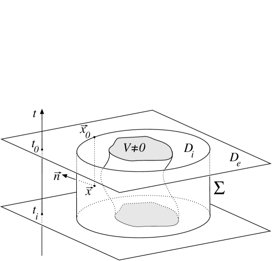
FIG. 1.: Space-time representation of different equal-time sections of the configuration space D. The shadowed region represents the interaction domain $D_{I}$. The time-dependent Schrodinger equation is solved in the finite domain $D_{i}$

FIG. 2.: Free evolution of a gaussian wave packet. It has been obtained by solving the time-dependent Schrödinger equation in a limited region of the configuration space with the boundary conditions given by (12). Dashed curve represents the probability density of the initial wavepacket for $\sigma_{0}=0.2$. The time evolution is plotted at ten different times showing the spreading of the wavepacket and its global displacement without any parasite reflections at the boundaries $x=\pm 1$

FIG. 3.: Scattering of a gaussian wavepacket on an attractive gaussian potential drawn in bold line. The initial state, in dashed line, is centered at $x_{0}=-0.3$ and has $\sigma_{0}=0.15$ and $v=0.37$. It splits into a transmitted and a reflected part which goes accross the boundaries of the integration domain without any reflection.

FIG. 4.: Time evolution of the integrated probability densities for the scattered wavepacket of figure (3). Curves (a) and (b) represent the probability density in the intervals $x<-1$ and $x<+1$, calculated by equation (38). They tend towards the corresponding transmission and reflection coefficients. This convergence is relatively slow due to the slow spreading of the initial state in the integration domain $D_{i}=[-1,+1]$.

FIG. 5.: Evolution of a localized state in the time-dependent potential (39). The initial state, a gaussian wavepacket with $\sigma_{0}=0.10,x_{0}=0,v=0$, is a superposition of bound states plus a small contribution from the continuum, both in the corresponding static potential at $t=0$. Curves (a) and (b) represent respectively the probability density in the intervals $x<-1$ and $x<1$. The difference between these curves, i.e. the probability density in the integration domain, tends to zero showing that the bound state is pulled out of the potential by the time dependent perturbation. The evolution in the correponding static potential is shown in dashed lines.

FIG. 6.: Tunneling through a double repulsive well (bold curve). The wavepacket is initially centered (dashed line) with $\sigma_{0}=0.12$ and $v=0$. It spreads and oscillates inside the potential except for a small part that tunnels through

FIG. 7.: Time evolution of the integrated probability densities corresponding to Fig. (6) are shown. Curve (a) is the integrated probability in the region $x<-1$ and curve (b) in $x<1$. The distance between both curves corresponds to the integrated probability in the integration domain $D_{i}$. The small oscillations are due to the back and forth reflections of the wavepacket inside the well.

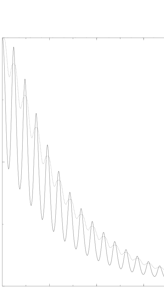
FIG. 8.: Time-evolution of a bound state in a pulsed delta potential $V(x)=-\lambda(t)\delta(x)$. Solid curve represents the probability density at the origin. Dashed curve represents the squared modulus of the autocorrelation function $|{\left\langle\left.{\Psi_{0}}\right|{\Psi_{n}}\right\rangle}|^{2}$. Abscisse units are the number of time-steps. The total time evolution corresponds to 32 Bohr periods. The frequency of the potential pulse is 7/10 the Bohr frequency.

FIG. 9.: Free evolution of a two-dimensional gaussian wave packet. It has been obtained by solving the Schrödinger equation in the displayed rectangular region, i.e. horizontal axis $x\in[-1,+1]$ and vertical axis $y\in[0,5]$, by imposing exact boundary conditions at finite distance. The countour plots of the probability density are shown for six equidistant times. The wave packet (t=1) was initially centered at $x=0$ $y=1$ with an initial momentum $v_{y}/v_{x}=3/2$. The figure shows the spreading of the wave packet in both directions and the crossing of the $x=1$ boundary without any parasite reflections.

REFERENCES

- [1] E.A. McCullough, R.E. Wyatt, J. Chem. Phys. 54, 3578 (1971)
- [2] Time-Dependent Quantum Molecular Dynamics,NATO ASI Series 299, Ed. by J. Broeckhove et al., Plenum Press 1992
- [3] M. Kleber, Phys. Rep. 236, 331 (1994)
- [4] B.M. Garraway and K.A. Suominen, Rep. Prog. Phys 58, 365 (1995)
- [5] N. Balakrishnan, C. Kalyanaraman, N. Sathyamurthy, Phys. Rep. 280, 79 (1997)
- [6] A. Goldberger, H.M. Schey, J.L. Scwwartz, Am. J. of Phys. 35 177 (1967)
- [7] C. Leforestier and R.E. Wyatt , J. Chem. Phys. 78, 2334 (1983)
- [8] R. Kosloff, D. Kosloff, J. of Comput. Phys. 63, 363 (1986)
- [9] A. Vibok, G.G. Balin-Kurti, J. Chem. Phys. 96 7615 (1992)
- [10] R. Heather and H. Metiu, J. Chem. Phys. 86, 5009 (1987); 88, 5496 (1988); R. Heather, Comput. Phys. Com. 63, 446 (1991)
- [11] J.Z.H. Zhang, Chem. Phys. Lett. 160, 417 (1989)
-
[12]
R. Balian and C. Bloch, Ann. Phys. 60, 401 (1970)
M. Berry, Ann. Phys. 131, 163 (1981) - [13] Numerical Recipes W.H. Press, S.A. Teukolsky, W.T. Vetterling, B.P. Flannery Cambridge Univ. Press New York 1986
- [14] S. H. Shirley, Phys. Rev. 138, 3979 (1965)
- [15] S. Geltman J. Phys. B 11, 3323 (1978)
- [16] O. Meplan and C.Gignoux Phys. Rev. Lett. 76 408 (1996)
- [17] C. Leforestier, F. LeQuéré, K. Yamashita, K. Morokuma, J. Chem. Phys. 101, 3806 (1994)
- [18] J. R. Hellums and W. R. Frensley, Phys. Rev. B 49, 2904 (1994)