FSUJ TPI QO-6/98

March, 1998

Quantum state engineering using conditional measurement on a beam splitter
M. Dakna, L. Knöll, D.–G. Welsch
Friedrich-Schiller-Universität Jena, Theoretisch-Physikalisches Institut

Max-Wien-Platz 1, D-07743 Jena, Germany

Abstract

State preparation via conditional output measurement on a beam splitter is studied, assuming the signal mode is mixed with a mode prepared in a Fock state and photon numbers are measured in one of the output channels. It is shown that the mode in the other output channel is prepared in either a photon-subtracted or a photon-added Jacobi polynomial state, depending upon the difference between the number of photons in the input Fock state and the number of photons in the output Fock state onto which it is projected. The properties of the conditional output states are studied for coherent and squeezed input states, and the probabilities of generating the states are calculated. Relations to other states, such as near-photon-number states and squeezed-state-excitations, are given and proposals are made for generating them by combining the scheme with others. Finally, effects of realistic photocounting and Fock-state preparation are discussed.

1 Introduction

Over the last years numerous workers have studied various nonclassical states of radiation and proposed schemes for producing them. Particular interest has been devoted, e.g., to Fock states (for a review, see [1]) and states derived from Fock states by coherently displacing and/or squeezing them [2, 3, 4, 5, 6], superpositions of mesoscopically distinguishable states, such as Schrödinger-cat-like states (for a review, see [7]), near-photon-number states (also called crescent states) [8, 9, 10, 11, 12, 13], binomial states [14, 15, 16], inverse binomial states [17, 18], squeezed-state excitations [19, 20] and the SU(2) and SU(1,1) minimum-uncertainty states [10, 21, 22]. Another interesting class of nonclassical states that have been a subject of increasing interest are photon-added and photon-subtracted states that are obtained by repeated application of photon creation or destruction operators, respectively, on a given state [23, 24, 25, 26, 27, 28, 29, 30]. Similarly, states obtained by the repeated application of the inverse boson operators have also been considered [31].

Despite the large body of work, only few of the above mentioned nonclassical states have been generated experimentally so far. Designing of realistic schemes for generating specific quantum states and realization of the schemes in the laboratory have been one of the most exciting challenges to the researchers. A promising method of quantum state engineering has been conditional measurement, e.g., generation of a desired state by state reduction in one of two entangled quantum objects owing to an appropriate measurement on the other object. Typical examples that have been considered for nonclassical state generation via conditional measurements are the interfering fields in the output channels of a beam splitter [23, 24, 26, 32, 33], waves produced by parametric amplifiers [11, 13, 21, 32, 34, 35, 36, 37, 38, 39, 40] and degenerate four-wave mixers [13, 41] and systems of the Jaynes-Cummings type in cavity QED [42, 43, 44, 45] or trapped-ion studies [46, 47, 48]. Further, state reduction via continuous measurement has also been considered [49, 50, 51, 52, 53, 54].

In this paper we study the class of states generated by conditional output measurement on a beam splitter in the case when an input mode prepared in some quantum state and another input mode prepared in an $n$ photon Fock state are mixed and in one of the output channels of the beam splitter a photon-number measurement yields $m$ photons. We show that the conditional output states are photon-subtracted ($n$ $\!<$ $\!m$) or photon-added ($n$ $\!>$ $\!m$) Jacobi polynomial states, i.e., states that are obtained by ($|n$ $\!-$ $\!m|$ times) repeated application of either the photon destruction operator or the photon creation operator, respectively, to Jacobi polynomial states. It is worth noting that the scheme can be used to generate photon-subtracted and photon-added Jacobi polynomial states for various classes of input quantum states, such as thermal states, coherent states, squeezed states and displaced photon-number states. In particular, for $n$ $\!=$ $\!0$ and $m$ $\!=$ $\!0$, respectively, ordinary photon-subtracted and photon-added states [23, 24, 25, 26, 27, 28, 29, 30] are observed.

In order to illustrate the nonclassical properties of photon-subtracted and photon-added Jacobi polynomial states, we study them for coherent input states in more detail. We analyze the states in terms of the photon-number and quadrature-component distributions and the Wigner and Husimi functions, and we calculate the probability of producing them. Further, we briefly address the case of squeezed vacuum input. It is worth noting that in this case the produced photon-subtracted and photon-added Jacobi polynomial states – similarly to ordinary photon-subtracted and photon-added squeezed vacuum states [23, 25] – are examples of classes of Schrödinger-cat-like states.

We further study the relation of the conditional output states to other classes of nonclassical states. In particular we show that near-photon-number states [8, 9, 10, 11, 12, 13] and squeezed-state excitations [19, 20] can be generated by photon adding and subsequent coherent displacement and/or squeezing. It also turns out that photon-subtracted and photon-added Jacobi polynomial coherent states are finite superpositions of ordinary photon-added coherent states, which for themselves are finite superpositions of displaced Fock states [28]. Similarly, photon-subtracted and photon-added squeezed vacuum states can be regarded as two different finite superpositions of squeezed number states.

This paper is organized as follows. Section 2 presents the basic scheme for generation of photon-subtracted and photon-added Jacobi polynomial states. The properties of the states are studied in Sections 3 – 5, with special emphasis on coherent input states (Section 4) and squeezed vacuum input states (Section 5). Relations to other states are given in Section 6. In Section 7 effects of nonperfect preparation and measurement of photon-number states are addressed. Finally, a summary and concluding remarks are given in Section 8.

2 Scheme of conditional measurement

Splitting and mixing optical fields on beam splitters are basic manipulations in classical as well as in quantum optics. The input–output relations of a lossless beam splitter are well known to obey the $\rm SU(2)$ Lie algebra [55, 56]. In the Heisenberg picture, the photon destruction operators of the outgoing modes, $\hat{b}_{k}$ ($k$ $\!=$ $\!1,2$), are obtained from those of the incoming modes, $\hat{a}_{k}$, as

$$\hat{b}_{k}=\sum_{k^{\prime}=1}^{2}T_{k,k^{\prime}}\,\hat{a}_{k^{\prime}},$$ (1)

where

$$(T_{k,k^{\prime}})=e^{i\varphi_{0}}\left(\begin{array}[]{cc}\cos\theta\;e^{i\varphi_{T}}&\sin\theta\;e^{i\varphi_{R}}\\ -\sin\theta\;e^{-i\varphi_{R}}&\cos\theta\;e^{-i\varphi_{T}}\end{array}\right)$$ (4)

is a SU(2) matrix whose elements are given by the complex transmittance $T$ and reflectance $R$ of the beam splitter,

$$T=\cos\theta\;e^{i\varphi_{T}},\quad R=\sin\theta\;e^{i\varphi_{R}}.$$ (5)

In the Schrödinger picture, the density operator is unitarily transformed, whereas the photonic operators are left unchanged. In this case the output-state density operator $\hat{\varrho}_{\rm out}$ can be related to the input-state density operator $\hat{\varrho}_{\rm in}$ as

$$\hat{\varrho}_{\rm out}=\hat{V}^{\dagger}\hat{\varrho}_{\rm in}\hat{V},$$ (6)

where $\hat{V}$ can be given by [55, 56]

$$\hat{V}=e^{-i(\varphi_{T}-\varphi_{R})\hat{L}_{3}}\,e^{-2i\theta\hat{L}_{2}}\,e^{-i(\varphi_{T}+\varphi_{R})\hat{L}_{3}},$$ (7)

with

$$\hat{L}_{2}=\textstyle\frac{1}{2i}(\hat{a}_{1}^{\dagger}\hat{a}_{2}-\hat{a}_{2}^{\dagger}\hat{a}_{1}),\quad\hat{L}_{3}=\textstyle\frac{1}{2}(\hat{a}_{1}^{\dagger}\hat{a}_{1}-\hat{a}_{2}^{\dagger}\hat{a}_{2}).$$ (8)

Note that $\varphi_{0}$ is a global phase factor, which may be omitted without loss of generality, $\varphi_{0}\!=\!0$. Applying elementary parameter-differentiation techniques [57], we can derive the operator identity

$$e^{-2i\theta\hat{L}_{2}}=e^{\tan\theta\,\hat{a}_{2}^{\dagger}\hat{a}_{1}}\,e^{2\ln\cos\theta\,\hat{L}_{3}}\,e^{-\tan\theta\,\hat{a}_{1}^{\dagger}\hat{a}_{2}},$$ (9)

which [together with equation(5)] enables us to rewrite $\hat{V}^{\dagger}$, equation(7), as

$$\hat{V}^{\dagger}=T^{\hat{n}_{1}}\,e^{-R^{*}\hat{a}^{\dagger}_{2}\hat{a}_{1}}\,e^{R\hat{a}^{\dagger}_{1}\hat{a}_{2}}\,T^{-\hat{n}_{2}}\,,$$ (10)

where $\hat{n}_{k}=\hat{a}^{\dagger}_{k}\hat{a}_{k}$.

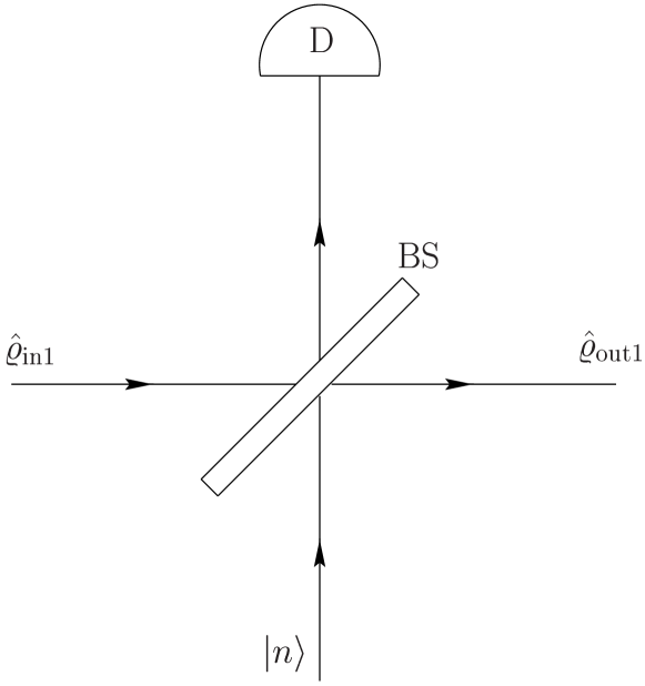
Figure 1: Scheme of the experimental setup. When a signal mode prepared in a state $\hat{\varrho}_{{\rm in}1}$ is mixed (beam splitter BS) with another input mode prepared in a Fock state $|n\rangle$ and in one of the output channels of the beam splitter $m$ photons are recorded (detector D), then the quantum state $\hat{\varrho}_{{\rm out}1}$ of the mode in the other output channel “collapses” to either a PSJP state ($n$ $\!<$ $\!m$) or a PAJP state ($n$ $\!>$ $\!m$).

An outline of the experimental setup is depicted in Figure 1. A field mode prepared in a state described by the density operator $\hat{\varrho}_{{\rm in}1}$ is mixed at a beam splitter with another mode prepared in a Fock state $|n\rangle$. The input-state density operator can then be written as

$$\hat{\varrho}_{\rm in}(n)=\hat{\varrho}_{{\rm in}1}\otimes|n\rangle_{2}\,{}_{2}\langle n|.$$ (11)

Using equations (6), (10) and (11), after some algebra the output-state density operator $\hat{\varrho}_{\rm out}$ $\!\equiv$ $\!\hat{\varrho}_{\rm out}(n)$ can be given by

$$\hat{\varrho}_{\rm out}(n)=\frac{1}{|T|^{2n}}\sum_{l=0}^{\infty}\sum_{m=0}^{\infty}\sum_{k=0}^{n}\sum_{j=0}^{n}(R^{*})^{m+j}R^{l+k}$$

$$\times\frac{(-1)^{l+m}}{\sqrt{k!j!m!l!}}\sqrt{\!{n\choose k}\!{n\choose j}\!{n\!-\!k\!+\!m\choose m}\!{n\!-\!j\!+\!l\choose l}}$$

$$\times\,T^{\hat{n}_{1}}{\hat{a}_{1}}^{m}({\hat{a}_{1}^{\dagger}})^{k}\hat{\varrho}_{{\rm in}1}\hat{a}_{1}^{j}({\hat{a}_{1}^{\dagger}})^{l}(T^{*})^{\hat{n}_{1}}\!\otimes\!|n\!-\!k\!+\!m\rangle_{2}\,{}_{2}\langle n\!-\!j\!+\!l|.$$

From equation (LABEL:1.05) we see that the output modes are highly correlated to each other in general. When the photon number of the mode in the second output channel is measured and $m$ photons are detected, then the mode in the first output channel is prepared in a quantum state whose density operator $\hat{\varrho}_{{\rm out}1}(n,m)$ reads as

$$\hat{\varrho}_{{\rm out}1}(n,m)=\frac{{}_{2}\langle m|\hat{\varrho}_{\rm out}(n)|m\rangle_{2}}{{\rm Tr}_{1}\{_{2}\langle m|\hat{\varrho}_{\rm out}(n)|m\rangle_{2}\}}\,.$$ (13)

The probability of such an event is given by

$$P(n,m)={\rm Tr}_{1}\{_{2}\langle m|\hat{\varrho}_{\rm out}{(n)}|m\rangle_{2}\}$$ (14)

$$=\,\frac{|R|^{-2\nu}n!}{|T|^{2m}m!}\sum_{j=\mu}^{n}\sum_{k=\mu}^{n}(-|R|^{2})^{(j+k)}{m\choose j\!-\!\nu}{m\choose k\!-\!\nu}$$

$$\hskip 8.61108pt\times\,\sum_{n=\delta}^{\infty}\frac{n!|T|^{2n}}{(n\!+\!\nu)!}{n\!+\!j\choose j}{n\!+\!k\choose k}\langle n|\hat{\varrho}_{{\rm in}1}|n\rangle,$$

where the abbreviations

$$\nu=n-m,\quad\mu=\max(0,\nu),\quad\delta=\mu-\nu$$ (15)

have been used. Let us now assume that the mode in the first input channel is prepared in a mixed state

$$\hat{\varrho}_{{\rm in}1}=\sum_{\Phi}\tilde{p}_{\Phi}\,|\Phi\rangle\langle\Phi|$$ (16)

($\sum_{\Phi}\tilde{p}_{\Phi}$ $\!=$ $\!1$, $0$ $\!\leq$ $\!\tilde{p}_{\Phi}$ $\!\leq$ $\!1$). Combining equations (LABEL:1.05) and (13) and using equation (16), we find that the mode in the first output channel is prepared in a state

$$\hat{\varrho}_{{\rm out}1}(n,m)=\sum_{\Phi}\tilde{p}_{\Phi}|\,\Psi_{n,m}\rangle\big{\langle}\Psi_{n,m}|,$$ (17)

where

$$|\Psi_{n,m}\rangle={\cal N}_{n,m}^{-1/2}\sum_{k=\mu}^{n}\frac{(-|R|^{2})^{k}}{(k\!-\!\nu)!}{n\choose k}\hat{a}_{1}^{k-\nu}(\hat{a}^{\dagger}_{1})^{k}T^{\hat{n}_{1}}|\Phi\rangle,$$ (18)

${\cal N}_{n,m}$ being the normalization constant,

$${\cal N}_{n,m}=\sum_{k=\mu}^{n}\sum_{j=\mu}^{n}\frac{(-|R|^{2})^{k+j}}{(k\!-\!\nu)!(j\!-\!\nu)!}{n\choose k}{n\choose j}$$ (19)

$$\hskip 21.52771pt\times\,\langle\Phi|(T^{\ast})^{\hat{n}_{1}}\hat{a}_{1}^{j}(\hat{a}^{\dagger}_{1})^{j-\nu}\hat{a}_{1}^{k-\nu}(\hat{a}^{\dagger}_{1})^{k}T^{\hat{n}_{1}}|\Phi\rangle.$$

3 Photon-subtracted and photon-added Jacobi polynomial states

The properties of the conditional output state essentially depend on whether photons are effectively subtracted ($n$ $\!<$ $\!m$) or added ($n$ $\!>$ $\!m$). To be more specific, from equation (18) we obtain for $n$ $\!<$ $\!m$ the output state

$$|\Psi_{n,m}\rangle\!=\!{\cal N}_{n,m}^{-1/2}\sum_{k=0}^{n}\frac{(-|R|^{2})^{k}}{(k\!+\!|\nu|)!}{n\choose k}\hat{a}^{|\nu|}\hat{a}^{k}(\hat{a}^{\dagger})^{k}T^{\hat{n}}|\Phi\rangle$$ (20)

$$\!=\!{\cal N}_{n,m}^{-1/2}\hat{a}^{|\nu|}\Bigg{\{}\sum_{k=0}^{n}\frac{(-|R|^{2})^{k}k!}{(k\!+\!|\nu|)!}{n\choose k}{\hat{n}\!+\!k\choose k}\Bigg{\}}T^{\hat{n}}|\Phi\rangle,\quad$$

where the notation

$$\hat{a}^{k}(\hat{a}^{\dagger})^{k}=(\hat{n}+1)(\hat{n}+2)\cdots(\hat{n}+k)=k!{\hat{n}\!+\!k\choose k}\quad$$ (21)

has been introduced ($\hat{n}$ $\!\equiv$ $\!\hat{n}_{1}$). For $n$ $\!>$ $\!m$ we derive [on using the relation $\hat{n}(\hat{a}^{\dagger})^{l}$ $\!=$ $\!(\hat{a}^{\dagger})^{l}$ $\!(\hat{n}$ $\!+$ $\!l)$]

$$|\Psi_{n,m}\rangle=\frac{n!(-|R|^{2})^{\nu}}{m!{\cal N}_{n,m}^{1/2}}$$ (22)

$$\hskip 8.61108pt\times\sum_{k=0}^{m}\frac{(-|R|^{2})^{k}}{(k\!+\!\nu)!}{m\choose k}\hat{a}^{k}(\hat{a}^{\dagger})^{k}(\hat{a}^{\dagger})^{\nu}T^{\hat{n}}|\Phi\rangle,$$

$$=\,\frac{(-|R|^{2})^{\nu}n!}{m!{\cal N}_{n,m}^{1/2}}(\hat{a}^{\dagger})^{\nu}$$

$$\hskip 8.61108pt\times\ \Bigg{\{}\sum_{k=0}^{m}\frac{(-|R|^{2})^{k}k!}{(k\!+\!\nu)!}{m\choose k}{\hat{n}\!+\!\nu\!+\!k\choose k}\Bigg{\}}T^{\hat{n}}|\Phi\rangle.\quad$$

From equations (20) and (22) it can be shown (Appendix A) that the conditional output state is of the form

$$|\Psi_{n,m}\rangle\sim\left\{\begin{array}[]{ll}\hat{a}^{|\nu|}\,{\rm P}_{n}^{(|\nu|,\hat{n}-m)}(2|T|^{2}\!-\!1)T^{\hat{n}}|\Phi\rangle&{\rm for}\ \nu\!<\!0,\\[12.91663pt] (\hat{a}^{\dagger})^{\nu}{\rm P}_{m}^{(\nu,\hat{n}-m)}(2|T|^{2}\!-\!1)T^{\hat{n}}|\Phi\rangle&{\rm for}\ \nu\!>\!0,\end{array}\right.\quad$$ (25)

where ${\rm P}_{l}^{(\alpha,\beta)}(z)$ is the Jacobi polynomial. The following procedure is seen to yield the conditional output states from a chosen input state $|\Phi\rangle$ $\!=$ $\!\sum_{k=0}^{\infty}\,c_{k}|k\rangle$. ($i$) Replace the Fock-expansion coefficients $c_{k}$ with $c^{\prime}_{k}$ $\!\sim$ $\!{\rm P}_{n-\mu}^{(|\nu|,k-m)}$ $\!(2|T|^{2}$ $\!-$ $\!1)$ $\!T^{k}c_{k}$ to obtain a state $|\Phi^{\prime}\rangle$. ($ii$) Subtract photons from the state $|\Phi^{\prime}\rangle$ by repeated application of the photon-destruction operator to it or add photons to state $|\Phi^{\prime}\rangle$ by repeated application of the photon-creation operator to it. In what follows we will refer to the states $|\Phi^{\prime}\rangle$ as Jacobi polynomial (JP) states (in analogy to Hermite polynomial and Laguerre polynomial states [58, 59]). Note that for typical classes of states the input state $|\Phi\rangle$ and the state $|\Psi\rangle$ $\!\sim$ $\!T^{\hat{n}}|\Phi\rangle$ belong to the same class of states [25]. We see that the conditional output states $|\Psi_{n,m}\rangle$ produced in the scheme can be regarded as photon-subtracted Jacobi polynomial (PSJP) states ($n$ $\!<$ $\!m$) and photon-added Jacobi polynomial (PAJP) states ($n$ $\!>$ $\!m$). It should be pointed out that the PSJP states and the PAJP states are essentially different from each other in general, because of $[\hat{a},\hat{a}^{\dagger}]$ $\!\neq$ $\!0$. Clearly, when the input state is a Fock state, $|\Phi\rangle$ $\!=$ $\!|k\rangle$, then the conditional output states are the Fock states $|k$ $\!+$ $\!n$ $\!-$ $\!m\rangle$. Let us mention that when $m$ $\!=$ $\!n$ (i.e., $\nu$ $\!=$ $\!0$), then

$$|\Psi_{n,n}\rangle={\cal N}_{n,n}^{-1/2}{\rm P}_{n}^{(0,\hat{n}-n)}(2|T|^{2}\!-\!1)T^{\hat{n}}|\Phi\rangle\,.$$ (26)

4 PSJP and PAJP coherent states

To treat the states in a unified way, let us return to equation (18) and first consider Glauber coherent input states

$$|\Phi\rangle\equiv|\beta\rangle=e^{-|\beta|^{2}/2}\sum_{k=0}^{\infty}\frac{\beta^{k}}{\sqrt{k!}}\,|k\rangle,$$ (27)

with $\beta$ $\!=$ $\!|\beta|e^{i\varphi_{\beta}}$. Equation (18) then reads

$$|\Psi_{n,m}\rangle=\frac{1}{\sqrt{{\cal N}^{\prime}_{n,m}}}\sum_{k=\mu}^{n}\frac{(-|R|^{2})^{k}}{(k-\nu)!}{n\choose k}\,\hat{a}^{k\!-\!\nu}(\hat{a}^{\dagger})^{k}|\beta^{\prime}\rangle,$$ (28)

where $\beta^{\prime}$ $\!=$ $\!T\beta$ and ${\cal N}^{\prime}_{n,m}$ $\!=$ $\!e^{|\beta^{\prime}R|^{2}}{\cal N}_{n,m}$. Applying standard operator ordering techniques [60], we may write

$$\hat{a}^{m}(\hat{a}^{\dagger})^{n}=\sum_{l=0}^{\min\{m,n\}}{m\choose l}\frac{n!}{(n-l)!}(\hat{a}^{\dagger})^{n-l}\hat{a}^{m-l},$$ (29)

and hence

$$|\Psi_{n,m}\rangle=\frac{{\beta^{\prime}}^{-\nu}}{\sqrt{{\cal N}^{\prime}_{n,m}}}\sum_{k=\mu}^{n}(-|R|^{2})^{k}{n\choose k}$$ (30)

$$\hskip 43.05542pt\times\,\sum_{l=\mu}^{k}\frac{1}{(k-\nu)!}{k\choose l}(\beta^{\prime}\hat{a}^{\dagger})^{l}|\beta^{\prime}\rangle,$$

from which the Fock-state expansion of $|\Psi_{n,m}\rangle$ can easily be obtained to be

$$|\Psi_{n,m}\rangle=\frac{e^{-|\beta^{\prime}|^{2}/2}}{\sqrt{{\cal N}^{\prime}_{n,m}}}\sum_{k=\mu}^{n}(-|R|^{2})^{k}{n\choose k}$$ (31)

$$\hskip 8.61108pt\times\,\,\sum_{l=\mu}^{k}{k\choose l}\frac{{\beta^{\prime}}^{(l-\nu)}}{(l-\nu)!}\sum_{p=0}^{\infty}\frac{(\beta^{\prime})^{p}}{p!}\sqrt{(p+l)!}\;|p+l\rangle\quad$$

(for the photon-number statistics, see Appendix B). Using the identities [61]

$$\sum_{l=0}^{n}\frac{x^{l}}{\Gamma(l+\nu)}{n\choose l}=\frac{n!}{\Gamma(n+\nu)}{\rm L}_{n}^{\nu-1}(-x)$$ (32)

and

$$\sum_{l=0}^{n}\frac{t^{l}}{\Gamma(\alpha\!+\!l\!+\!1)}\frac{{\rm L}_{l}^{\alpha}(x)}{(n\!-\!l)!}\!=\!\frac{(1+t)^{n}{\rm L}_{n}^{\alpha}\left[tx/(1\!+\!t)\right]}{\Gamma(\alpha\!+\!n\!+\!1)}$$ (33)

[${\rm L}_{n}^{\alpha}(z)$ is the associated (or generalized) Laguerre polynomial [61]], we may give equation (30) in the more compact form of

$$|\Psi_{n,m}\rangle=\frac{|T|^{2n}n!}{{\beta^{\prime}}^{\nu}\sqrt{{\cal N}^{\prime}_{n,m}}}\frac{\left[-|R|^{2}/|T|^{2}\right]^{\mu}}{(n+\delta)!}$$ (34)

$$\hskip 51.6665pt\times\,\,{\rm L}_{n-\mu}^{|\nu|}\!\left(\frac{|R|^{2}}{|T|^{2}}\beta^{\prime}\hat{a}^{\dagger}\right)(\beta^{\prime}\hat{a}^{\dagger})^{\mu}|\beta^{\prime}\rangle.$$

In a similar way it follows that

$${\cal N}^{\prime}_{n,m}=\frac{1}{|\beta^{\prime}|^{2\nu}}\sum_{k=\mu}^{n}\sum_{j=\mu}^{n}(-|R|^{2})^{k+j}{n\choose k}{n\choose j}$$ (35)

$$\hskip 25.83325pt\times\,\sum_{l=\mu}^{k}\sum_{l^{\prime}=\mu}^{j}{k\choose l}{j\choose l^{\prime}}\frac{{\beta^{\prime}}^{l}(\beta^{\prime\ast})^{l^{\prime}}\chi_{l^{\prime},l}^{(1)}(\beta^{\prime})}{(l-\nu))!(l^{\prime}-\nu)!}\,,$$

where

$$\chi_{l,k}^{(1)}(\alpha)=\left\{\begin{array}[]{ll}k!{\alpha}^{l-k}{\rm L}_{k}^{l-k}(-|\alpha|^{2})&{\rm for}\ l\geq k,\\[2.15277pt] l!(\alpha^{\ast})^{k-l}{\rm L}_{l}^{k-l}(-|\alpha|^{2})&{\rm for}\ l<k.\end{array}\right.$$ (38)

From equations (30) or (34) we find that PSJP and PAJP coherent states are finite superpositions of photon-added coherent states. In particular for $n$ $\!<$ $\!m$ equation (34) reduces to

$$|\Psi_{n,m}\rangle\sim{\rm L}_{n}^{|\nu|}\!\left(\frac{|R|^{2}}{|T|^{2}}\beta^{\prime}\hat{a}^{\dagger}\right)|\beta^{\prime}\rangle,$$ (39)

from which we see that when $|\beta^{\prime}|$ $\!\ll$ $\!1$ and $\gamma$ $\!=$ $\!(|R|^{2}/|T|^{2})\beta^{\prime}$ finite, then the PSJP state $|\Psi_{n,m}\rangle$ is (approximately) a superposition of $n$ Fock states, because of $|\beta^{\prime}\rangle$ $\!\approx$ $\!|0\rangle$.

The probability of producing PSJP and PAJP coherent states can be obtained from equation (14). After some calculation we derive (Appendix C)

$$P(n,m)=e^{-|R|^{2}|\beta^{2}|}\frac{|R|^{-2\nu}n!}{|T|^{2m}m!}$$ (40)

$$\times\,\sum_{k=\mu}^{n}\sum_{j=\mu}^{n}(-|R|^{2})^{k+j}{m\choose k\!-\!\nu}{m\choose j\!-\!\nu}\chi^{(2)}_{k,j}(\beta^{\prime},\nu),\quad$$

where

$$\chi_{k,j}^{(2)}(\alpha,\nu)=$$ (43)

$$\,\left\{\begin{array}[]{ll}\displaystyle\sum_{l=0}^{k}{k\choose l}\frac{(j-\nu)!)}{l!j!}{\rm L}_{j-\nu}^{l+|\nu|}(-|\alpha|^{2})|\alpha|^{2l}&{\rm for}\ \nu\geq 0,\\[17.22217pt] \displaystyle\sum_{l=0}^{k}{k\choose l}\frac{(j+l)!)}{l!j!}{\rm L}_{j+l}^{-l+|\nu|}(-|\alpha|^{2})|\alpha|^{2|\nu|}&{\rm for}\ \nu<0.\end{array}\right.\quad$$

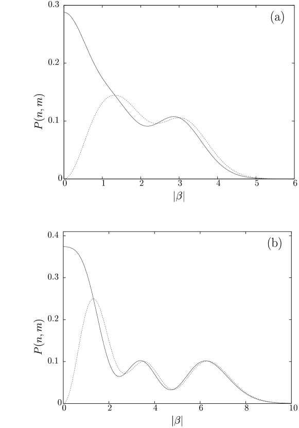
Figure 2: The probability of producing ($n$ $\!=$ $\!2$, $m$ $\!=$ $\!3$) PSJP coherent states (dashed line) and ($n$ $\!=$ $\!3$, $m$ $\!=$ $\!2$) PAJP coherent states (solid line) is shown as a function of $|\beta|$ for two values of the beam-splitter transmittance [(a) $|T|^{2}$ $\!=$ $\!0.4$; (b) $|T|^{2}$ $\!=$ $\!0.81$].

In Figure 2 examples of $P(n,m)$ are plotted for two absolute values of the beam-splitter transmittance. We see that $P(n,m)$ is an oscillating function of the absolute value of the coherent input amplitude, which is due to the interference of the incoming fields at the beam splitter. As expected, for $n$ $\!<$ $\!m$ the probability $P(n,m)$ goes to zero as the coherent amplitude does.

The superposition of photon-added coherent states, equation (30), gives rise to strong quantum interference, as it can be seen from the quadrature distribution

$$p_{n}(x,\varphi|m)=|\langle x,\varphi|\Psi_{n,m}\rangle|^{2}.$$ (44)

Using the Fock-state expansions (31) and [60]

$$|x,\varphi\rangle=(\pi)^{-1/4}e^{-x^{2}/2}\sum_{k=0}^{\infty}\frac{e^{ik\varphi}}{\sqrt{2^{k}k!}}\,{\rm H}_{k}(x)|k\rangle$$ (45)

[${\rm H}_{k}(x)$, Hermite polynomial] of the states $|\Psi_{n,m}\rangle$ and $|x,\varphi\rangle$, respectively, and recalling the identity [61]

$$\sum_{k=0}^{\infty}\frac{z^{k}}{k!}\,{\rm H}_{k+n}(x)=\,\exp\!\left(2xz-z^{2}\right){\rm H}_{n}(x-z),$$ (46)

we find that

$$p_{n}(x,\varphi|m)=\frac{|\beta^{\prime}|^{-2\nu}}{{\cal N}^{\prime}_{n,m}\sqrt{\pi}}$$ (47)

$$\times\exp\!\left\{\!-\!\left[x\!-\!\sqrt{2}|\beta^{\prime}|\cos(\varphi\!-\!\varphi_{\beta^{\prime}})\right]^{2}\right\}\Bigg{|}\sum_{k=\mu}^{n}(-|R|^{2})^{k}$$

$$\times{n\choose k}\sum_{l=\mu}^{k}{k\choose l}\frac{(2^{-\frac{1}{2}}{\beta^{\prime}}^{\ast}e^{i\varphi})^{l}}{(l-\nu)!}{\rm H}_{l}\!\left(x\!-\!2^{-\frac{1}{2}}{\beta^{\prime}}^{\ast}e^{i\varphi}\right)\Bigg{|}^{2}\!\!,\quad$$

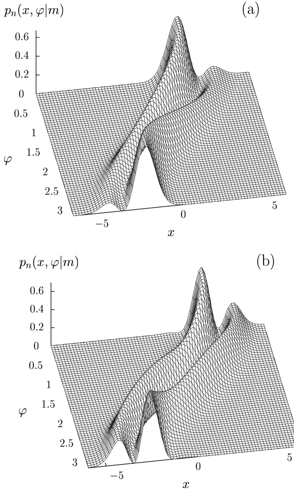
Figure 3: The quadrature-component distributions of (a) PSJP and (b) PAJP coherent states for $\beta^{\prime}$ $\!=$ $\!2.07$ ($|\beta|$ $\!=$ $\!2.3$, $|T|^{2}$ $\!=$ $\!0.81$) [(a) $n$ $\!=$ $\!2$, $m$ $\!=$ $\!3$, (b) $n$ $\!=$ $\!3$, $m$ $\!=$ $\!2$].

where $\varphi_{\beta^{\prime}}\!=\!\varphi_{\beta}+\varphi_{T}$. Examples of $p_{n}(x,\varphi|m)$ are plotted in Figure 3 for $\beta^{\prime}$ $\!=$ $\!2.07$ and (a) $n=2$, $m=3$ [$P(n,m)\approx 9.7\%$] and (b) $n=3$, $m=2$ [$P(n,m)\approx 6.7\%$]. From the figure it is clearly seen that the states are extremely non-Gaussian squeezed coherent states owing to quantum interference.

Next let us consider the Husimi function

$$Q_{n}(x,p|m)=\frac{1}{2\pi}\,|\langle\alpha|\Psi_{n,m}\rangle|^{2},$$ (48)

with $|\alpha\rangle$ being a coherent state and $\alpha$ $\!=$ $\!2^{-1/2}(x\!+\!ip)$. Expanding $|\alpha\rangle$ and $|\Psi_{n,m}\rangle$ in the Fock basis, on applying equations (27) and (31) respectively, we derive

$$Q_{n}(x,p|m)=\frac{\exp\!\left[-|\alpha\!-\!\beta^{\prime}|^{2}\right]}{2\pi|\beta^{\prime}|^{2\nu}{\cal N}^{\prime}_{n,m}}$$ (49)

$$\hskip 17.22217pt\times\left|\sum_{k=\mu}^{n}(-|R|^{2})^{k}{n\choose k}\sum_{l=\mu}^{k}{k\choose l}\frac{(\alpha{\beta^{\prime}}^{\ast})^{l}}{(l\!-\!\nu)!}\right|^{2}\!.$$

We again use the relations (32) and (33) and rewrite equation (49) as

$$Q_{n}(x,p|m)=\frac{|T|^{4n}(n!)^{2}}{2\pi{\cal N}^{\prime}_{n,m}|\beta^{\prime}|^{2\nu}}\frac{(-|RT\alpha\beta^{\prime}|)^{2\mu}}{(n+\delta)!}$$ (50)

$$\hskip 51.6665pt\times\,e^{-|\alpha-\beta^{\prime}|^{2}}\left|{\rm L}_{n-\mu}^{|\nu|}\!\left(\frac{|R|^{2}\alpha{\beta^{\prime}}^{\ast}}{|T|^{2}}\right)\right|^{2}\!.$$

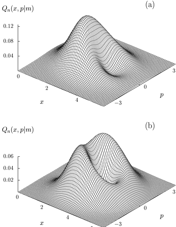
Figure 4: The Husimi function of (a) PSJP and (b) PAJP coherent states for $\beta^{\prime}$ $\!=$ $\!2.07$ ($|\beta|$ $\!=$ $\!2.3$, $|T|^{2}$ $\!=$ $\!0.81$) [(a) $n$ $\!=$ $\!2$, $m$ $\!=$ $\!3$, (b) $n$ $\!=$ $\!3$, $m$ $\!=$ $\!2$].

Figure 4 shows plots of the Husimi function for $\beta^{\prime}$ $\!=$ $\!2.07$ and (a) $n$ $\!=$ $\!2$, $m$ $\!=$ $\!3$ and (b) $n$ $\!=$ $\!3$, $m$ $\!=$ $\!2$. It should be pointed out that (the square root of) the difference between the height of the Husimi function and $1/(2\pi)$ can be regarded, in a sense, as a measure of the degree of nonclassicality [30, 62]. For the most classical states, i.e., for the Glauber coherent states and only for them, the Husimi function attains the maximum height of $1/(2\pi)\approx 0.16$. Thus from Figures 4(a) and 4(b) we see that the PSJP coherent state ($n$ $\!<$ $\!m$) is more classical than the PAJP coherent state ($n$ $\!>$ $\!m$) – a behaviour that is observed for a wide range of values of $|\beta^{\prime}|$.

Among the phase-space functions that have been shown to be inferable from measurable data, the Wigner function

$$W_{n}(x,p|m)=\frac{1}{\pi}\int\limits_{-\infty}^{+\infty}{d}y\,e^{2ipy}\langle x\!-\!y|\Psi_{n,m}\rangle\langle\Psi_{n,m}|x\!+\!y\rangle$$ (51)

($|x\rangle$ $\!=$ $\!|x,\varphi\rangle|_{\varphi=0}$) reflects quantum features most distinctly. In order to calculate it, we again use the Fock-state expansions (31) and (45) [together with equation (46)]. After some calculation we derive

$$W_{n}(x,p|m)=\hbox to0.0pt{$\displaystyle\frac{e^{-\left[\!x^{2}+{\textstyle\frac{1}{2}}\left(\beta^{\prime}\!+\!\beta^{\prime\ast}\right)^{2}\!-\sqrt{2}x(\beta^{\prime}\!+\!\beta^{\prime\ast})\right]}}{\pi{\cal N}^{\prime}_{n,m}|\beta^{\prime}|^{2\nu}}$\hss}$$ (52)

$$\times\,\sum_{k=\mu}^{n}\sum_{j=\mu}^{n}(-|R|^{2})^{k+j}{n\choose k}{n\choose j}\sum_{l=\mu}^{k}\sum_{l^{\prime}=\mu}^{j}{k\choose l}{j\choose l^{\prime}}$$

$$\times\,\frac{(2^{-1/2}\beta^{\prime})^{l}(2^{-1/2}{\beta^{\prime}}^{\ast})^{l^{\prime}}}{(l-\nu)!(l^{\prime}-\nu)!}\!\!\int\limits_{-\infty}^{+\infty}\!\!{d}y\,e^{-y^{2}+y[2ip+\sqrt{2}({\beta^{\prime}}^{\ast}-\beta^{\prime})]}$$

$$\times\,{\rm H}_{l}(x\!-\!y\!-\!2^{-1/2}\beta^{\prime}){\rm H}_{l^{\prime}}(x\!+\!y\!-\!2^{-1/2}{\beta^{\prime}}^{\ast}).$$

We then use the integral identity [61]

$$\int\limits_{-\infty}^{+\infty}{d}x\,e^{-x^{2}}{\rm H}_{m}(x\!+\!a){\rm H}_{n}(x\!+\!b)$$ (53)

$$\hskip 21.52771pt=\,\frac{\sqrt{\pi}2^{n}m!}{b^{m-n}}{\rm L}_{m}^{n-m}(-2ab)\quad(m\leq n),$$

and perform the $y$-integration to obtain

$$W_{n}(x,p|m)=\hbox to0.0pt{$\displaystyle\frac{e^{-|x+ip-\sqrt{2}\beta^{\prime}|^{2}}}{|\beta^{\prime}|^{2\nu}\pi{\cal N}^{\prime}_{n,m}}\sum_{k=\mu}^{n}\sum_{j=\mu}^{n}\bigg{\{}(-|R|^{2})^{k+j}$\hss}$$ (54)

$$\times\,{n\choose k}{n\choose j}\sum_{l=\mu}^{k}\sum_{l^{\prime}=\mu}^{j}{k\choose l}{j\choose l^{\prime}}\frac{(\beta^{\prime})^{l}(\beta^{\prime\ast})^{l^{\prime}}}{(l-\nu))!(l^{\prime}-\nu)!}$$

$$\hskip 8.61108pt\times\,\chi_{l^{\prime},l}^{(3)}\!\left[\sqrt{2}(x\!+\!ip\!-\!2^{-1/2}\beta^{\prime})\right]\bigg{\}},$$

where

$$\chi_{l,k}^{(3)}(\alpha)=\left\{\begin{array}[]{ll}(-1)^{k}k!{\alpha}^{l-k}{\rm L}_{k}^{l-k}(|\alpha|^{2})&{\rm for}\ l\geq k,\\[2.15277pt] (-1)^{l}l!(\alpha^{*})^{k-l}{\rm L}_{l}^{k-l}(|\alpha|^{2})&{\rm for}\ l<k.\end{array}\right.$$ (57)

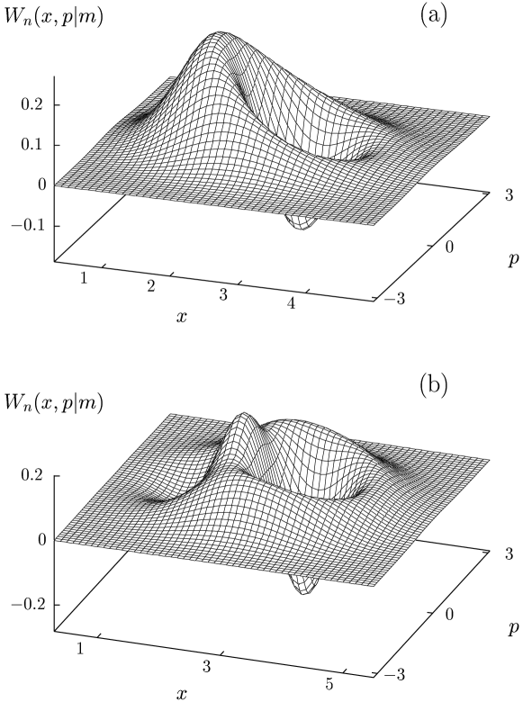
Figure 5: The Wigner function of (a) PSJP and (b) PAJP coherent states for $\beta^{\prime}$ $\!=$ $\!2.07$ ($|\beta|$ $\!=$ $\!2.3$, $|T|^{2}$ $\!=$ $\!0.81$) [(a) $n$ $\!=$ $\!2$, $m$ $\!=$ $\!3$, (b) $n$ $\!=$ $\!3$, $m$ $\!=$ $\!2$].

In Figure 5 plots of the Wigner function $W_{n}(x,p|m)$ are shown for $\beta^{\prime}$ $\!=$ $\!2.07$ and (a) $n$ $\!=$ $\!2$, $m$ $\!=$ $\!3$ and (b) $n$ $\!=$ $\!3$, $m$ $\!=$ $\!2$. We see that $W_{n}(x,p|m)$ for $n$ $\!>$ $m$ is more structurized owing to quantum interference and stronger negative than for $n$ $\!<$ $m$, which again reveals that the PAJP coherent state is more nonclassical than the PSJP coherent state.

5 PSJP and PAJP squeezed vacuum states

Let us briefly comment on PSJP and PAJP squeezed vacuum states that are realized when the input state is a squeezed vacuum $\hat{S}(\xi)|0\rangle$, with $\hat{S}(\xi)$ $\!=$ $\!\exp\{-\frac{1}{2}[\xi(\hat{a}^{\dagger})^{2}$ $\!-$ $\!\xi^{\ast}\hat{a}^{2}]\}$ being the squeeze operator. Hence we may write

$$|\Phi\rangle\equiv\hat{S}(\xi)|0\rangle=(1-|\kappa|^{2})^{\frac{1}{4}}\sum_{k=0}^{\infty}\frac{[(2k)!]^{1/2}}{2^{k}k!}\,\kappa^{k}|2k\rangle,$$ (58)

where the notation $\kappa$ $\!\equiv$ $\!\kappa(\xi)$ $\!=$ $\!-e^{i\varphi_{\xi}}\tanh|\xi|$ has been introduced ($\xi$ $\!=$ $\!|\xi|e^{i\varphi_{\xi}}$). According to equation(18), the conditional output states are then given by

$$|\Psi_{n,m}\rangle=\frac{1}{\sqrt{{\cal N}^{\prime}_{n,m}}}\sum_{k=\mu}^{n}\frac{(-|R|^{2})^{k}}{(k-\nu)!}{n\choose k}\hat{a}_{1}^{k-\nu}(\hat{a}^{\dagger}_{1})^{k}\hat{S}(\xi^{\prime})|0\rangle,$$ (59)

with ${\cal N}^{\prime}_{n,m}\!=\![(1-|\kappa^{\prime}|^{2})/(1-|\kappa|^{2})]^{1/2}\!{\cal N}_{n,m}$. In the photon-number basis $|\Psi_{n,m}\rangle$ reads as

$$|\Psi_{n,m}\rangle=\frac{(1-|\kappa^{\prime}|^{2})^{\frac{1}{4}}}{\sqrt{{\cal N}^{\prime}_{n,m}}}\sum_{k=\mu}^{n}\frac{(-|R|^{2})^{k}}{(k-\nu)!}{n\choose k}$$ (60)

$$\times\!\sum_{p=\mu}^{\infty}\frac{(p-\nu+k)!{\textstyle\frac{1}{2}}\!\left[1\!+\!(-1)^{p-\nu}\right]}{\Gamma\!\left[{\textstyle\frac{1}{2}}(p\!-\!\nu)\!+\!1\right]\sqrt{p!}}\left({\textstyle\frac{1}{2}}\kappa^{\prime}\right)^{(p-\nu)/2}|p\rangle,$$

with $\kappa^{\prime}$ $\!=$ $\!T^{2}\kappa$. From equation (60) we easily see that when the difference between the number $n$ of photons in the second input channel of the beam splitter and the number $m$ of photons detected in the second output channel, i.e., the parameter $\nu$ $\!=$ $\!n$ $\!-$ $\!m$, is even (odd), then the mode in the first output channel is prepared in a PSJP or PAJP squeezed vacuum state $|\Psi_{n,m}\rangle$ that contains only Fock states with even (odd) numbers of photons. Similarly to ordinary photon-subtracted and photon-added squeezed vacuum states [23, 24], it can be shown that the PSJP and PAJP squeezed vacuum states are Schrödinger-cat-like states. In particular, from equation (60) it can be found that $|\Psi_{n,m}\rangle$ can be given by a superposition of two mesoscopically distinguishable states,

$$|\Psi_{n,m}\rangle\sim|\Psi^{(+)}_{n,m}\rangle+|\Psi^{(-)}_{n,m}\rangle,$$ (61)

where

$$|\Psi^{(\pm)}_{n,m}\rangle=\frac{1}{\sqrt{{{\cal N}^{\prime(\pm)}_{n,m}}}}\sum_{p=\mu}^{\infty}C^{(\pm)}_{n,m,p}(\kappa^{\prime})\,|p\rangle,$$ (62)

with

$$C^{(\pm)}_{n,m,p}(\kappa^{\prime})=\sum_{k=\mu}^{n}\frac{(-|R|^{2})^{k}}{(k-\nu)!}{n\choose k}$$ (63)

$$\hskip 34.44434pt\times\,\frac{(p-\nu+k)!}{\Gamma\!\left[{\textstyle\frac{1}{2}}(p\!-\!\nu)\!+\!1\right]\sqrt{p!}}\left(\pm\sqrt{\textstyle\frac{1}{2}}\kappa^{\prime}\right)^{p-\nu}\!\!\!.\quad$$

A detailed analysis can be given in a way similar to that in [23, 24]. We therefore renounce the somewhat lengthy calculations here.

6 Relations to other states

From equation (25) and the property of the Jacobi polynomials that

$${\rm P}^{(\alpha,\beta)}_{l}(1)=(-1)^{l}{\rm P}^{(\alpha,\beta)}_{l}(-1)={{l\!+\!\alpha\choose l}}$$ (64)

we see that for sufficiently small values of $|T|$ ($|T|$ $\!\to$ $\!0$) or values of $|T|$ close to unity ($|T|$ $\!\to$ $\!1$) equation (25) approximately reduces to

$$|\Psi_{n,m}\rangle\sim\left\{\begin{array}[]{ll}\hat{a}^{|\nu|}T^{\hat{n}}|\Phi\rangle&{\rm for}\ \nu=n-m<0,\\[8.61108pt] (\hat{a}^{\dagger})^{\nu}T^{\hat{n}}|\Phi\rangle&{\rm for}\ \nu=n-m>0.\end{array}\right.$$ (67)

As expected, in these limiting cases the produced conditional states $|\Psi_{n,m}\rangle$ reduce to ordinary photon-subtracted ($\nu$ $\!<$ $\!0$) or photon-added ($\nu$ $\!>$ $\!0$) states.

Further, equation (25) reveals that when the second input mode is in the vacuum state and in the second output channels a nonvanishing number of photons is detected ($n$ $\!=$ $\!0$, $m$ $\!>$ $\!0$), then usual photon subtraction is observed,

$$|\Psi_{0,m}\rangle=(1/m!){\cal N}_{0,m}^{-1/2}\,\hat{a}^{m}T^{\hat{n}}|\Phi\rangle,$$ (68)

independently of the value of $T$. Similarly, when a Fock state $|n\rangle$ is fed into the second input channel and a zero-photon conditional measurement is performed in the second output channel ($n$ $\!>$ $\!0$, $m$ $\!=$ $\!0$), then the mode in the first output channel is prepared in an ordinary photon-added state

$$|\Psi_{n,0}\rangle=(-|R|^{2})^{n}{\cal N}_{n,0}^{-1/2}\,(\hat{a}^{\dagger})^{n}\,T^{\hat{n}}|\Phi\rangle.$$ (69)

Photon-subtracted states and photon-added states of the type given in equations (68) and (69), respectively, have been studied by several authors [23, 24, 25, 26, 27, 28, 29, 30].

6.1 Displaced Fock states

Since the coherent states $|\beta\rangle$ $\!=$ $\!\hat{D}(\beta)|0\rangle$ [$\hat{D}(\beta)$ $\!=\!$ $\!\exp(\beta\hat{a}^{\dagger}$ $\!-$ $\!\beta^{\ast}\hat{a})$] are the eigenstates to the destruction operator ($\hat{a}|\beta\rangle$ $\!=$ $\!\beta|\beta\rangle$), it is obvious that subtracting photons from a coherent state yields again a coherent state. Photon-added coherent states are highly nonclassical states. From

$$(\hat{a}^{\dagger})^{n}|\beta\rangle = (\hat{a}^{\dagger})^{n}\hat{D}(\beta)|0\rangle$$ (70)

$$= \hat{D}(\beta)\hat{D}^{\dagger}(\beta)(\hat{a}^{\dagger})^{n}\hat{D}(\beta)|0\rangle,$$

we find that

$$(\hat{a}^{\dagger})^{n}|\beta\rangle = \hat{D}(\beta)(\hat{a}^{\dagger}+\beta^{\ast})^{n}|0\rangle$$ (71)

$$= \sum_{k=0}^{n}{n\choose k}\sqrt{k!}\,(\beta^{\ast})^{n-k}\hat{D}(\beta)|k\rangle.$$

Equation (71) reveals that photon-added coherent states are finite superpositions of displaced Fock states $\hat{D}(\beta)|n\rangle$ [28] (for the properties of displaced Fock states, see [2, 3, 4]. From equations (30) and (34) we know that PSJP and PAJP coherent states can be given by finite superpositions of photon-added coherent states. Expressing the latter, according to equations (70) and (71), in terms of displaced Fock states, we see that PSJP and PAJP states are also finite superpositions of displaced Fock states.

Similarly, displaced Fock states can be given by finite superpositions of photon-added coherent states. To show this, we write

$$\hat{D}(\beta)|n\rangle = \hat{D}(\beta)\frac{1}{\sqrt{n!}}\,(\hat{a}^{\dagger})^{n}|0\rangle$$ (72)

$$= \frac{1}{\sqrt{n!}}\hat{D}(\beta)(\hat{a}^{\dagger})^{n}\hat{D}^{\dagger}(\beta)\hat{D}(\beta)|0\rangle,$$

and hence

$$\hat{D}(\beta)|n\rangle = \frac{1}{\sqrt{n!}}(\hat{a}^{\dagger}-\beta^{\ast})^{n}|\beta\rangle$$ (73)

$$= \frac{1}{\sqrt{n!}}\sum_{l=0}^{n}{n\choose l}(-\beta^{\ast})^{n-l}(\hat{a}^{\dagger})^{l}|\beta\rangle.$$

Note that from equation (73) and equation (34) for $|T|^{2}$ $\!=$ $\!|R|^{2}$ $\!=$ $\!0.5$ and $\beta$ $\!\approx$ $\!1$ it follows that $|\Psi_{11}\rangle$ $\!\sim$ $\!\hat{D}(\beta)|n\rangle|_{n=1}$, i.e., the conditional measurement schemes realizes a coherently displaced single-photon Fock state.

6.2 Near-photon-number eigenstates

Near-photon-number eigenstates are an example of minimum uncertainty states that are defined by the eigenstates of the operator $\hat{Y}$ $\!=$ $\!\hat{n}$ $\!-$ $\!i|\beta|\hat{x}(\varphi)$, which is associated with the “simultaneous” measurement of photon number and quadrature components [8]. The states are also called crescent states and have been studied in a number of papers [8, 9, 10, 11, 12, 13]. In particular, they can be expressed in the form of

$$|\psi\rangle\sim(\hat{a}^{\dagger}+\beta^{\ast})^{n}|\beta\rangle,$$ (74)

or alternatively, in terms of nonunitarily shifted Fock states, and it was shown that they can be generated by state reduction via photon-number conditional measurement in nondegenerate parametric down conversion [13].

From equation (74) it is easily seen that

$$|\psi\rangle\sim\hat{D}^{\dagger}(\beta)(\hat{a}^{\dagger})^{n}\hat{D}(\beta)|\beta\rangle=\hat{D}(-\beta)(\hat{a}^{\dagger})^{n}|2\beta\rangle.$$ (75)

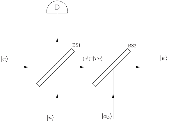
Figure 6: Experimental setup for preparing near-photon-number states (crescent states). A mode prepared in a coherent state $|\alpha\rangle$ is first mixed (beam splitter BS1) with a mode prepared in a Fock state $|n\rangle$ and a zero-photon output measurement is performed (detector D). The output mode prepared in a photon-added coherent state $(\hat{a}^{\dagger})^{n}|2\beta\rangle$ ($2\beta$ $\!=$ $\!T\alpha$) is then mixed (beam splitter BS2 with transmittance $\tilde{T}$ close to unity) with a mode prepared in a strong coherent state $|\alpha_{L}\rangle$ such that $\beta$ $\!=$ $\!-(\tilde{R}/\tilde{T})\alpha_{L}$.

Equation (75) reveals that near-photon-number eigenstates are coherently displaced photon-added coherent states, which offers the possibility of producing them by conditional measurement on a beam splitter and subsequent coherent displacement. As it is depicted in Figure 6, a mode prepared in a coherent state $|\alpha\rangle$ is first mixed with a mode prepared in a Fock state $|n\rangle$, and a zero-photon measurement is performed in one output channel of the beam splitter to prepare the mode in the other output channel in a photon-added coherent state $(\hat{a}^{\dagger})^{n}|2\beta\rangle$ ($2\beta$ $\!=$ $\!T\alpha$). To realize the coherent displacement $\hat{D}(-\beta)$, this mode and a strong local-oscillator mode prepared in state $|\alpha_{L}\rangle$ are then superimposed by another, unbalanced beam splitter of high transmittance $\tilde{T}$ and low reflectance $\tilde{R}$ such that $\beta$ $\!=$ $\!-(\tilde{R}/\tilde{T})\alpha_{L}$.

6.3 Squeezed Fock states

Next let us consider a photon-added squeezed vacuum state,

$$(\hat{a}^{\dagger})^{n}\hat{S}(\xi)|0\rangle = \hat{S}(\xi)\hat{S}^{\dagger}(\xi)(\hat{a}^{\dagger})^{n}\hat{S}(\xi)|0\rangle$$ (76)

$$= (1-|\kappa|^{2})^{-n/2}\hat{S}(\xi)(\hat{a}^{\dagger}+\kappa^{\ast}\hat{a})^{n}|0\rangle\quad$$

[$\hat{S}(\xi)$ $\!=$ $\!\exp\{-\frac{1}{2}[\xi(\hat{a}^{\dagger})^{2}$ $\!-$ $\!\xi^{\ast}\hat{a}^{2}]\}$, $\kappa$ $\!\equiv$ $\!\kappa(\xi)$ $\!=$ $\!-e^{i\varphi_{\xi}}\tanh|\xi|$, $\xi$ $\!=$ $\!|\xi|e^{i\varphi_{\xi}}$]. Using standard ordering techniques for boson operators [60], we derive

$$(\hat{a}^{\dagger}+\epsilon\hat{a})^{n}=\sum_{l=0}^{n}{n\choose l}(\epsilon)^{n-l}$$ (77)

$$\hskip 12.91663pt\times\,\sum_{k=0}^{[\frac{l}{2}]}\frac{(2\epsilon)^{k}}{\sqrt{\pi}}{l\choose 2k}\Gamma\!\left(k+{\textstyle\frac{1}{2}}\right)(\hat{a}^{\dagger})^{l-2k}\hat{a}^{n-l},$$

which enables us to rewrite equation (76) as

$$(\hat{a}^{\dagger})^{n}\hat{S}(\xi)|0\rangle=(1-|\kappa|^{2})^{-n/2}$$ (78)

$$\hskip 43.05542pt\times\,\sum_{k=0}^{[\frac{n}{2}]}\frac{n!(\kappa^{\ast})^{k}}{2^{k}k!\sqrt{(n\!-\!2k)!}}\,\hat{S}(\xi)|n-2k\rangle.$$

Analogously, for the photon-subtracted squeezed vacuum states we find that

$$\hat{a}^{m}\hat{S}(\xi)|0\rangle = \hat{S}(\xi)\hat{S}^{\dagger}(\xi)\hat{a}^{m}\hat{S}(\xi)|0\rangle$$ (79)

$$= \kappa(1-|\kappa|^{2})^{-m/2}\hat{S}(\xi)(\hat{a}^{\dagger}+\kappa^{-1}\hat{a})^{m}|0\rangle\,,\qquad$$

and hence

$$\hat{a}^{m}\hat{S}(\xi)|0\rangle=\kappa(1-|\kappa|^{2})^{-m/2}$$ (80)

$$\hskip 43.05542pt\times\,\sum_{k=0}^{[\frac{m}{2}]}\frac{m!\left(1/\kappa\right)^{k}}{2^{k}k!\sqrt{(m-2k)!}}\,\hat{S}(\xi)|m-2k\rangle.\quad$$

Equations (78) and (80) show that photon-added and photon-subtracted squeezed vacuum states can be given by finite superpositions of squeezed Fock states $\hat{S}(\xi)|k\rangle$, and it is worth noting that the two classes of states realize two classes of Schrödinger-cat states [23, 25]. The extension of equations (78) and (80) to photon-added squeezed coherent states $(\hat{a}^{\dagger})^{n}\hat{D}(\beta)\hat{S}(\xi)|0\rangle$ and photon-subtracted squeezed coherent states $\hat{a}^{m}\hat{D}(\beta)\hat{S}(\xi)|0\rangle$ is straightforward. These two classes of states can be given by finite superpositions of displaced squeezed Fock states $\hat{D}(\beta)\hat{S}(\xi)|k\rangle$ (for the properties of displaced squeezed Fock states, see [5, 6]).

Displaced squeezed Fock states $\hat{D}(\beta)\hat{S}(\xi)|n\rangle$ can be rewritten as

$$\hat{D}(\beta)\hat{S}(\xi)|n\rangle=(n!)^{-1/2}\hat{D}(\beta)\hat{S}(\xi)(\hat{a}^{\dagger})^{n}|0\rangle$$ (81)

$$\hskip 8.61108pt=\,(n!)^{-1/2}\hat{D}(\beta)\hat{S}(\xi)(\hat{a}^{\dagger})^{n}\hat{S}^{\dagger}(\xi)\hat{S}(\xi)|0\rangle$$

$$\hskip 8.61108pt=\,[(1-|\kappa|^{2})^{n}n!]^{-1/2}\hat{D}(\beta)(\hat{a}^{\dagger}-\kappa^{\ast}\hat{a})^{n}\hat{S}(\xi)|0\rangle.\quad$$

From equations (81) and (77) it is seen that displaced squeezed Fock states cannot be given by finite superpositions of the photon-added squeezed states in general. Note that the displaced Fock states $\hat{D}(\beta)|k\rangle$ are finite superpositions of photon-added coherent states [see equation (73)].

6.4 Squeezed-state excitations

Squeezed-state excitations

$$|\beta,n;\xi\rangle\sim\hat{D}(\beta)(\hat{a}^{\dagger}+\kappa^{\ast}\hat{a})^{n}\hat{S}(\xi)|0\rangle$$ (82)

were introduced for diagonalizing the complete Gaussian class of phase-space functions [19, 20]. Note that although equation (82) formally resembles equation (81), squeezed-state excitations are quite different from displaced squeezed Fock states in general. It can be easily seen that

$$|\beta,n;\xi\rangle \sim \hat{D}(\beta)\hat{S}^{\dagger}(\xi)\hat{S}(\xi)(\hat{a}^{\dagger}+\kappa^{\ast}\hat{a})^{n}\hat{S}^{\dagger}(\xi)\hat{S}(2\xi)|0\rangle$$ (83)

$$\sim \hat{D}(\beta)\hat{S}^{\dagger}(\xi)(\hat{a}^{\dagger})^{n}\hat{S}(2\xi)|0\rangle$$

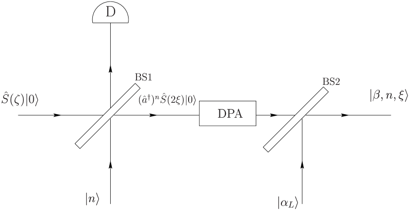
Figure 7: Experimental setup for preparing squeezed-state excitations. A mode prepared in a squeezed vacuum state $\hat{S}(\zeta)|0\rangle$ is first mixed (beam splitter BS1) with a mode prepared in a Fock state $|n\rangle$ and a zero-photon output measurement is performed (detector D), so that the output mode is prepared in a photon-added squeezed vacuum state $(\hat{a}^{\dagger})^{n}\hat{S}(2\xi|0\rangle$ [$\kappa(2\xi)$ $\!=$ $\!T^{2}\kappa(\zeta)$], which is then squeezed, e.g., by a degenerate parametric amplifier (DPA) to realize the squeezing parameter $-\xi$. Finally the so squeezed output mode is mixed (beam splitter BS2 with transmittance $\tilde{T}$ close to unity) with a mode prepared in a strong coherent state $|\alpha_{L}\rangle$ such that $\beta$ $\!=$ $\!(\tilde{R}/\tilde{T})\alpha_{L}$.

[cf. equation (76)]. We see that squeezed-state excitations are nothing but squeezed and subsequently displaced photon-added squeezed vacuum states, which implies the scheme in Figure 7 for producing them. Using a beam splitter, a mode prepared in a squeezed vacuum $\hat{S}(\zeta)|0\rangle$ is first mixed with a mode prepared in a Fock state $|n\rangle$ and a zero-photon measurement is performed in one output channel of the beam splitter to prepare the mode in the other output channel in a photon-added squeezed vacuum state $(\hat{a}^{\dagger})^{n}\hat{S}(2\xi)|0\rangle$ [$\kappa(2\xi)$ $\!=$ $\!T^{2}\kappa(\zeta)$]. This state is then squeezed (with $-\xi$ as squeezing parameter), e.g., by degenerate parametric amplification or by state reduction via quadrature-component conditional measurement in nondegenerate parametric down conversion [34]. Superimposing the outgoing mode and a strong local oscillator by an unbalanced beam splitter, the coherent displacement can be realized [$\beta$ $\!=$ $\!(\tilde{R}/\tilde{T})\alpha_{L}$; cf. Section 6.2].

7 Realistic experimental conditions

Let us first address the problem of realistic photon detection. Unfortunately, there are no highly efficient and precisely discriminating photodetectors available at present. To overcome this difficulty, photon chopping [63] was suggested for measuring the photon-number statistics. Let us remember that in such a scheme the mode to be detected is fed into an input channel of an optical $2N$-port array of beam splitters, the other $N$ $\!-$ $\!1$ input ports being unused. Highly efficient avalanche photodiodes in the $N$ output channels are used in order to record the coincidence event statistics. Since they only distinguish between photons being present or absent, the probability of obtaining $k$ clicks when $m$ photon are present is given by [63]

$$\tilde{P}_{N,\eta}(k|m)=\sum_{l}\tilde{P}_{N}(k|l)\,M_{l,m}(\eta)$$ (84)

($\eta$ is the detection efficiency), where

$$\tilde{P}_{N}(k|m)=\frac{1}{N^{m}}{N\choose k}\sum_{l=0}^{k}(-1)^{l}{k\choose l}(k-l)^{m}$$ (85)

for $k$ $\!\leq$ $\!m$, and $\tilde{P}_{N}(k|m)$ $\!=$ $\!0$ for $k$ $\!>$ $\!m$. The matrix

$${M}_{l,m}(\eta)={m\choose l}\eta^{l}(1-\eta)^{m-l}$$ (86)

for $l$ $\!\leq$ $\!m$, and ${M}_{l,m}(\eta)$ $\!=$ $\!0$ for $l$ $\!>$ $\!m$ represents the effect of nonperfect detection. Since detection of $k$ coincident events can result from various numbers $m$ of photons, the conditional state is in general a statistical mixture. Therefore in place of equation (17) we now have

$$\hat{\varrho}_{\rm out}(n,k)=\sum_{m,\Phi}\tilde{p}_{\Phi}P_{N,\eta}(n,m|k)\,|\Psi_{n,m}\rangle\langle\Psi_{n,m}|,$$ (87)

where $|\Psi_{n,m}\rangle$ is given in equation (18), and $P_{N,\eta}(n,m|k)$ is the probability of $m$ photons being present under the condition that $k$ coincidences are recorded. The conditional probability $P_{N,\eta}(n,m|k)$ can be obtained using the Bayes rule as

$$P_{N,\eta}(n,m|k)=\frac{1}{\tilde{P}_{N,\eta}(n,k)}\tilde{P}_{N,\eta}(k|m)\ P(n,m).$$ (88)

Here $P(n,m)$ is the prior probability (14) of $m$ photons being present, and accordingly, $\tilde{P}_{N,\eta}(n,k)$ is the prior probability of recording $k$ coincident events,

$$\tilde{P}_{N,\eta}(n,k)=\sum_{m}\tilde{P}_{N,\eta}(k|m)\ P(n,m).$$ (89)

Second, preparation of the reference mode in a Fock state is a nontrivial problem (for a review, see [1]; for single-photon Fock states, see also [64, 65, 66]; for multiphoton Fock states, see also [67, 68, 69, 70, 71]). In particular, a method for synthesizing multiphoton Fock states from single-photon Fock states (produced, e.g., in parametric down conversion) has been proposed [70, 71]. In the scheme, modes prepared in single-photon Fock states are fed into the input ports of an array of beam splitters and detectors survey all but one output port so that the mode in the free output port is prepared in the sought photon-number state. In practice however, it may be more realistic to consider statistical mixtures of photon-number states rather than pure Fock states. Let us return to equation (11) and assume that

$$\hat{\varrho}_{\rm in}=\hat{\varrho}_{{\rm in}1}\otimes\hat{\varrho}_{{\rm in}2},$$ (90)

where

$$\hat{\varrho}_{{\rm in}2}=\sum_{n}\tilde{p}_{n}\,|n\rangle\langle n|\,.$$ (91)

To be more specific, let us consider (as an example of a sub-Poissonian distribution) a binomial probability distribution,

$$\tilde{p}_{n}={n_{0}\choose n}p^{n}(1-p)^{n_{0}-n}\quad{\rm if}\quad n\leq n_{0}$$ (92)

and $\tilde{p}_{n}$ $\!=$ $\!0$ elsewhere ($0$ $\!<$ $\!p$ $\!<$ $\!1$). Note that for $p$ $\!\to$ $\!0$, $n_{0}$ $\!\to$ $\!\infty$, and $pn_{0}$ finite the binomial distribution (92) reduces to a Poisson distribution, with $\bar{n}$ $\!=$ $\!pn_{0}$ being the mean photon number. Using equations (90) and (91), from equation (87) we easily find that after recording $k$ coincident events the conditional mixed state now reads

$$\hat{\varrho}_{{\rm out}1}(k)=\sum_{n}\tilde{p}_{n}\,\hat{\varrho}_{{\rm out}1}(n,k)$$ (93)

$$\hskip 34.44434pt=\,\sum_{n,m,\Phi}\tilde{p}_{n}\tilde{p}_{\Phi}\,P_{N,\eta}(n,m|k)\Psi_{n,m}\rangle\big{\langle}\Psi_{n,m}|.\quad$$

Accordingly, the probability of detecting the state is the average of $P_{N,\eta}(n,k)$ given in equation (89), i.e.,

$$P_{N,\eta}(k) = \sum_{n}\tilde{p}_{n}P_{N,\eta}(n,k)$$ (94)

$$= \sum_{n,m}\tilde{p}_{n}\tilde{P}_{N,\eta}(k|m)P(n,m).$$ (95)

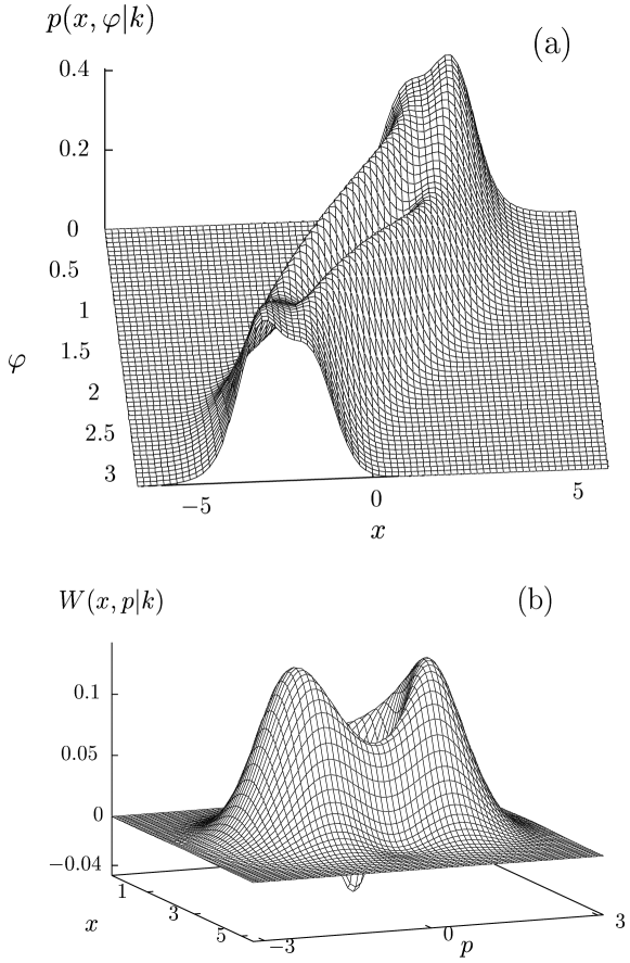
Figure 8: The quadrature-component distribution (a) and the Wigner function (b) of a mixed conditional output state (93) for a coherent input state with $\beta^{\prime}$ $\!=$ $\!2.07$ ($|\beta|$ $\!=$ $\!2.3$, $|T|^{2}$ $\!=$ $\!0.81$). The parameters of the photon-chopping detection scheme are $k$ $\!=$ $\!4$, $N$ $\!=$ $\!20$, $\eta$ $\!=$ $\!90$% and those of the input Fock-state mixture (91) are $n_{0}$ $\!=$ $\!4$ and $p$ $\!=$ $\!0.95$.

The quadrature-component distributions and the Wigner function of a mixed conditional output state (93) are plotted in figure 8 [$P_{N,\eta}(k)$ $\!\approx$ $\!21.4\%$]. We see that the quantum interference is still preserved for realistic values of the number of photodiodes and efficiencies ($k$ $\!=$ $\!4$, $N$ $\!=$ $\!20$, $\eta$ $\!=$ $\!90$%) and for a sub-Poissonian statistics of the input Fock-state mixture (91) [$\bar{n}$ $\!=$ $\!3.8$, $\overline{(\Delta n)^{2}}$ $\!=$ $\!0.19$].

8 Summary and conclusions

We have extended previous work on quantum-state preparation via conditional output measurement on a beam splitter and shown that when a mode prepared in a state $|\Phi\rangle$ is mixed with a mode prepared in an $n$-photon Fock state and $m$ photons are detected in one of the output channels of the beam splitter, then the mode in the other output channel is prepared in a photon-subtracted ($n$ $\!<$ $\!m$) or a photon-added ($n$ $\!>$ $\!m$) Jacobi polynomial state which is obtained by applying an operator-valued Jacobi polynomial to the state $|\Psi\rangle$ $\!\sim$ $T^{\hat{n}}|\Phi\rangle$. Since for typical classes of input states, such as thermal states, coherent states and squeezed states, the states $|\Phi\rangle$ and $|\Psi\rangle$ belong to the same class of states, the Jacobi polynomial states derived from $|\Phi\rangle$ and $|\Psi\rangle$ also belong to the same class of states. Jacobi polynomial states are nonclassical states in general, so that subtracting photons from or adding photons to them again yields nonclassical states in general.

The analysis has shown that PSJP and PAJP coherent states can be regarded as extremely non-Gaussian squeezed states. A characteristic feature of PSJP and PAJP squeezed vacuum states are the well pronounced quantum interferences associated with the quadrature-component noise reduction. Moreover, these two classes of states represent Schrödinger-cat-like states. Photon-added Jacobi polynomial states are more nonclassical than photon-subtracted Jacobi polynomial states in general. In particular when $n$ $\!=$ $\!0$ ($m$ $\!>$ $\!0$) or $m$ $\!=$ $\!0$ ($n$ $\!>$ $\!0$), respectively, then the states reduce to ordinary photon-subtracted or photon-added states. Whereas photon-added coherent states are non-Gaussian squeezed states, subtracting photons from a coherent state obviously leaves the state unchanged.

The analysis has further shown that there are close relations to other nonclassical states that have widely been studied. Hence combining state preparation via conditional output measurement on a beam splitter with other schemes offers novel possibilities of nonclassical-state generation and manipulation, such as the generation of near-photon-number eigenstates and squeezed-state excitations. Since near-photon-number eigenstates are coherently displaced photon-added coherent states, they can be generated by combining the scheme for photon adding with a scheme for coherently displacing a state. The latter can be realized by using a second beam splitter whose transmittance is close to unity and which mixes the mode prepared in a photon-added coherent state with a mode prepared in a strong coherent state. Similarly, a squeezed-state excitation can be prepared by appropriately squeezing a photon-added squeezed vacuum state followed by a coherent displacement of the state.

In order to demonstrate the feasibility of generating PSJP and PAJP states, we have calculated the corresponding event probabilities. Further, we have also allowed for both nonprecise input Fock-state preparation and nonprecise output photon counting. For this purpose we have considered sub-Poissonian mixtures of Fock states in place of pure Fock states and assumed that photon-chopping is adopted for photon counting. The results show that, apart from some smearing, typical properties of the states can still be observed even under realistic experimental conditions.

Appendix Appendix A: Proof of equation (25)

To prove equation (25), let us consider the operator function

$${\rm F}_{l}^{\mu}(\hat{n},|\nu|;T)=T^{\hat{n}}\sum_{k=0}^{l}\frac{(-|R|^{2})^{k}k!}{(k\!+\!|\nu|)!}{l\choose k}{\hat{n}\!+\!\mu\!+\!k\choose k},$$ (A.1)

which reads in the Fock basis as

$${\rm F}_{l}^{\mu}(\hat{n},|\nu|;T)=\sum_{n=0}^{\infty}\frac{T^{n}}{(n\!+\!\mu)!}$$ (A.2)

$$\hskip 8.61108pt\times\,\sum_{k=0}^{l}\frac{\Gamma(n\!+\!\mu\!+\!k\!+\!1)(-|R|^{2})^{k}}{\Gamma(k\!+\!|\nu|\!+\!1)}{l\choose k}|n\rangle\langle n|.$$

Introducing the integral representation of the gamma function $\Gamma(n$ $\!+$ $\!\mu$ $\!+$ $\!k$ $\!+$ $\!1)$, we have

$${\rm F}_{l}^{\mu}(\hat{n},|\nu|;T)=\sum_{n=0}^{\infty}\frac{T^{n}}{(n\!+\!\mu)!}\int_{0}^{\infty}\!dt\,t^{n+\mu}e^{-t}$$ (A.3)

$$\hskip 38.74988pt\times\,\sum_{k=0}^{l}\frac{(-|R|^{2}t)^{k}}{\Gamma(k\!+\!|\nu|\!+\!1)}{l\choose k}|n\rangle\langle n|.$$

We now use the sum rule (32) and the integral identity[61]

$$\int_{0}^{\infty}dt\,t^{\alpha-1}e^{-t}{\rm L}_{n}^{\beta}(ct)$$ (A.4)

$$\hskip 8.61108pt=\,\Gamma(\alpha){\rm P}_{n}^{(\beta,\alpha-\beta-n-1)}(1-2c)\quad({\rm Re}\ \alpha>0)\qquad$$

and obtain ($|R|^{2}$ $\!=$ $\!1$ $\!-$ $\!|T|^{2}$)

$${\rm F}_{l}^{\mu}(\hat{n},|\nu|;T)$$ (A.5)

$$\hskip 4.30554pt=\,\frac{l!}{(l\!+\!|\nu|)!}\sum_{n=0}^{\infty}{\rm P}_{l}^{(|\nu|,n+\mu-|\nu|-l)}\!\left(2|T|^{2}\!-\!1\right)T^{n}|n\rangle\langle n|$$

$$\hskip 4.30554pt=\,\frac{l!}{(l\!+\!|\nu|)!}{\rm P}_{l}^{(|\nu|,\hat{n}+\mu-|\nu|-l)}\!\left(2|T|^{2}-1\right)T^{\hat{n}}.$$

Combining equations (20), (22), (A.1) and (A.5) eventually yields equation (25).

Appendix Appendix B: Photon statistics of PSJP and PAJP coherent states

From equation (31) the photon-number distribution $p_{n,m}(l)$ $\!=$ $\!|\langle\,l|\Psi_{n,m}\rangle|^{2}$ of PSJP and PAJP coherent states can be given by

$$p_{n,m}(l)=\frac{e^{-|\beta^{\prime}|^{2}}l!|\beta^{\prime}|^{2l}}{{\cal N}^{\prime}_{n,m}|\beta^{\prime}|^{2\nu}}\Bigg{|}\sum_{k=\mu}^{n}(-|R|^{2})^{k}{n\choose k}$$ (B.1)

$$\hskip 68.88867pt\times\,\sum_{j=\mu}^{k}{k\choose j}\frac{\theta(l-j)}{(j\!-\!\nu)!(l\!-\!j)!}\Bigg{|}^{2},$$

where $\theta(n)$ $\!=$ $\!1$ for $n$ $\!\geq$ $\!0$ and $\theta(n)$ $\!=$ $\!0$ elsewhere. Further, from equations (28) and (29) it can be shown that the antinormally ordered moments of the photon number can by given by

$$\langle\Psi_{n,m}|\hat{a}^{p}(\hat{a}^{\dagger})^{p}|\Psi_{n,m}\rangle=\frac{|\beta^{\prime}|^{-2\nu}}{{\cal N}^{\prime}_{n,m}}\sum_{k=\mu}^{n}\sum_{j=\mu}^{n}(-|R|^{2})^{k+j}$$ (B.2)

$$\times{n\choose k}\!{n\choose j}\!\sum_{l=\mu}^{k}\sum_{l^{\prime}=\mu}^{j}\!{k\choose l}\!{j\choose l^{\prime}}\frac{\beta^{\prime l}(\beta^{\prime\ast})^{l^{\prime}}\chi_{l^{\prime}+p,l+p}^{(1)}(\beta^{\prime})}{(l-\nu))!(l^{\prime}-\nu)!},$$

with $\chi_{l,k}^{(1)}(\alpha)$ being defined in equation (38). Equation (B.2) can then be used to derive closed solutions for the normally ordered moments of the photon number. In particular, writing

$$\langle\hat{n}\rangle=\langle\Psi_{n,m}|\hat{a}^{\dagger}\hat{a}|\Psi_{n,m}\rangle=\langle\Psi_{n,m}|\hat{a}\hat{a}^{\dagger}|\Psi_{n,m}\rangle-1$$ (B.3)

and applying equation (B.2), the mean number of photons is calculated to be

$$\langle\hat{n}\rangle=\frac{|\beta^{\prime}|^{-2\nu}}{{\cal N}^{\prime}_{n,m}}\sum_{k=\mu}^{n}\sum_{j=\mu}^{n}(-|R|^{2})^{k+j}{n\choose k}{n\choose j}$$ (B.4)

$$\times\,\sum_{l=\mu}^{k}\sum_{l^{\prime}=\mu}^{j}{k\choose l}{j\choose l^{\prime}}\frac{\beta^{\prime l}(\beta^{\prime\ast})^{l^{\prime}}\chi_{l^{\prime}+1,l+1}^{(1)}(\beta^{\prime})}{(l-\nu))!(l^{\prime}-\nu)!}-1.$$

In a similar way, closed solutions can also be found for higher-order moments. For example, in order to determine the Mandel factor $Q$ $\!=$ $\!(\langle\hat{n}^{2}\rangle$ $\!-$ $\!\langle\hat{n}\rangle^{2})/\langle\hat{n}\rangle$ $\!-1$, knowledge of $\langle\hat{n}^{2}\rangle$ is required. It can be obtained by introducing the antinormally ordered form

$$\langle\hat{n}^{2}\rangle=\langle\Psi_{n,m}|(\hat{a}^{\dagger}\hat{a})^{2}|\Psi_{n,m}\rangle$$ (B.5)

$$=\,\langle\Psi_{n,m}|\hat{a}^{2}(\hat{a}^{\dagger})^{2}|\Psi_{n,m}\rangle-3\langle\Psi_{n,m}|\hat{a}\hat{a}^{\dagger}|\Psi_{n,m}\rangle+1,\quad$$

and then applying equation (B.2).

Appendix Appendix C: Derivation of equation (40)

According to equation (14), the probability of producing PSJP and PAJP coherent states is given by

$$P(n,m)=e^{-|\beta|^{2}}\frac{|R|^{-2\nu}n!}{|T|^{2m}m!}$$ (C.1)

$$\times\,\sum_{k=\mu}^{n}\sum_{j=\mu}^{n}(-|R|^{2})^{k+j}{m\choose k\!-\!\nu}{m\choose j\!-\!\nu}\chi^{(2)}_{i,j}(\beta^{\prime},\nu),\quad$$

where

$$\chi^{(2)}_{k,j}(\beta^{\prime},\nu)=\sum_{p=\delta}^{\infty}{p\!+\!k\choose k}{p\!+\!j\choose j}\frac{|\beta^{\prime}|^{2p}}{(p\!+\!\nu)!}\,,$$ (C.2)

which for $\nu$ $\!\geq$ $\!0$ (i.e., $\mu$ $\!=$ $\!\nu$ and $\delta$ $\!=$ $\!0$) can be rewritten as

$$\chi^{(2)}_{k,j}(\beta^{\prime},\nu)=\frac{1}{k!\nu!}$$ (C.3)

$$\times\,\frac{\partial^{k}}{\partial(|\beta^{\prime}|^{2})^{k}}|\beta^{\prime}|^{2k}\left\{\frac{\nu!}{j!}\sum_{n=0}^{\infty}\frac{\Gamma(n\!+\!j\!+\!1)}{\Gamma(n\!+\!\nu\!+\!1)}\frac{|\beta^{\prime}|^{2n}}{n!}\right\}.$$

The term in the curly brackets is nothing but the series expansion of the confluent hypergeometric function. We therefore have

$$\chi^{(2)}_{k,j}(\beta^{\prime},\nu)=\frac{1}{k!\nu!}\frac{\partial^{k}}{\partial(|\beta^{\prime}|^{2})^{k}}|\beta^{\prime}|^{2k}\Phi(j+1,\nu+1,|\beta^{\prime}|^{2}).$$ (C.4)

Using the relations [61]

$$\Phi(a,b,z)=e^{z}\Phi(b-a,b,-z),$$

$$\Phi(-n,b+1,z)=\frac{n!\Gamma(b+1)}{\Gamma(n\!+\!b\!+\!1)}{\rm L}^{b}_{n}(z),$$ (C.5)

we then obtain

$$\chi^{(2)}_{k,j}(\beta^{\prime},\nu)=\frac{(j\!-\!\nu)!}{k!j!}\frac{\partial^{k}}{\partial(|\beta^{\prime}|^{2})^{k}}|\beta^{\prime}|^{2k}e^{|\beta^{\prime}|^{2}}{\rm L}^{\nu}_{j-\nu}(-|\beta^{\prime}|^{2})$$ (C.6)

$$\!=\!\frac{(j\!-\!\nu)!}{j!}\sum_{l=0}^{k}{k\choose l}\frac{|\beta^{\prime}|^{2l}}{l!}\frac{\partial^{l}}{\partial(|\beta^{\prime}|^{2})^{l}}e^{|\beta^{\prime}|^{2}}{\rm L}^{\nu}_{j\!-\!\nu}(-|\beta^{\prime}|^{2}).\quad$$

The form (43) of $\chi^{(2)}_{k,j}(\beta^{\prime},\nu)$ used in equation (40) follows by applying standard formulas for derivatives of Laguerre polynomials [61].

For $\nu$ $\!<$ $\!0$ (i.e., $\mu$ $\!=$ $\!0$ and $\delta$ $\!=$ $\!-\nu$) equation (C.2) can be rewritten as

$$\chi^{(2)}_{k,j}(\beta^{\prime},\nu)\sum_{n=0}^{\infty}{n\!-\!\nu\!+\!k\choose k}{n\!-\!\nu\!+\!j\choose j}\frac{|\beta^{\prime}|^{2(n-\nu)}}{n!}$$ (C.7)

$$\!=\!\frac{1}{k!}\frac{\partial^{k}}{\partial(|\beta^{\prime}|^{2})^{k}}|\beta^{\prime}|^{2(k-\nu)}\sum_{n=0}^{\infty}{n\!-\!\nu\!+\!j\choose j}\frac{|\beta^{\prime}|^{2n}}{n!}\,.\qquad$$

Using the relations [61]

$${\rm L}_{j}^{l-\nu}(0)={n\!-\!\nu\!+\!j\choose j},$$

$$\sum_{n=0}^{\infty}{\rm L}_{j}^{n+b}(x)\frac{z^{n}}{n!}=e^{z}{\rm L}_{j}^{b}(x\!-\!z),$$ (C.8)

we find that

$$\chi^{(2)}_{k,j}(\beta^{\prime},\nu)=\frac{1}{k!}\frac{\partial^{k}}{\partial(|\beta^{\prime}|^{2})^{k}}|\beta^{\prime}|^{2(k-\nu)}e^{|\beta^{\prime}|^{2}}{\rm L}^{-\nu}_{j}(-|\beta^{\prime}|^{2})$$ (C.9)

$$\!=\!\sum_{l=0}^{k}{k\choose l}\frac{|\beta^{\prime}|^{2l}}{l!}\frac{\partial^{l}}{\partial(|\beta^{\prime}|^{2})^{l}}|\beta^{\prime}|^{-2\nu}e^{|\beta^{\prime}|^{2}}{\rm L}^{-\nu}_{j}(-|\beta^{\prime}|^{2}).$$

By again applying standard formulas for derivatives of the Laguerre polynomials [61] equation (C.9) takes the form used in equation (43).