Decoherence: Concepts and Examples

Abstract

We give a pedagogical introduction to the process of decoherence – the irreversible emergence of classical properties through interaction with the environment. After discussing the general concepts, we present the following examples: Localisation of objects, quantum Zeno effect, classicality of fields and charges in QED, and decoherence in gravity theory. We finally emphasise the important interpretational features of decoherence.

Report Freiburg THEP-98/4; to appear in Quantum Future, edited by P. Blanchard and A. Jadczyk (Springer, Berlin, 1998).

1 Introduction

Since this conference is devoted to Quantum Future, i.e., to the future of research in fundamental (interpretational) problems of quantum theory, it may be worthwile to start with a brief look back to the Quantum Past. The Fifth Solvay Congress in October 1927 marked both the completion of the formal framework of quantum mechanics as well as the starting point of the ongoing interpretational debate. The first point is clearly expressed by Born and Heisenberg, who remarked at that congress (Jammer 1974)

We maintain that quantum mechanics is a complete theory; its basic physical and mathematical hypotheses are not further susceptible of modifications.

The confidence expressed in this quotation has been confirmed by the actual development: Although much progress has been made, of course, in elaborating the formalism, particularly in quantum field theory, its main elements, such as the superposition principle and the probability interpretation as encoded in the Hilbert space formalism, have been left unchanged. This is even true for tentative frameworks such as GUT theories or superstring theory. Although the latter may seem “exotic” in some of its aspects (containing D-branes, many spacetime dimensions, etc.), it is very traditional in the sense of the quantum theoretical formalism employed.

The starting point of the interpretational debate is marked by the thorough discussions between Einstein and Bohr about the meaning of the formalism. This debate was the core of most of the later interpretational developments, including the EPR discussion, the Bohm theory, and Bell’s inequalities. That no general consensus about the interpretation has been reached, is recognisable from the vivid discussions during this conference. Still, however, much progress has been made in the “Quantum Past”. It has been clarified which questions can be settled by experiments and which questions remain at present a matter of taste.

Our contribution is devoted to one problem which plays a major role in all conceptual discussions of quantum theory: the problem of the quantum-to-classical transition. This has already been noted at the Solvay congress by Born (Jammer 1974):

…how can it be understood that the trace of each $\alpha$-particle [in the Wilson chamber] appears as an (almost) straight line …?

The problem becomes especially transparent in the correspondence between Born and Einstein. As Einstein wrote to Born:

Your opinion is quite untenable. It is in conflict with the principles of quantum theory to require that the $\psi$-function of a “macro”-system be “narrow” with respect to the macro-coordinates and momenta. Such a demand is at variance with the superposition principle for $\psi$-functions.

More details can be found in Giulini et al. (1996).

During the last 25 years it became clear that a crucial role in this quantum-to-classical transition is played by the natural environment of a quantum system. Classical properties emerge in an irreversible manner through the unavoidable interaction with the ubiquitous degrees of freedom of the environment – a process known as decoherence. This is the topic of our contribution. Decoherence can be quantitatively understood in many examples, and it has been observed in experiments. A comprehensive review with an (almost) exhaustive list of references is Giulini et al. (1996) to which we refer for more details. Reviews have also been given by Zurek (1991) and Zeh (1997), see in addition the contributions by d’Espagnat, Haroche, and Omnès to this volume.

Section 2 contains a general introduction to the essential mechanisms of decoherence. The main part of our contribution are the examples presented in Section 3. First, from special cases a detailed understanding of how decoherence acts can be gained. Second, we choose examples from all branches of physics to emphasise the encompassing aspect of decoherence. Finally, Section 4 is devoted to interpretation: Which conceptual problems are solved by decoherence, and which issues remain untouched? We also want to relate some aspects to other contributions at this conference and to perform an outlook onto the “Quantum Future” of decoherence.

2 Decoherence: General Concepts

Let us now look in some detail at the general mechanisms and phenomena which arise from the interaction of a (possibly macroscopic) quantum system with its environment. Needless to say that all effects depend on the strength of the coupling between the considered degree of freedom and the rest of the world. It may come as a surprise, however, that even the scattering of a single photon or the gravitational interaction with far-away objects can lead to dramatic effects. To some extent analogous outcomes can already be found in classical theory (remember Borel’s example of the influence of a small mass, located on Sirius, on the trajectories of air molecules here on earth), but in quantum theory we encounter as a new characteristic phenomenon the destruction of coherence. In a way this constitutes a violation of the superposition principle: certain states can no longer be observed, although these would be allowed by the theory. Ironically, this “violation” is a consequence of the assumed unrestricted validity of the superposition prinicple. The destruction of coherence – and to some extent the creation of classical properties – was already realized by the pioneers of quantum mechanics (see, for example, Landau 1927, Mott 1929, and Heisenberg 1958). In these early days (and even later), the influence of the environment was mainly viewed as a kind of disturbance, exerted by a (classical) force. Even today such pictures are widespread, although they are quite obviously incompatible with quantum theory.

The fundamental importance of decoherence in the macroscopic domain seems to have gone unnoticed for nearly half a century. Beginning with the work of Zeh (1970), decoherence phenomena came under closer scrutiny in the following two decades, first theoretically (Kübler and Zeh 1973, Zurek 1981, Joos and Zeh 1985, Kiefer 1992, Omnès 1997, and others), now also experimentally (Brune et al. 1996).

2.1 Decoherence and Measurements

The mechanisms which are most important for the study of decoherence phenomena have much in common with those arising in the quantum theory of measurement. We shall discuss below the interaction of a mass point with its environment in some detail. If the mass point is macroscopic – a grain of dust, say – scattering of photons or gas molecules will transfer information about the position of the dust grain into the environment. In this sense, the position of the grain is “measured” in the course of this interaction: The state of the rest of the universe (the photon, at least) attains information about its position.

Obviously, the back-reaction (recoil) will be negligible in such a case, hence we have a so-called “ideal” measurement: Only the state of the “apparatus” (in our case the photon) will change appreciably. Hence there is no disturbance whatsoever of the measured system, in striking conflict to early interpretations of quantum theory.

The quantum theory for ideal measurements was already formulated by von Neumann in 1932 and is well-known, so here we need only to recall the essentials. Let the states of the measured system which are discriminated by the apparatus be denoted by $|n\rangle$, then an appropriate interaction Hamiltonian has the form

$$H_{int}=\sum_{n}|n\rangle\langle n|\otimes\hat{A}_{n}\ .$$ (1)

The operators $\hat{A}_{n}$, acting on the states of the apparatus, are rather arbitrary, but must of course depend on the “quantum number” $n$. Note that the measured “observable” is thereby dynamically defined by the system-apparatus interaction and there is no reason to introduce it axiomatically (or as an additional concept). If the measured system is initially in the state $|n\rangle$ and the device in some initial state $|\Phi_{0}\rangle$, the evolution according to the Schrödinger equation with Hamiltonian (1) reads

$$|n\rangle|\Phi_{0}\rangle\stackrel{{\scriptstyle t}}{{\longrightarrow}}\exp\left(-\I H_{int}t\right)|n\rangle|\Phi_{0}\rangle = |n\rangle\exp\left(-\I\hat{A}_{n}t\right)|\Phi_{0}\rangle$$ (2)

$$=: |n\rangle|\Phi_{n}(t)\rangle\ .$$

The resulting apparatus states $|\Phi_{n}(t)\rangle$ are usually called “pointer positions”, although in the general case of decoherence, which we want to study here, they do not need to correspond to any states of actually present measurement devices. They are simply the states of the “rest of the world”. An analogon to (2) can also be written down in classical physics. The essential new quantum features now come into play when we consider a superposition of different eigenstates (of the measured “observable”) as initial state. The linearity of time evolution immediately leads to

$$\left(\sum_{n}c_{n}|n\rangle\right)|\Phi_{0}\rangle\stackrel{{\scriptstyle t}}{{\longrightarrow}}\sum_{n}c_{n}|n\rangle|\Phi_{n}(t)\rangle\ .$$ (3)

If we ask, what can be seen when observing the measured system after this process, we need – according to the quantum rules – to calculate the density matrix $\rho_{S}$ of the considered system which evolves according to

$$\rho_{S}=\sum_{n,m}c_{m}^{*}c_{n}|m\rangle\langle n|\stackrel{{\scriptstyle t}}{{\longrightarrow}}\sum_{n,m}c_{m}^{*}c_{n}\langle\Phi_{m}|\Phi_{n}\rangle|m\rangle\langle n|\ .$$ (4)

If the environmental (pointer) states are approximately orthogonal,

$$\langle\Phi_{m}|\Phi_{n}\rangle\approx\delta_{mn}\ ,$$ (5)

that is, in the language of measurement theory, the measurement process allows to discriminate the states $|n\rangle$ from each other, the density matrix becomes approximately diagonal in this basis,

$$\rho_{S}\approx\sum_{n}|c_{n}|^{2}|n\rangle\langle n|\ .$$ (6)

Thus, the result of this interaction is a density matrix which seems to describe an ensemble of different outcomes $n$ with the respective probabilities. One must be careful in analyzing its interpretation, however. This density matrix only corresponds to an apparent ensemble, not a genuine ensemble of quantum states. What can safely be stated is the fact, that interference terms (non-diagonal elements) are gone, hence the coherence present in the initial system state in (3) can no longer be observed. Is coherence really “destroyed”? Certainly not. The right-hand side of (3) still displays a superposition of different $n$. The coherence is only delocalised into the larger system. As is well known, any interpretation of a superposition as an ensemble of components can be disproved experimentally by creating interference effects. The same is true for the situation described in (3). For example, the evolution could in principle be reversed. Needless to say that such a reversal is experimentally extremely difficult, but the interpretation and consistency of a physical theory must not depend on our present technical abilities. Nevertheless, one often finds explicit or implicit statements to the effect that the above processes are equivalent to the collapse of the wave function (or even solve the measurement problem). Such statements are certainly unfounded. What can safely be said, is that coherence between the subspaces of the Hilbert space spanned by $|n\rangle$ can no longer be observed at the considered system, if the process described by (3) is practically irreversible.

The essential implications are twofold: First, processes of the kind (3) do happen frequently and unavoidably for all macroscopic objects. Second, these processes are irreversible in practically all realistic situtations. In a normal measurement process, the interaction and the state of the apparatus are controllable to some extent (for example, the initial state of the apparatus is known to the experimenter). In the case of decoherence, typically the initial state is not known in detail (a standard example is interaction with thermal radiation), but the consequences for the local density matrix are the same: If the environment is described by an ensemble, each member of this ensemble can act in the way described above.

A complete treatment of realistic cases has to include the Hamiltonian governing the evolution of the system itself (as well as that of the environment). The exact dynamics of a subsystem is hardly manageable (formally it is given by a complicated integro-differential equation, see Chapter 7 of Giulini et al. 1996). Nevertheless, we can find important approximate solutions in some simplifying cases, as we shall show below.

2.2 Scattering Processes

An important example of the above-mentioned approximations is given by scattering processes. Here we can separate the internal motion of the system and the interaction with the environment, if the duration of a scattering process is small compared to the timescale of the internal dynamics. The equation of motion is then a combination of the usual von Neumann equation (as an equivalent to the unitary Schrödinger equation) and a contribution from scattering, which may be calculated by means of an appropriate S-matrix,

$$\I\frac{\partial\rho}{\partial t}=\left.[H_{internal},\rho]+\I\frac{\partial\rho}{\partial t}\right|_{scatt.}\ .$$ (7)

In many cases, a sequence of scattering processes, which may individually be quite inefficient but occur in a large number, leads to an exponential damping of non-diagonal elements, such as

$$\left.\frac{\partial\rho_{nm}}{\partial t}\right|_{scatt.}=-\lambda\rho_{nm}(t)$$ (8)

with

$$\lambda=\Gamma(1-\langle\Phi_{0}|S_{m}^{\dagger}S_{n}|\Phi_{0}\rangle)\ .$$ (9)

Here, $\Gamma$ is the collision rate, and the scattering processes off the states $|n\rangle$ and $|m\rangle$ are described by their corresponding S-matrix.

2.3 Superselection Rules

Absence of interference between certain states, that is, non-observation of certain superpositions is often called a superselection rule. This term was coined by Wick, Wightman and Wigner in 1952 as a generalization of the term “selection rule”.

In the framework of decoherence, we can easily see that superselection rules are induced by interaction with the environment. If interference terms are destroyed fast enough, the system will always appear as a mixture of states from different superselection sectors. In contrast to axiomatically postulated superselection rules (often derived from symmetry arguments), superselection rules are never exactly valid in this framework, but only as an approximation, depending on the concrete situation. We shall give some examples in the next Section.

3 Decoherence: Examples

In the following we shall illustrate some features of decoherence by looking at special cases from various fields of physics. We shall start from examples in nonrelativistic quantum mechanics and then turn to examples in quantum electrodynamics and quantum gravity.

3.1 Localisation of Objects

Why do macroscopic objects always appear localised in space? Coherence between macroscopically different positions is destroyed very rapidly because of the strong influence of scattering processes. The formal description may proceed as follows. Let $|x\rangle$ be the position eigenstate of a macroscopic object, and $|\chi\rangle$ the state of the incoming particle. Following the von Neumann scheme, the scattering of such particles off an object located at position $x$ may be written as

$$|x\rangle|\chi\rangle\stackrel{{\scriptstyle t}}{{\longrightarrow}}|x\rangle|\chi_{x}\rangle=|x\rangle S_{x}|\chi\rangle\ ,$$ (10)

where the scattered state may conveniently be calculated by means of an appropriate S-matrix. For the more general initial state of a wave packet we have then

$$\int\D^{3}x\ \varphi(x)|x\rangle|\chi\rangle\stackrel{{\scriptstyle t}}{{\longrightarrow}}\int\D^{3}x\ \varphi(x)|x\rangle S_{x}|\chi\rangle\ ,$$ (11)

and the reduced density matrix describing our object changes into

$$\rho(x,x^{\prime})=\varphi(x)\varphi^{*}(x^{\prime})\left\langle\chi|S_{x^{\prime}}^{\dagger}S_{x}|\chi\right\rangle\ .$$ (12)

Of course, a single scattering process will usually not resolve a small distance, so in most cases the matrix element on the right-hand side of (12) will be close to unity. But if we add the contributions of many scattering processes, an exponential damping of spatial coherence results:

$$\rho(x,x^{\prime},t)=\rho(x,x^{\prime},0)\exp\left\{-\Lambda t(x-x^{\prime})^{2}\right\}\ .$$ (13)

The strength of this effect is described by a single parameter $\Lambda$ which may be called “localisation rate” and is given by

$$\Lambda=\frac{k^{2}Nv\sigma_{eff}}{V}\ .$$ (14)

Here, $k$ is the wave number of the incoming particles, $Nv/V$ the flux, and $\sigma_{eff}$ is of the order of the total cross section (for details see Joos and Zeh 1985 or Sect. 3.2.1 and Appendix 1 in Giulini et al. 1996). Some values of $\Lambda$ are given in the Table.

Table 1: Localisation rate $\Lambda$ in $\mbox{cm}^{-2}\mbox{s}^{-1}$ for three sizes of “dust particles” and various types of scattering processes (from Joos and Zeh 1985). This quantity measures how fast interference between different positions disappears as a function of distance in the course of time, see (13).

	$a=10^{-3}\mbox{cm}$	$a=10^{-5}\mbox{cm}$	$a=10^{-6}\mbox{cm}$
	dust particle	dust particle	large molecule
Cosmic background radiation	$10^{6}$	$10^{-6}$	$10^{-12}$
300 K photons	$10^{19}$	$10^{12}$	$10^{6}$
Sunlight (on earth)	$10^{21}$	$10^{17}$	$10^{13}$
Air molecules	$10^{36}$	$10^{32}$	$10^{30}$
Laboratory vacuum	$10^{23}$	$10^{19}$	$10^{17}$
($10^{3}$ particles/$\mbox{cm}^{3}$)

Most of the numbers in the table are quite large, showing the extremely strong coupling of macroscopic objects, such as dust particles, to their natural environment. Even in intergalactic space, the 3K background radiation cannot simply be neglected.

Let us illustrate the effect of decoherence for the case of a superposition of two wave packets. If their distance is “macroscopic”, then such states are now usually called “Schrödinger cat states”. Fig. 1a shows the corresponding density matrix, displaying four peaks, two along the main diagonal and two off-diagonal contributions representing coherence between the two parts of the extended wave packet.

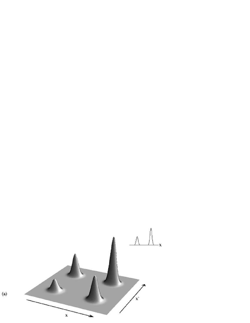
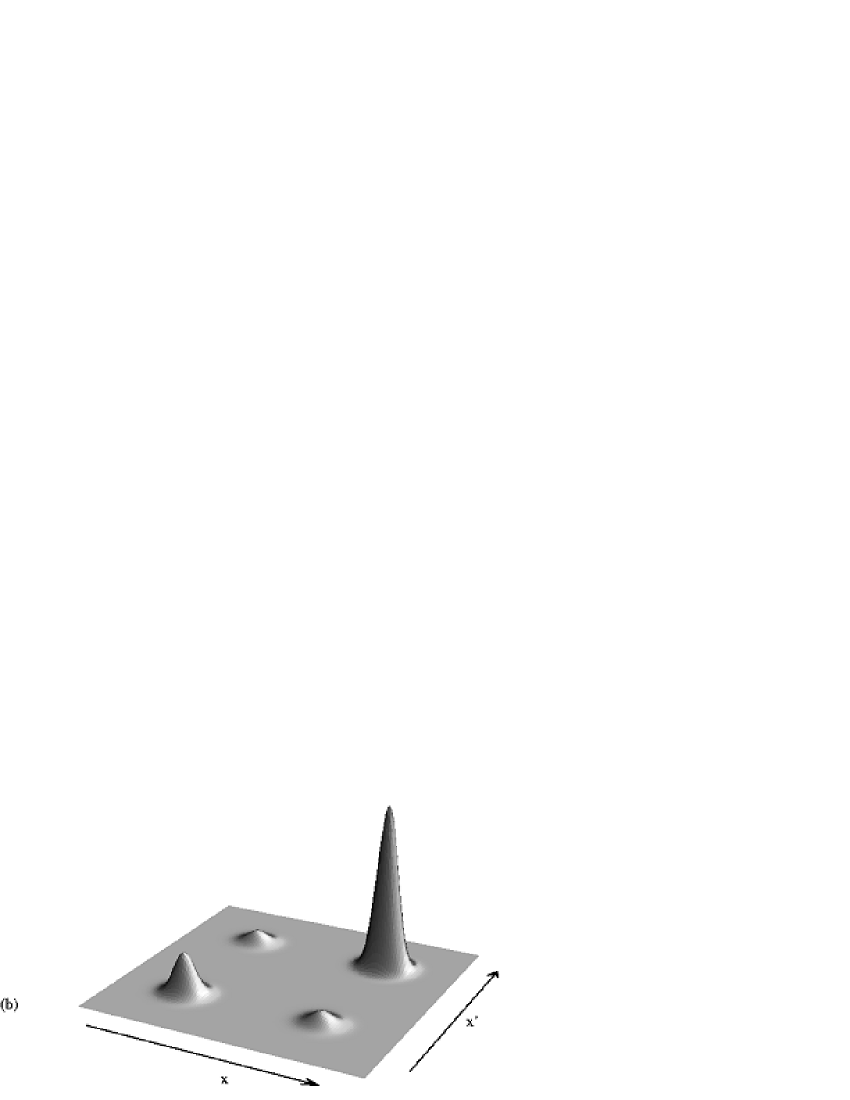
Figure 1: (a) Density matrix of a superposition of two Gaussian wave packets. The wave function is shown in the inset. Coherence between the two parts of the wave function is represented by the two off-diagonal peaks. (b) The density matrix after interference is partially destroyed by decoherence. The position distribution, along the diagonal, is not changed appreciably.

Decoherence according to (13) leads to damping of off-diagonal terms, whereas the peaks near the diagonal are not affected appreciably (this is a property of an ideal measurement). Thus the density matrix develops into a mixture of two packets, as shown in Fig. 1b.

The same effect can be described by using the Wigner function, which is given in terms of the density matrix as

$$W(x,p)=\frac{1}{\pi}\int_{-\infty}^{\infty}\D y\ \E^{2\I py}\rho(x-y,x+y)\ .$$ (15)

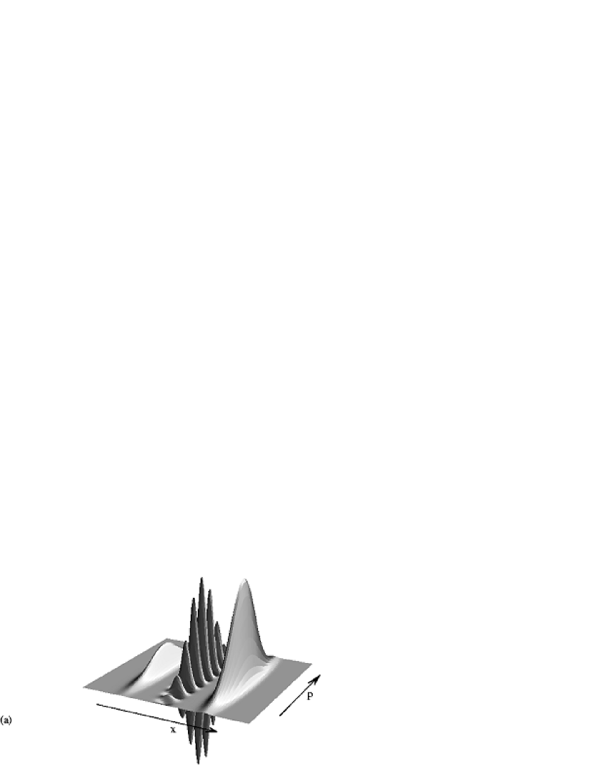
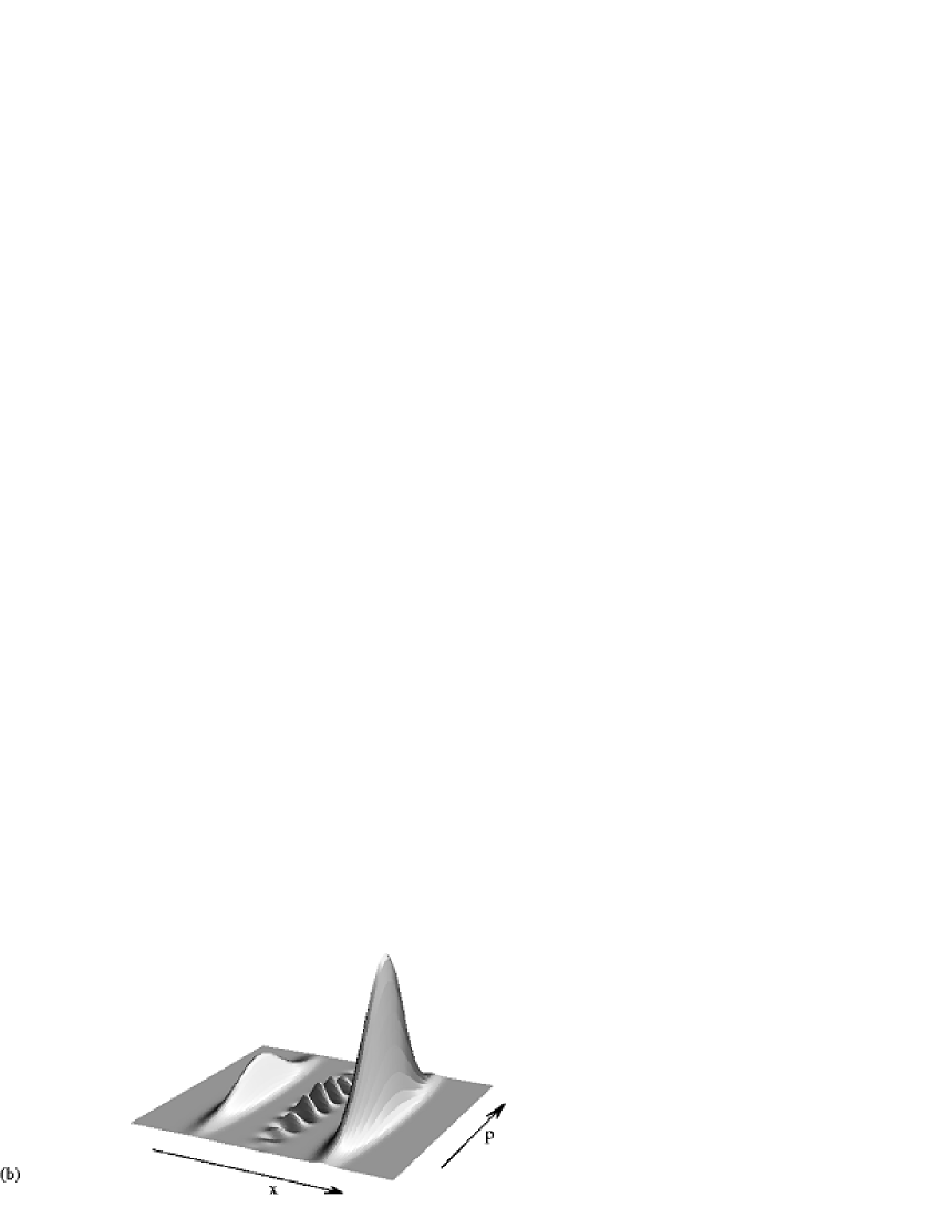
Figure 2: The Wigner function equivalent to the density matrices shown in Fig. 1. (a) represents the superposition of two Gaussian wave packets. Strong oscillations together with negative values indicate coherence between the two wave packets. (b) oscillations are partially damped by decoherence.

A typical feature of the Wigner function are the oscillations occurring for “nonclassical” states, as can be seen in Fig. 2a. These oscillations are damped by decoherence, so that the Wigner function looks more and more like a classical phase space distribution (Fig. 2b). One should keep in mind, however, that the Wigner function is only a useful calculational tool and does not describe a genuine phase space distribution of particles (which do not exist in quantum theory).

The following figures show the analogous situation for an eigenstate of a harmonic oscillator.

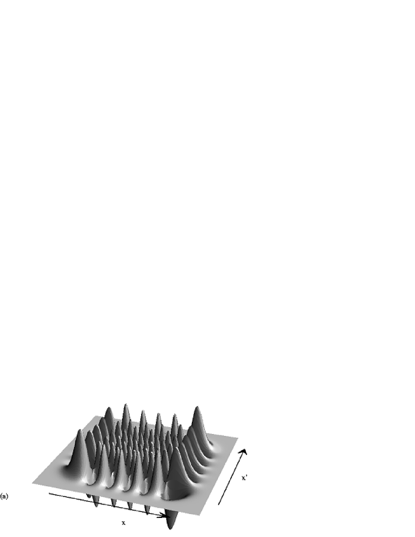
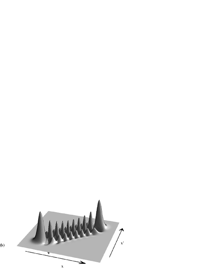
Figure 3: (a)Density matrix of an energy eigenstate of a harmonic oscillator for n=9 in the position representation. (b) Non-diagonal terms are damped by decoherence.

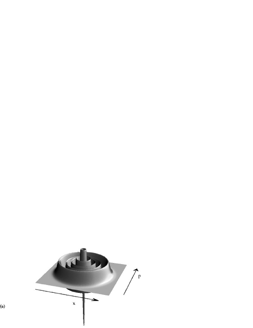
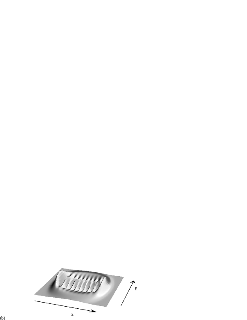
Figure 4: (a)Wigner function for an energy eigenstate of a harmonic oscillator with n=9. The figure shows strong oscillations indicating the non-classical character of this pure state. (b) Decoherence acts like diffusion in this representation. Note that the symmetry between position and momentum is broken by the interaction with the environment.

Combining the decohering effect of scattering processes with the internal dynamics of a “free” particle leads (as in (7)) to a Boltzmann-type master equation which in one dimension is of the form

$$\I\frac{\partial\rho}{\partial t}=[H,\rho]-\I\Lambda[x,[x,\rho]]$$ (16)

and reads explicitly

$$\I\frac{\partial\rho(x,x^{\prime},t)}{\partial t}=\frac{1}{2m}\left(\frac{\partial^{2}}{\partial x^{\prime 2}}-\frac{\partial^{2}}{\partial x^{2}}\right)\rho-\I\Lambda(x-x^{\prime})^{2}\rho\ .$$ (17)

Solutions can easily be found for these equations (see Appendix 2 in Giulini et al. 1996). Let us look at one typical quantum property, the coherence length. According to the Schrödinger equation, a free wave packet would spread, thereby increasing its size and extending its coherence properties over a larger region of space. Decoherence is expected to counteract this behaviour and reduce the coherence length. This can be seen in the solution shown in Fig. 5, where the time dependence of the coherence length (the width of the density matrix in the off-diagonal direction) is plotted for a truly free particle (obeying a Schrödinger equation) and also for increasing strength of decoherence. For large times the spreading of the wave packet no longer occurs and the coherence length always decreases proportional to $1/\sqrt{\Lambda t}$.

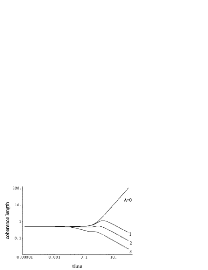
Figure 5: Time dependence of coherence length. It is a measure of the spatial extension over which the object can show interference effects. Except for zero coupling ($\Lambda=0$), the coherence length always decreases for large times.

Is all this just the effect of thermalization? There are several models for the quantum analogue of Brownian motion, some of which are even older than the first decoherence studies. Early treatments did not, however, draw a distinction between decoherence and friction. As an example, consider the equation of motion derived by Caldeira and Leggett (1983),

$$\I\frac{\partial\rho}{\partial t}=[H,\rho]+\frac{\gamma}{2}[x,\{p,\rho\}]-\I m\gamma k_{B}T[x,[x,\rho]]$$ (18)

which reads in one space dimension of a “free” particle

$$\I\frac{\partial\rho(x,x^{\prime},t)}{\partial t} = \left[\frac{1}{2m}\left(\frac{\partial^{2}}{\partial x^{\prime 2}}-\frac{\partial^{2}}{\partial x^{2}}\right)-\I\Lambda(x-x^{\prime})^{2}\right.$$ (19)

$$\left.+\I\gamma(x-x^{\prime})\left(\frac{\partial}{\partial x^{\prime}}-\frac{\partial}{\partial x}\right)\right]\rho(x,x^{\prime},t)\ ,$$

where $\gamma$ is the damping constant and here $\Lambda=m\gamma k_{B}T$. If one compares the effectiveness of the two terms representing decoherence and relaxation, one finds that their ratio is given by

$$\frac{\mbox{decoherence rate}}{\mbox{relaxation rate}}=mk_{B}T(\delta x)^{2}\propto\left(\frac{\delta x}{\lambda_{th}}\right)^{2}\ ,$$ (20)

where $\lambda_{th}$ denotes the thermal de Broglie wavelength. This ratio has for a typical macroscopic situation ($m=1\mbox{g}$, $T=300\mbox{K}$, $\delta x=1\mbox{cm}$) the enormous value of about $10^{40}$! This shows that in these cases decoherence is far more important than dissipation.

Not only the centre-of-mass position of dust particles becomes “classical” via decoherence. The spatial structure of molecules represents another most important example. Consider a simple model of a chiral molecule (Fig. 6).

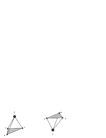
Figure 6: Typical structure of an optically active, chiral molecule. Both versions are mirror-images of each other and are not connected by a proper rotation, if the four elements are different.

Right- and left-handed versions both have a rather well-defined spatial structure, whereas the ground state is - for symmetry reasons - a superposition of both chiral states. These chiral configurations are usually separated by a tunneling barrier (compare Fig. 7) which is so high that under normal circumstances tunneling is very improbable, as was already shown by Hund in 1929. But this alone does not explain why chiral molecules are never found in energy eigenstates!

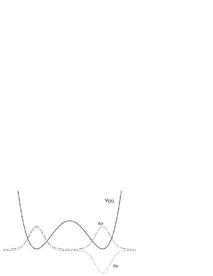
Figure 7: Effective potential for the inversion coordinate in a model for a chiral molecule and the two lowest-lying eigenstates. The ground state is symmetrically distributed over the two wells. Only linear combinations of the two lowest-lying states are localised and correspond to a classical configuration.

In a simplified model with low-lying nearly-degenerate eigenstates $|1\rangle$ and $|2\rangle$, the right- and left-handed configurations may be given by

$$|L\rangle = \frac{1}{\sqrt{2}}(|1\rangle+|2\rangle)$$

$$|R\rangle = \frac{1}{\sqrt{2}}(|1\rangle-|2\rangle)\ .$$ (21)

Because the environment recognises the spatial structure, only chiral states are stable against decoherence,

$$|R,L\rangle|\Phi_{0}\rangle\stackrel{{\scriptstyle t}}{{\longrightarrow}}|R,L\rangle|\Phi_{R,L}\rangle\ .$$ (22)

Additionally, transitions between spatially oriented states are suppressed by the quantum Zeno effect, described below.

3.2 Quantum Zeno Effect

The most dramatic consequence of a strong measurement-like interaction of a system with its environment is the quantum Zeno effect. It has been discovered several times and is also sometimes called “watchdog effect” or “watched pot behaviour”, although most people now use the term Zeno effect. It is surprising only if one sticks to a classical picture where observing a system and just verifying its state should have no influence on it. Such a prejudice is certainly formed by our everyday experience, where observing things in our surroundings does not change their behaviour. As is known since the early times of quantum theory, observation can drastically change the observed system.

The essence of the Zeno effect can easily be shown as follows. Consider the “decay” of a system which is initially prepared in the “undecayed” state $|u\rangle$. The probability to find the system undecayed, i.e., in the same state $|u\rangle$ at time $t$ is for small time intervals given by

$$P(t) = |\langle u|\exp(-\I Ht)|u\rangle|^{2}$$ (23)

$$= 1-(\Delta H)^{2}t^{2}+{\cal O}(t^{4})$$

with

$$(\Delta H)^{2}=\langle u|H^{2}|u\rangle-\langle u|H|u\rangle^{2}\ .$$ (24)

If we consider the case of $N$ measurements in the interval $[0,t]$, the non-decay probability is given by

$$P_{N}(t)\approx\left[1-(\Delta H)^{2}\left(\frac{t}{N}\right)^{2}\right]^{N}>1-(\Delta H)^{2}t^{2}=P(t)\ .$$ (25)

This is always larger than the single-measurement probability given by (23). In the limit of arbitrary dense measurements, the system no longer decays,

$$P_{N}(t)=1-(\Delta H)^{2}\frac{t^{2}}{N}+\ldots\stackrel{{\scriptstyle N\to\infty}}{{\longrightarrow}}1\ .$$ (26)

Hence we find that repeated measurements can completely hinder the natural evolution of a quantum system. Such a result is clearly quite distinct from what is observed for classical systems. Indeed, the paradigmatic example for a classical stochastic process, exponential decay,

$$P(t)=\exp(-\Gamma t)\ ,$$ (27)

is not influenced by repeated observations, since for $N$ measurements we simply have

$$P_{N}(t)=\left(\exp\left(-\Gamma\frac{t}{N}\right)\right)^{N}=\exp(-\Gamma t)\ .$$ (28)

So far we have treated the measurement process in our discussion of the Zeno effect in the usual way by assuming a collapse of the system state onto the subspace corresponding to the measurement result. Such a treatment can be extended by employing a von Neumann model for the measurement process, e.g., by coupling a pointer to a two-state system. A simple toy model is given by the Hamiltonian

$$H = H_{0}+H_{int}$$ (29)

$$= V(|1\rangle\langle 2|+|2\rangle\langle 1|)+E|2\rangle\langle 2|+\gamma\hat{p}(|1\rangle\langle 1|-|2\rangle\langle 2|)\ ,$$

where transitions between states $|1\rangle$ and $|2\rangle$ (induced by the “perturbation” V) are monitored by a pointer (coupling constant $\gamma$). This model already shows all the typical features mentioned above (see Fig. 8).

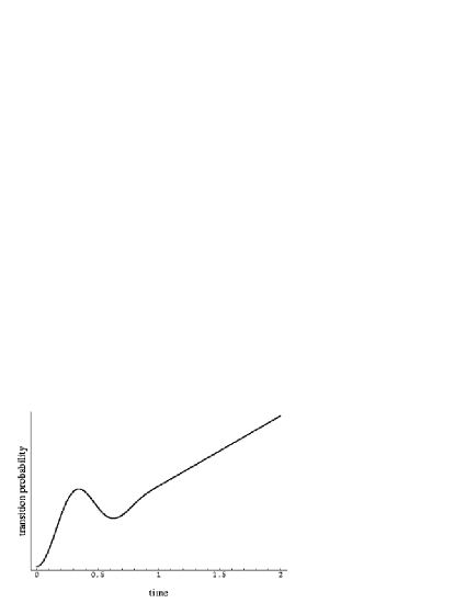
Figure 8: Time dependence of the probability of finding state $|2\rangle$ if the system was prepared in $|1\rangle$ at $t=0$ under continuous coupling to a meter.

The transition probability starts for small times always quadratically, according to the general result (23). For times, where the pointer resolves the two states, a behaviour similar to that found for Markow processes appears: The quadratic time-dependence changes to a linear one.

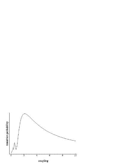
Figure 9: Probability of finding state $|2\rangle$ at a fixed time as a function of the coupling to the meter.

Fig. 9 displays the transition probability as a function of the coupling strength. For strong couling the transitions are suppressed. This clearly shows the dynamical origin of the Zeno effect.

An extension of the above model allows an analysis of the transition from the Zeno effect to master behaviour (described by transition rates as was first studied by Pauli in 1928). It can be shown that for many (micro-) states which are not sufficiently resolved by the environment, Fermi’s Golden Rule can be recovered, with transition rates which are no longer reduced by the Zeno effect. Nevertheless, interference between macrostates is suppressed very rapidly (Joos 1984).

3.3 An example from Quantum Electrodynamics

The occurrence of decoherence is a general phenomenon in quantum theory and is by no means restricted to nonrelativistic quantum mechanics. The following two sections are devoted to decoherence in QED and quantum gravity. It is obvious that the discussion there is technically more involved, and these areas are therefore less studied. However, interesting physical aspects turn out from an understanding of decoherence in this context.

Two situations are important for decoherence in QED, which are, however, two sides of the same coin (Giulini et al. 1996):

• “Measurement” of charges by fields;

• “Measurement” of fields by charges.

In both cases the focus is, of course, on quantum entanglement between states of charged fields with the electromagnetic field, but depending on the given situation, the roles of “relevant” and “irrelevant” parts can interchange.

Considering charges as the relevant part of the total system, it is important to note that every charge is naturally correlated with its Coulomb field. This is a consequence of the Gauß constraint. Superpositions of charges are therefore nonlocal quantum states. This lies at the heart of the charge superselection rule: Locally no such superpositions can be observed, since they are decohered by their entanglement with the Coulomb fields.

A different, but related, question is how far, for example, a wave packet with one electron can be spatially separated and coherently combined again. Experiments show that this is possible over distances in the millimetre range. Coulomb fields act reversibly and cannot prevent the parts of the electronic wave packet from coherently recombining. Genuine, irreversible, decoherence is achieved by emission of real photons. A full QED calculation for this decoherence process is elusive, although estimates exist (Giulini et al. 1996).

Let us now focus on the second part, the decoherence of the electromagnetic field through entanglement with charges. A field theoretic calculation was first done by Kiefer (1992) in the framework of the functional Schrödinger picture for scalar QED. One particular example discussed there is the superposition of a semiclassical state for the electric field pointing upwards with the analogous one pointing downwards,

$$|\Psi\rangle\approx|E\rangle|\chi_{E}\rangle+|-E\rangle|\chi_{-E}\rangle\ ,$$ (30)

where the states $|\chi\rangle$ depend on $E$ and represent states for the charged field. The state $\Psi$ is an approximate solution to the full functional Schrödinger equation. The corresponding reduced density matrix for the electric field shows four “peaks”, in analogy to the case shown in Fig. 1. We take as an example a Gaussian state for the charged fields, representing an adiabatic vacuum state. Integrating out the charged fields from (30), the interference terms (non-diagonal elements) become suppressed, while the probabilities (diagonal elements) are only a slightly changed, corresponding to an almost ideal measurement. In particular, one gets for the non-diagonal elements $\rho_{\pm}=\rho_{\mp}^{*}$:

$$\rho_{\pm}\stackrel{{\scriptstyle t}}{{\longrightarrow}}\rho_{\pm}(D_{V}+D_{PC})\ ,$$ (31)

where $D_{V}$ is the contribution from vacuum polarisation (having a reversible effect like the Coulomb field) and $D_{PC}$ is the contribution from particle creation (giving the typical irreversible behaviour of decoherence). The explicit results are

$$D_{V} = \exp\left(-\frac{Vt}{256\pi^{2}}\frac{(eE)^{3}}{m^{2}+(eEt)^{2}}-\frac{V(eE)^{2}}{256\pi^{2}m}\arctan\frac{eEt}{m}\right)$$ (32)

$$\stackrel{{\scriptstyle t\gg m/eE}}{{\longrightarrow}} \exp\left(-\frac{Ve^{2}E^{2}}{512\pi m}\right)$$

and

$$D_{PC}=\exp\left(-\frac{Vte^{2}E^{2}}{4\pi^{2}}\E^{-\pi m^{2}/eE}\right)\ .$$ (33)

Here, $m$ is the mass of the charged field, and $V$ is the volume; the system has to be enclosed in a finite box to avoid infrared singularities. There is a critical field strength $E_{c}\equiv m^{2}/e$, above which particle creation is important (recall Schwinger’s pair creation formula). For $E<E_{c}$, the usual irreversible decoherence is negligible and only the contribution from vacuum polarisation remains. On the other hand, for $E>E_{c}$, particle creation is dominating, and one has

$$\left|\frac{\ln D_{V}}{\ln D_{PC}}\right|\propto\frac{\pi^{2}}{128mt}\stackrel{{\scriptstyle t}}{{\longrightarrow}}0\ .$$ (34)

Using the influence functional method, the same result was found by Shaisultanov (1995a). He also studied the same situation for fermionic QED and found a somewhat stronger effect for decoherence, see Shaisultanov (1995b). The above result is consistent with the results of Habib et al. (1996) who also found that decoherence due to particle creation is most effective.

3.4 Decoherence in Gravity Theory

In the traditional Copenhagen interpretation of quantum theory, an a priori classical part of the world is assumed to exist from the outset. Such a structure is there thought to be necessary for the “coming into being” of observed measurement results (according to John Wheeler, only an observed phenomenon is a phenomenon). The programme of decoherence, on the other hand, demonstrates that the emergence of classical properties can be understood within quantum theory, without a classical structure given a priori. The following discussion will show that this also holds for the structure that one might expect to be the most classical – spacetime itself.

In quantum theories of the gravitational field, no classical spacetime exists at the most fundamental level. Since it is generally assumed that the gravitational field has to be quantised, the question again arises how the corresponding classical properties arise.

Genuine quantum effects of gravity are expected to occur for scales of the order of the Planck length $\sqrt{G\hbar/c^{3}}$. It is therefore argued that the spacetime structure at larger scales is automatically classical. However, this Planck scale argument is as insufficient as the large mass argument in the evolution of free wave packets. As long as the superposition principle is valid (and even superstring theory leaves this untouched), superpositions of different metrics should occur at any scale.

The central problem can already be demonstrated in a simple Newtonian model. Following Joos (1986), we consider a cube of length $L$ containing a homogeneous gravitational field with a quantum state $\psi$ such that at some initial time $t=0$

$$|\psi\rangle=c_{1}|g\rangle+c_{2}|g^{\prime}\rangle,\;g\neq g^{\prime}\ ,$$ (35)

where $g$ and $g^{\prime}$ correspond to two different field strengths. A particle with mass $m$ in a state $|\chi\rangle$, which moves through this volume, “measures” the value of $g$, since its trajectory depends on the metric:

$$|\psi\rangle|\chi^{(0)}\rangle\to c_{1}|g\rangle|\chi_{g}(t)\rangle+c_{2}|g^{\prime}\rangle|\chi_{g^{\prime}}(t)\rangle\ .$$ (36)

This correlation destroys the coherence between $g$ and $g^{\prime}$, and the reduced density matrix can be estimated to assume the following form after many such interactions are taken into account:

$$\rho(g,g^{\prime},t)=\rho(g,g^{\prime},0)\exp\left(-\Gamma t(g-g^{\prime})^{2}\right),$$ (37)

where

$$\Gamma=nL^{4}\left(\frac{\pi m}{2k_{{B}}T}\right)^{3/2}$$

for a gas with particle density $n$ and temperature $T$. For example, air under ordinary conditions, and $L=1\mbox{ cm}$, $t=1\mbox{ s}$ yields a remaining coherence width of $\Delta g/g\approx 10^{-6}$.

Thus, matter does not only tell space to curve but also to behave classically. This is also true in full quantum gravity. Although such a theory does not yet exist, one can discuss this question within present approaches to quantum gravity. In this respect, canonical quantum gravity fully serves this purpose (Giulini et al. 1996). Two major ingredients are necessary for the emergence of a classical spacetime:

• A type of Born-Oppenheimer approximation for the gravitational field. This gives a semiclassical state for the gravitational part and a Schrödinger equation for the matter part in the spacetime formally defined thereby. Since also superstring theory should lead to this level in some limit, the treatment within canonical gravity is sufficient.

• The quantum entanglement of the gravitational field with irrelevant degrees of freedom (e.g. density perturbations) leads to decoherence for the gravitational field. During this process, states become distinguished that have a well-defined time (which is absent in full quantum gravity). This symmetry breaking stands in full analogy to the symmetry breaking for parity in the case of chiral molecules, see Figs. 6 and 7.

The division between relevant and irrelevant degrees of freedom can be given by the division between semiclassical degrees of freedom (defining the “background”) and others. For example, the relevant degrees of freedom may be the scale factor $a$ of a Friedmann universe containing a global scalar field, $\phi$, like in models for the inflationary universe. The irrelevant degrees of freedom may then be given by small perturbations of these background variables, see Zeh (1986). Explicit calculations then yield a large degree of classicality for $a$ and $\phi$ through decoherence (Kiefer 1987). It is interesting to note that the classicality for $a$ is a necessary prerequisite for the classicality of $\phi$.

Given then the (approximate) classical nature of the spacetime background, decoherence plays a crucial role for the emergence of classical density fluctuations serving as seeds for galaxies and clusters of galaxies (Kiefer, Polarski, and Starobinsky 1998): In inflationary scenarios, all structure emerges from quantum fluctuations of scalar field and metric perturbations. If these modes leave the horizon during inflation, they become highly squeezed and enter as such the horizon in the radiation dominated era. Because of this extreme squeezing, the field amplitude basis becomes a “quantum nondemolition variable”, i.e. a variable that – in the Heisenberg picture – commutes at different times. Moreover, since squeezed states are extremely sensitive to perturbations through interactions with other fields, the field amplitude basis becomes a perfect pointer basis by decoherence. For these reasons, the fluctuations observed in the microwave background radiation are classical stochastic quantities; their quantum origin is exhibited only in the Gaussian nature of the initial conditions.

Because the gravitational field universally interacts with all other degrees of freedom, it is the first quantity (at least its “background part”) to become classical. Arising from the different types of interaction, this gives rise to the following hierarchy of classicality:

Gravitational background variables

$\downarrow$

Other background variables

$\downarrow$

Field modes leaving the horizon

$\downarrow$

Galaxies, clusters of galaxies

$\downarrow$

…

It must be emphasised that decoherence in quantum gravity is not restricted to cosmology. For example, a superposition of black and white hole may be decohered by interaction with Hawking radiation (Demers and Kiefer 1996). However, this only happens if the black holes are in semiclassical states. For virtual black-and-white holes no decoherence, and therefore no irreversible behaviour, occurs.

4 Interpretation

The discussion of the examples in the previous Section clearly demonstrates the ubiquitous nature of decoherence – it is simply not consistent to treat most systems as being isolated. This can only be assumed for microscopic systems such as atoms or small molecules.

In principle, decoherence could have been studied already in the early days of quantum mechanics and, in fact, the contributions of Landau, Mott, and Heisenberg at the end of the twenties can be interpreted as a first step in this direction. Why did one not go further at that time? One major reason was certainly the advent of the “Copenhagen doctrine” that was sufficient to apply the formalism of quantum theory on a pragmatic level. In addition, the imagination of objects being isolable from their environment was so deeply rooted since the time of Galileo, that the quantitative aspect of decoherence was largely underestimated. This quantitative aspect was only born out from detailed calculations, some of which we reviewed above. Moreover, direct experimental verification was only possible quite recently.

What are the achievements of the decoherence mechanism? Decoherence can certainly explain why and how within quantum theory certain objects (including fields) appear classical to “local” observers. It can, of course, not explain why there are such local observers at all. The classical properties are thereby defined by the pointer basis for the object, which is distinguished by the interaction with the environment and which is sufficiently stable in time. It is important to emphasise that classical properties are not an a priori attribute of objects, but only come into being through the interaction with the environment.

Because decoherence acts, for macroscopic systems, on an extremely short time scale, it appears to act discontinuously, although in reality decoherence is a smooth process. This is why “events”, “particles”, or “quantum jumps” are being observed. Only in the special arrangement of experiments, where systems are used that lie at the border between microscopic and macroscopic, can this smooth nature of decoherence be observed.

Since decoherence studies only employ the standard formalism of quantum theory, all components characterising macroscopically different situations are still present in the total quantum state which includes system and environment, although they cannot be observed locally. Whether there is a real dynamical “collapse” of the total state into one definite component or not (which would lead to an Everett interpretation) is at present an undecided question. Since this may not experimentally be decided in the near future, it has been declared a “matter of taste” (Zeh 1997).

Much of the discussion at this conference dealt with the question of how a theory with “definite events” can be obtained. Since quantum theory without any collapse can immediately give the appearance of definite events, it is important to understand that such theories should possess additional features that make them amenable to experimental test. For dynamical collapse models such as the GRW-model or models invoking gravity (see Chap. 8 in Giulini et al. 1996), the collapse may be completely drowned by environmental decoherence, and would thus not be testable, see in particular Bose, Jacobs, and Knight (1997) for a discussion of the experimental situation. As long as no experimental hints about testable additional features are available, such theories may be considered as “excess baggage”, because quantum theory itself can already explain everything that is observed. The price to pay, however, is a somewhat weird concept of reality that includes for the total quantum state all these macroscopically different components.

The most important feature of decoherence besides its ubiquity is its irreversible nature. Due to the interaction with the environment, the quantum mechanical entanglement increases with time. Therefore, the local entropy for subsystems increases, too, since information residing in correlations is locally unobservable. A natural prerequisite for any such irreversible behaviour, most pronounced in the Second Law of thermodynamics, is a special initial condition of very low entropy. Penrose has convincingly demonstrated that this is due to the extremely special nature of the big bang. Can this peculiarity be explained in any satisfactory way? Convincing arguments have been put forward that this can only be achieved within a quantum theory of gravity (Zeh 1992). Since this discussion lies outside the scope of this contribution, it will not be described here.

What is the “Quantum Future” of decoherence? Two important issues play, in our opinion, a crucial role. First, experimental tests should be extended to various situations where a detailed comparison with theoretical calculations can be made. This would considerably improve the confidence in the impact of the decoherence process. It would also be important to study potential situations where collapse models and decoherence would lead to different results. This could lead to the falsification of certain models. An interesting experimental situation is also concerned with the construction of quantum computers where decoherence plays the major negative role. Second, theoretical calculations of concrete decoherence processes should be extended and refined, in particular in field theoretical situations. This could lead to a more profound understanding of the superselection rules frequently used in these circumstances.

Acknowledgements. C.K. thanks the organisers of the Tenth Max Born Symposium, Philippe Blanchard and Arkadiusz Jadczyk, for inviting him to this interesting and stimulating meeting.

References

- [1] Bose, S., Jacobs, K., Knight, P.L. (1997): A scheme to probe the decoherence of a macroscopic object. Report quant-ph/9712017
- [2] Brune, M., Hagley, E., Dreyer, J., Maître, X., Maali, A., Wunderlich, C., Raimond, J.M., Haroche, S. (1996): Observing the Progressive Decoherence of the “Meter” in a Quantum Measurement. Phys. Rev. Lett. 77, 4887–4890
- [3] Caldeira, A.O., Leggett, A.J. (1983): Path integral approach to quantum Brownian motion. Physica 121A, 587–616
- [4] Demers, J.-G., Kiefer, C. (1996): Decoherence of black holes by Hawking radiation. Phys. Rev. D 53, 7050–7061
- [5] Giulini, D., Joos, E., Kiefer, C., Kupsch, J., Stamatescu, I.-O., Zeh, H.D. (1996): Decoherence and the Appearance of a Classical World in Quantum Theory (Springer, Berlin).
- [6] Habib, S., Kluger, Y., Mottola, E., Paz, J.P. (1996): Dissipation and decoherence in mean field theory. Phys. Rev. Lett. 76, 4660–4663
- [7] Heisenberg, W. (1958): Die physikalischen Prinzipien der Quantentheorie. (Bibliographisches Institut, Mannheim)
- [8] Jammer, M. (1974): The Philosophy of Quantum Mechanics (Wiley, New York)
- [9] Joos, E. (1984): Continuous measurement: Watchdog effect versus golden rule. Phys. Rev. D 29, 1626–1633
- [10] Joos, E. (1986): Why do we observe a classical spacetime? Phys. Lett. A 116, 6–8
- [11] Joos, E., Zeh, H.D. (1985): The emergence of classical properties through interaction with the environment. Z. Phys. B 59, 223–243
- [12] Kiefer, C. (1987): Continuous measurement of mini-superspace variables by higher multipoles. Class. Quantum Grav. 4, 1369–1382
- [13] Kiefer, C. (1992): Decoherence in quantum electrodynamics and quantum cosmology. Phys. Rev. D 46, 1658–1670
- [14] Kiefer, C., Polarski, P., Starobinsky, A.A. (1998): Quantum-to-classical transition for fluctuations in the early universe. Submitted to Int. Journ. Mod. Phys. D [Report gr-qc/9802003]
- [15] Kübler, O., Zeh, H.D. (1973): Dynamics of quantum correlations. Ann. Phys. (N.Y.) 76, 405–418
- [16] Landau, L. (1927): Das Dämpfungsproblem in der Wellenmechanik. Z. Phys. 45, 430–441
- [17] Mott, N.F. (1929): The wave mechanics of -ray tracks. Proc. R. Soc. Lond. A 126, 79–84
- [18] Omnès, R. (1997): General theory of the decoherence effect in quantum mechanics. Phys. Rev. A 56, 3383–3394
- [19] Shaisultanov, R.Z. (1995a): Backreaction in scalar QED, Langevin equation and decoherence functional. Report hep-th/9509154
- [20] Shaisultanov, R.Z. (1995b): Backreaction in spinor QED and decoherence functional. Report hep-th/9512144
- [21] Zeh, H.D. (1970): On the interpretation of measurement in quantum theory. Found. Phys. 1, 69–76
- [22] Zeh, H.D. (1986): Emergence of classical time from a universal wave function. Phys. Lett. A 116, 9–12
- [23] Zeh, H.D. (1992): The physical basis of the direction of time (Springer, Berlin)
- [24] Zeh, H.D. (1997): What is achieved by decoherence? In New Developments on Fundamental Problems in Quantum Physics, edited by M. Ferrer and A. van der Merwe (Kluwer Academic, Dordrecht) [Report quant-ph/9610014]
- [25] Zurek, W.H. (1981): Pointer basis of quantum apparatus: Into what mixture does the wave packet collapse? Phys. Rev. D 24, 1516–1525
- [26] Zurek, W.H. (1991): Decoherence and the Transition from Quantum to Classical. Physics Today 44 (Oct.), 36–44; see also the discussion in Physics Today (letters) 46 (April), 13