Quantum state protection in cavities

Abstract

We show how an initially prepared quantum state of a radiation mode in a cavity can be preserved for a long time using a feedback scheme based on the injection of appropriately prepared atoms. We present a feedback scheme both for optical cavities, which can be continuously monitored by a photodetector, and for microwave cavities, which can be monitored only indirectly via the detection of atoms that have interacted with the cavity field. We also discuss the possibility of applying these methods for decoherence control in quantum information processing.

I Introduction

Quantum optics is usually concerned with the generation of nonclassical states of the electromagnetic field and their experimental detection. However with the recent rapid progress in the theory of quantum information processing the protection of quantum states and their quantum dynamics also is becoming a very important issue. In fact what makes quantum information processing much more attractive than its classical counterpart is its capability of using entangled states and of processing generic linear superpositions of input states. The entanglement between a pair of systems is capable of connecting two observers separated by a space-like interval, it can neither be copied nor eavesdropped on without disturbance, nor can it be used by itself to send a classical message [1]. The possibility of using linear superposition states has given rise to quantum computation, which is essentially equivalent to have massive parallel computation [2]. However all these applications crucially rely on the possibility of maintaining quantum coherence, that is, a defined phase relationship between the different components of linear superposition states, over long distances and for long times. This means that one has to minimize as much as possible the effects of the interaction of the quantum system with its environment and, in particular, decoherence, i.e., the rapid destruction of the phase relation between two quantum states of a system caused by the entanglement of these two states with two different states of the environment [3, 4].

Quantum optics is a natural candidate for the experimental implementation of quantum information processing systems, thanks to the recent achievements in the manipulation of single atoms, ions and single cavity modes. In fact two quantum gates have been already demonstrated [5, 6] in quantum optical systems and it would be very important to develop strategies capable of controlling the decoherence in experimental situations such as those described in Refs. [5, 6].

The possibility of an experimental control of decoherence is important also from a more fundamental point of view. In fact decoherence is the practical explanation of why linear superposition of macroscopically distinguishable states, the states involved in the famous Schrödinger cat paradox [7], are never observed and how the classical macroscopic world emerges from the quantum one [3]. In the case of macroscopic systems, the interaction with the environment can never be escaped; since the decoherence rate is proportional to the “macroscopic separation” between the two states [3, 8, 9], a linear superposition of macroscopically distinguishable states is immediately changed into the corresponding statistical mixture, with no quantum coherence left. Nonetheless, a full comprehension of the fuzzy boundary between classical and quantum world is not yet reached [10, 11], and therefore the study of “Schrödinger cat” states in mesoscopic systems where one can hope to observe the decoherence is important. A first achievement has been obtained by Monroe et al. [12], who have prepared a trapped ${\rm{}^{9}Be^{+}}$ ion in a superposition of spatially separated coherent states and detected the quantum coherence between the two localized states. However, in this experiment the decoherence of the superposition state has not been studied. The progressive decoherence of a mesoscopic Schrödinger cat has been observed for the first time in the experiment of Brune et al. [13], where the linear superposition of two coherent states of the electromagnetic field in a cavity with classically distinct phases has been generated and detected.

In this paper we propose a simple physical way to control decoherence and protect a given quantum state against the destructive effects of the interaction with the environment: applying an appropriate feedback. We shall consider a radiation mode in a cavity as the quantum system to protect and we shall show that the “lifetime” of an initial quantum state can be significantly increased and its quantum coherence properties preserved for quite a long time. The feedback scheme considered here has a quantum nature, since it is based on the injection of an appropriately prepared atom in the cavity and some preliminary aspects of the scheme, and its performance, have been described in Refs. [14, 15]. The present paper is a much more detailed description of our approach to quantum state protection and is organized as follows. In Section II, the main idea is presented and a continuous feedback scheme for optical cavities is studied. In Section III, a possible application of this continuous feedback scheme to quantum information processing systems as the quantum phase gate of Ref.  [5] is presented. In the remaining sections, the stroboscopic version of the continuous feedback scheme, more suited for the microwave cavity of the Brune et al. experiment [13], and first introduced in [14], is discussed in detail.

II A feedback loop for optical cavities

Applying a feedback loop to a quantum system means subjecting it to a series of measurements and then using the result of these measurements to modify the dynamics of the system. Very often the system is continuously monitored and the associated feedback scheme provides a continuous control of the quantum dynamics. An example is the measurement of an optical field mode, such as photodetection and homodyne measurements, and for these cases, Wiseman and Milburn have developed a quantum theory of continuous feedback [16]. This theory has been applied in Refs. [17] to show that homodyne-mediated feedback can be used to slow down the decoherence of a Schrödinger cat state in an optical cavity.

Here we propose a different feedback scheme, based on direct photodection rather than homodyne detection. The idea is very simple: whenever the cavity looses a photon, a feedback loop supplies the cavity mode with another photon, through the injection of an appropriately prepared atom. This kind of feedback is naturally suggested by the quantum trajectory picture of a decaying cavity field [18], in which time evolution is driven by the non-unitary evolution operator $\exp\{-\gamma ta^{\dagger}a/2\}$ interrupted at random times by an instantaneous jump describing the loss of a photon. The proposed feedback almost instantaneously “cures” the effect of a quantum jump and is able therefore to minimize the destructive effects of dissipation on the quantum state of the cavity mode.

In more general terms, the application of a feedback loop modifies the master equation of the system and therefore it is equivalent to an effective modification of the dissipative environment of the cavity field. For example, Ref. [19] shows that a squeezed bath [20] can be simulated by the application of a feedback loop based on a quantum non-demolition (QND) measurement of a quadrature of a cavity mode. In other words, feedback is the main tool for realizing, in the optical domain, the so called “quantum reservoir engineering” [21].

The master equation for continuous feedback has been derived by Wiseman and Milburn [16], and, in the case of perfect detection via a single loss source, is given by

$$\dot{\rho}=\gamma\Phi(a\rho a^{\dagger})-\frac{\gamma}{2}a^{\dagger}a\rho-\frac{\gamma}{2}\rho a^{\dagger}a\;,$$ (1)

where $\gamma$ is the cavity decay rate and $\Phi(\rho)$ is a generic superoperator describing the effect of the feedback atom on the cavity state $\rho$. Eq. (1) assumes perfect detection, i.e., all the photons leaving the cavity are absorbed by a unit-efficiency photodetector and trigger the cavity loop. It is practically impossible to realize such an ideal situation and therefore it is more realistic to generalize this feedback master equation to the situation where only a fraction $\eta<1$ of the photons leaking out of the cavity is actually detected and switches on the atomic injector. It is immediate to see that (1) generalizes to

$$\dot{\rho}=\eta\gamma\Phi(a\rho a^{\dagger})+(1-\eta)\gamma a\rho a^{\dagger}-\frac{\gamma}{2}a^{\dagger}a\rho-\frac{\gamma}{2}\rho a^{\dagger}a\;.$$ (2)

Now, we have to determine the action of the feedback atom on the cavity field $\Phi(\rho)$; this atom has to release exactly one photon in the cavity, possibly regardless of the field state in the cavity. In the optical domain this could be realized using adiabatic transfer of Zeeman coherence [22].

A Adiabatic passage in a three level $\Lambda$ atom

A scheme based on the adiabatic passage of an atom with Zeeman substructure through overlapping cavity and laser fields has been proposed [22] for the generation of linear superpositions of Fock states in optical cavities. This technique allows for coherent superpositions of atomic ground state Zeeman sublevels to be “mapped” directly onto coherent superpositions of cavity-mode number states. If one applies this scheme in the simplest case of a three-level $\Lambda$ atom one obtains just the feedback superoperator we are looking for, that is

$$\Phi(\rho)=a^{\dagger}(aa^{\dagger})^{-1/2}\rho(aa^{\dagger})^{-1/2}a\;,$$ (3)

corresponding to the feedback atom releasing exactly one photon into the cavity, regardless the state of the field.

To see this, let us consider a three level $\Lambda$ atom with two ground states $|g_{1}\rangle$ and $|g_{2}\rangle$, coupled to the excited state $|e\rangle$ via, respectively, a classical laser field $\Omega(t)$ of frequency $\omega_{L}$, and a cavity field mode of frequency $\omega$. The corresponding Hamiltonian is

$$H(t)=\hbar\omega a^{\dagger}a+\hbar\omega_{eg}|e\rangle\langle e|-i\hbar g(t)\left(|e\rangle\langle g_{2}|a-|g_{2}\rangle\langle e|a^{\dagger}\right)$$ (4)

$$+i\hbar\Omega(t)\left(|e\rangle\langle g_{1}|e^{-i\omega_{L}t}-|g_{1}\rangle\langle e|e^{i\omega_{L}t}\right)\;.$$ (5)

The time dependence of $\Omega(t)$ and $g(t)$ is provided by the motion of the atom across the laser and cavity profiles. This Hamiltonian couples only states within the three-dimensional manifold spanned by $|g_{1},n\rangle,\,|e,n\rangle,\,|g_{2},n+1\rangle$, where $n$ denotes a Fock state of the cavity mode. Of particular interest within this manifold is the eigenstate corresponding to the adiabatic energy eigenvalue (in the frame rotating at the frequency $\omega$) $E_{n}=n\hbar\omega$,

$$|E_{n}(t)\rangle=\frac{g(t)\sqrt{n+1}|g_{1},n\rangle+\Omega(t)|g_{2},n+1\rangle}{\sqrt{\Omega^{2}(t)+(n+1)g^{2}(t)}}$$ (6)

which does not contain any contribution from the excited state and for this reason is called the “dark state”. This eigenstate exhibits the following asymptotic behavior as a function of time

$$|E_{n}\rangle\rightarrow\left\{\matrix{|g_{1},n\rangle&{\rm for}&\Omega(t)/g(t)\rightarrow 0\cr|g_{2},n+1\rangle&{\rm for}&g(t)/\Omega(t)\rightarrow 0\cr}\right.$$ (7)

Now, according to the adiabatic theorem [23], when the evolution from time $t_{0}$ to time $t_{1}$ is sufficiently slow, a system starting from an eigenstate of $H(t_{0})$ will pass into the corresponding eigenstate of $H(t_{1})$ that derives from it by continuity. This means that if the atom crossing is such that adiabaticity is satisfied, when the atom enters the interaction region in the ground state $|g_{1}\rangle$, the following adiabatic transformation of the atom-cavity system state takes place

$$|g_{1}\rangle\langle g_{1}|\otimes\sum_{n,m}\rho_{n,m}|n\rangle\langle m|$$ (8)

$$\rightarrow|g_{2}\rangle\langle g_{2}|\otimes\sum_{n,m}\rho_{n,m}|n+1\rangle\langle m+1|$$ (9)

$$=|g_{2}\rangle\langle g_{2}|\otimes a^{\dagger}(aa^{\dagger})^{-1/2}\rho(aa^{\dagger})^{-1/2}a\;.$$ (10)

Roughly speaking, this transformation amounts to a single photon transfer from the classical laser field to the quantized cavity mode realized by the crossing atom, provided that a counterintuitive pulse sequence in which the classical laser field $\Omega(t)$ is time-delayed with respect to $g(t)$ is applied. Figure 1 shows a simple diagram of the feedback scheme, together with the appropriate atomic configuration, cavity and laser field profiles needed for the adiabatic transformation considered.

The quantitative conditions under which adiabaticity is satisfied are obtained from the requirement that the transition from the dark state $|E_{n}(t)\rangle$ to the other states be very small. One obtains [22, 24]

$$\Omega_{max},g_{max}\gg T_{cross}^{-1}\;,$$ (11)

where $T_{cross}$ is the cavity crossing time and $\Omega_{max},g_{max}$ are the two peak intensities.

The above arguments completely neglect dissipative effects due to cavity losses and atomic spontaneous emission. For example, cavity dissipation couples a given manifold $|g_{1},n\rangle,\,|e,n\rangle,\,|g_{2},n+1\rangle$ with those with a smaller number of photons. Since ideal adiabatic transfer occurs when the passage involves a single manifold, optimization is obtained when the photon leakage through the cavity is negligible during the atomic crossing, that is

$$T_{cross}^{-1}\gg\bar{n}\gamma\;,$$ (12)

where $\bar{n}$ is mean number of photons in the cavity. On the contrary, the technique of adiabatic passage is robust against the effects of spontaneous emission as, in principle, the excited atomic state $|e\rangle$ is never populated. Of course, in practice some fraction of the population does reach the excited state and hence large values of $g_{max}$ and $\Omega_{max}$ relative to the spontaneous emission rate $\gamma_{e}$ are desirable. To summarize, the quantitative conditions for a practical realization of the adiabatic transformation (8) are

$$\Omega_{max},g_{max}\gg T_{cross}^{-1}\gg\bar{n}\gamma,\gamma_{e}\;,$$ (13)

which, as pointed out in [22], could be realized in optical cavity QED experiments.

We note that when the adiabaticity conditions (13) are satisfied, then also the Markovian assumptions at the basis of the feedback master equation (2) are automatically justified. In fact, the continuous feedback theory of Ref. [16] is a Markovian theory derived assuming that the delay time associated to the feedback loop can be neglected with respect to the typical timescale of the cavity mode dynamics. In the present scheme the feedback delay time is due to the electronic trasmission time of the detection signal and, most importantly, by the interaction time $T_{cross}$ of the atoms with the field, while the typical timescale of the cavity field dynamics is $1/\gamma\bar{n}$. Therefore, the inequality on the right of Eq. (13) is essentially the condition for the validity of the Markovian approximation and this a posteriori justifies our use of the Markovian feedback master equation (2) from the beginning.

B Properties of the adiabatic transfer feedback model

When we insert the explicit expression (3) of the feedback superoperator into Eq. (2), the feedback master equation can be rewritten in the more transparent form

$$\dot{\rho}=\frac{(1-\eta)\gamma}{2}\left(2a\rho a^{\dagger}-a^{\dagger}a\rho-\rho a^{\dagger}a\right)-\frac{\eta\gamma}{2}\left[\sqrt{\hat{n}},\left[\sqrt{\hat{n}},\rho\right]\right]$$ (14)

that is, a standard vacuum bath master equation with effective damping coefficient $(1-\eta)\gamma$ plus an unconventional phase diffusion term, in which the photon number operator is replaced by its square root and which can be called “square root of phase diffusion”.

In the ideal case $\eta=1$, vacuum damping vanishes and only the unconventional phase diffusion survives. As shown in Ref. [25], this is equivalent to say that ideal photodetection feedback is able to transform standard photodetection into a quantum non-demolition (QND) measurement of the photon number. In this ideal case, a generic Fock state $|n\rangle$ is obviously preserved for an infinite time, since each photon lost by the cavity triggers the feedback loop which, in a negligible time, is able to give the photon back through adiabatic transfer. However, the photon injected by feedback has no phase relationship with the photons already present in the cavity and, as shown by (14), this results in phase diffusion. An alternative description of this phenomenon is that the photon injection process is essentially a nonlinear number amplifier which is necessarily accompanied by diffusion in the conjugate variable [26]. This means that feedback does not guarantee perfect state protection for a generic superposition of number states, even in the ideal condition $\eta=1$. In fact in this case, only the diagonal matrix elements in the Fock basis of the initial pure state are perfectly conserved, while the off-diagonal ones always decay to zero, ultimately leading to a phase-invariant state. However this does not mean that the proposed feedback scheme is good for preserving number states only, because the unconventional “square-root of phase diffusion” is much slower than the conventional one (described by a double commutator with the number operator).

In fact the time evolution of a generic density matrix element in the case of feedback with ideal photodetection $\eta=1$ is

$$\rho_{n,m}(t)=\exp\left\{-\frac{\gamma t}{2}\left(\sqrt{n}-\sqrt{m}\right)^{2}\right\}\rho_{n,m}(0)\;,$$ (15)

while the corresponding evolution in the presence of standard phase diffusion is

$$\rho_{n,m}(t)=\exp\left\{-\frac{\gamma t}{2}\left(n-m\right)^{2}\right\}\rho_{n,m}(0)\;.$$ (16)

Since

$$(n-m)^{2}\geq\left(\sqrt{n}-\sqrt{m}\right)^{2}=\frac{(n-m)^{2}}{\left(\sqrt{n}+\sqrt{m}\right)^{2}}\;\;\;\;\;\forall\;n,m\,$$ (17)

each off-diagonal matrix element decays slower in the square root case and this means that the feedback-induced unconventional phase diffusion is slower than the conventional one.

A semiclassical estimation of the diffusion constant can be obtained from the representation of the master equation in terms of the Wigner function. When a generic state is expanded in the Fock basis as

$$\rho=\sum_{n,m}\rho_{n,m}|n\rangle\langle m|\;,$$ (18)

the corresponding Wigner function is given by [27] (in polar coordinates $r,\theta$)

$$W(r,\theta)=\sum_{n}\rho_{n,n}\frac{2}{\pi}(-1)^{n}e^{-2r^{2}}L_{n}(4r^{2})$$ (19)

$$+2{\rm Re}\left\{\sum_{n\neq m}\rho_{n,m}\frac{2}{\pi}(-1)^{n}\sqrt{\frac{n!}{m!}}e^{i\theta(m-n)}\right.$$ (20)

$$\times\left.(2r)^{m-n}e^{-2r^{2}}L^{m-n}_{n}(4r^{2})\right\}\;,$$ (21)

where $L_{n}^{m-n}$ are the generalized Laguerre polynomials and using this expression it is easy to see that

$$-\left[n,\left[n,\rho\right]\right]\leftrightarrow\frac{\partial^{2}}{\partial\theta^{2}}W(r,\theta)\;.$$ (22)

In the case of the square root of phase diffusion, one has instead

$$-\left[\sqrt{n},\left[\sqrt{n},\rho\right]\right]\leftrightarrow 2{\rm Re}\left\{\sum_{n\neq m}\rho_{n,m}\frac{2}{\pi}(-1)^{n}\sqrt{\frac{n!}{m!}}\right.$$ (23)

$$\times\left.\left(\sqrt{n}-\sqrt{m}\right)^{2}e^{i\theta(m-n)}(2r)^{m-n}e^{-2r^{2}}L^{m-n}_{n}(4r^{2})\right\}\;;$$ (24)

using (17) and considering the semiclassical limit $n,m\gg 1$, $n\sim m\sim\bar{n}\gg 1$, where $\bar{n}$ is the mean photon number, (23) can be simplified to

$$-\left[\sqrt{n},\left[\sqrt{n},\rho\right]\right]\leftrightarrow\frac{1}{4\bar{n}}\frac{\partial^{2}}{\partial\theta^{2}}W(r,\theta)\;,$$ (25)

showing that (at least at large photon number) in the case of the feedback-induced unconventional phase diffusion, the diffusion constant is scaled by a factor $4\bar{n}\gg 1$.

A complementary description of the feedback-induced phase diffusion can be given by the time evolution of the mean coherent amplitude $\langle a(t)\rangle$. In fact, phase diffusion causes a decay of this amplitude as the phase spreads around $2\pi$, even if the photon number is conserved. In the presence of ordinary phase diffusion the amplitude decays at the rate $\gamma/2$; in fact

$$\langle a(t)\rangle={\rm Tr}\left\{a\rho(t)\right\}=\sum_{n=0}^{\infty}\sqrt{n+1}\rho_{n+1,n}(t)\;,$$ (26)

and using Eq. (16) one gets

$$\langle a(t)\rangle=e^{-\gamma t/2}\langle a(0)\rangle\;.$$

In the case of the square root of phase diffusion, Eqs. (15) and (26) instead yield

$$\langle a(t)\rangle={\rm Tr}\left\{a(t)\rho(0)\right\}\;,$$ (27)

where the Heisenberg-like time evolved amplitude operator $a(t)$ is given by

$$a(t)=\exp\left\{-\frac{\gamma t}{2}\left(\sqrt{aa^{\dagger}}-\sqrt{a^{\dagger}a}\right)^{2}\right\}a\;.$$ (28)

In the semiclassical limit it is reasonable to assume a complete factorization of averages (27), so to get

$$\langle a(t)\rangle=\exp\left\{-\frac{\gamma t}{2}\left(\sqrt{\bar{n}+1}-\sqrt{\bar{n}}\right)^{2}\right\}\langle a(0)\rangle\;,$$ (29)

which, in the limit of large mean photon number $\bar{n}$, yields a result analogous to that of Eq. (25)

$$\langle a(t)\rangle=\exp\left\{-\frac{\gamma t}{8\bar{n}}\right\}\langle a(0)\rangle\;.$$ (30)

This slowing down of phase diffusion (similar to that taking place in a laser well above threshold) means that, when the feedback efficiency $\eta$ is not too low, the “lifetime” of generic pure quantum states of the cavity field can be significantly increased with respect to the standard case with no feedback (see Eq. 14).

C Description of the dynamics in the presence of feedback

For a quantitative characterization of how the feedback scheme is able to protect an initial pure state we study the fidelity $F(t)$

$$F(t)={\rm Tr}\left\{\rho(0)\rho(t)\right\}$$ (31)

i.e., the overlap between the final and the initial state $\rho(0)$ after a time $t$. In general $0\leq F(t)\leq 1$. For an initially pure state $|\psi(0)\rangle$, $F(t)$ is in fact the probability to find the system in the intial state at a later time. A decay to an asymptotic limit is given by the overlap $\langle\psi(0)|\rho(\infty)|\psi(0)\rangle$.

A clear demonstration of the protection capabilities of the proposed feedback scheme is given when considering the preservation of initial Schrödinger cat state, i.e., the typical example of nonclassical state whose oscillating and non-positive definite Wigner function is a clear signature of quantum coherence [3]. In fact, if the initial state is an even $(+)$ or odd $(-)$ Schrödinger cat state

$$|\alpha_{\pm}\rangle=N_{\pm}\left(|\alpha\rangle\pm|-\alpha\rangle\right)$$ (32)

where

$$N_{\pm}^{-2}=2\left(1\pm e^{-2|\alpha|^{2}}\right)\;,$$ (33)

the corresponding fidelity $F(t)$ in absence of feedback ($\eta=0$ in (14)) is given by

$$F_{\pm}(t)=\frac{1+e^{-2|\alpha|^{2}(1-e^{-\gamma t})}}{2}e^{-|\alpha|^{2}(1-e^{-\gamma t/2})^{2}}$$ (34)

$$\times\left(\frac{1\pm e^{-2|\alpha|^{2}e^{-\gamma t/2}}}{1\pm e^{-2|\alpha|^{2}}}\right)^{2}\;.$$ (35)

The corresponding function $F(t)$ in the presence of feedback can be easily obtained from the numerical solution of the master equation (14) and using the general expression

$$F(t)=\sum_{n,m}\rho_{n,m}^{*}(0)\rho_{n,m}(t)\;.$$ (36)

The numerical results (Fig. 2) show that $F(t)$ in the presence of feedback is, at any time, significantly larger than the corresponding function in absence of feedback, even when the photodetection efficiency $\eta$ is far from the ideal value $\eta=1$. Figure 2 refers to an initial odd cat state with $\alpha=\sqrt{5}$; the full line refers to the feedback model in the ideal case $\eta=1$; the dotted line to the feedback case with $\eta=0.75$, small dashes refer to the case $\eta=0.5$; big dashes refer to $\eta=0.25$ and the dot-dashed line to the evolution in absence of feedback ($\eta=0$). As expected, the preservation properties of the proposed scheme worsen as the photedetection efficiency $\eta$ is decreased. Nonetheless, Figure 2 clearly shows how this photodetection-mediated feedback increases the “lifetime” of a generic pure state in the cavity, in the sense that the probability of finding the initial state at any time $t$ is larger than the corresponding probability in absence of feedback.

A qualitative confirmation of how well an initial odd cat state with $\alpha=\sqrt{5}$ is protected by feedback is given by Figure 3: (a) shows the Wigner function of the initial cat state, (b) the Wigner function of the same cat state evolved for a time $t=0.2/\gamma$ in the presence of feedback ($\eta=1$) and (c) the Wigner function of the same state again after a time $t=0.2/\gamma$, but evolved in absence of feedback. This elapsed time is twice the decoherence time of the Schrödinger cat state, $t_{dec}=(2\gamma|\alpha|^{2})^{-1}$ [8, 9], i.e., the lifetime of the interference terms in the cat state density matrix in the presence of the usual vacuum damping. As it is shown by (c), this means that after this short time the cat state has already lost the oscillating part of the Wigner function associated to quantum interference and has become a statistical mixture of two coherent states. This is no longer true in the presence of our feedback scheme: (b) shows that, after $t\sim 2t_{dec}$, the state is almost indistinguishable from the initial one and that the quantum wiggles of the Wigner function are still well visible. The capability of the feedback scheme of preserving the quantum coherence of the initial cat state for quite a long time is shown also by Fig. 4, in which the Wigner function both in the presence ($\eta=1$) (a) and in absence of feedback (b) of the initial odd cat state of Fig. 3 evolved after one relaxation time $t=\gamma^{-1}$ is shown. In the presence of feedback the oscillating part between the two peaks is still visible, even if the state begins to be distorted with respect to the initial one because of the action of the unconventional phase diffusion which makes it more “rounded”. We obtain, so to speak, a “mangy” cat.

Another clear example of how the quantum coherence associated to nonclassical superposition states of the radiation field inside the cavity is well preserved by the feedback scheme based on the adiabatic passage, is given by the study of the evolution of linear superpositions of two Fock number states

$$|\psi(0)\rangle=\alpha|n\rangle+\beta|m\rangle\;.$$ (37)

These states have not been experimentally generated in optical cavities yet, but there are now a number of proposals for their generation [28, 29]. In this case $F(t)$ can be easily evaluated analytically ($m>n$)

$$F(t)=|\alpha|^{4}e^{-n(1-\eta)\gamma t}+|\beta|^{4}e^{-m(1-\eta)\gamma t}$$ (38)

$$+2|\alpha|^{2}|\beta|^{2}e^{-\gamma t\left[(m+n)/2-\eta\sqrt{nm}\right]}$$ (39)

$$+|\alpha|^{2}|\beta|^{2}e^{-n(1-\eta)\gamma t}\left(1-e^{-(1-\eta)\gamma t}\right)^{m-n}\frac{m!n!}{(m-n)!}$$ (40)

and when this expression is plotted for different values of $\eta$ and compared with that in absence of feedback ($\eta=0$), we see, as in Figure 2, a significant increase of the “lifetime” of the state (37). This comparison is shown in Figure 5, which refers to the initial state $(|2\rangle+\sqrt{2}|4\rangle)/\sqrt{3}$ and where the notation is as in Fig. 2: the full line refers to the feedback model in the ideal case $\eta=1$; the dotted line to the feedback case with $\eta=0.75$, small dashes refer to the case $\eta=0.5$; big dashes refer to $\eta=0.25$ and the dot-dashed line to the evolution in absence of feedback ($\eta=0$).

III Optical feedback scheme for the protection of qubits

Photon states are known to retain their phase coherence over considerable distances and for long times and for this reason high-Q optical cavities have been proposed as a promising example for the realization of simple quantum circuits for quantum information processing. To act as an information carrying quantum state, the electromagnetic fields must consist of a superposition of few distinguishable states. The most straightforward choice is to consider the superposition of the vacuum and the one photon state $\alpha|0\rangle+\beta|1\rangle$. However it is easy to understand that this is not convenient because any interaction coupling $|0\rangle$ and $|1\rangle$ also couples $|1\rangle$ with states with more photons and this leads to information losses. Moreover the vacuum state is not easy to observe because it cannot be distinguished from a failed detection of the one photon state. A more convenient and natural choice is polarization coding, i.e., using two degenerate polarized modes and qubits of the following form

$$|\psi\rangle=\left(\alpha a_{+}^{\dagger}+\beta a_{-}^{\dagger}\right)|0\rangle=\alpha|0,1\rangle+\beta|1,0\rangle\;,$$ (41)

in which one photon is shared by the two modes [30]. In fact this is a “natural” two-state system, in which the two basis states can be easily distinguished with polarization measurements; moreover they can be easily transformed into each other using polarizers. Polarization coding has been already employed in one of the few experimental realization of a quantum gate, the quantum phase gate realized at Caltech [5]. This experiment has demonstrated conditional quantum dynamics between two frequency-distinct fields in a high-finesse optical cavity. The implementation of this gate employs two single-photon pulses with frequency separation large compared to the individual bandwidth, and whose internal state is specified by the circular polarization basis as in (41). The conditional dynamics between the two fields is obtained through an effective strong Kerr-type nonlinearity provided by a beam of cesium atoms.

In the preceding section we have shown that the proposed feedback scheme is able to increase the “lifetime” of linear superpositions of Fock states. Therefore it is quite natural to look if our scheme can be used to protect qubits like those of the Caltech experiment, against the destructive effects of cavity damping. To be more specific, here we shall not be concerned with the protection of the quantum gate dynamics, but we shall focus on a simpler but still important problem: protecting an unknown input state for the longest possible time against decoherence. For this reason we shall not consider the two interacting fields, but a single frequency mode with a generic polarization, i.e., a single qubit. We shall consider a class of initial states more general than those of Eq. (41), i.e.,

$$|\psi\rangle=\alpha|n,m\rangle+\beta|m,n\rangle\;,$$ (42)

where $m+n$ photons are shared by the two polarized modes.

If we want to apply the adiabatic transfer feedback scheme described above for protecting qubits as those of Eq. (42), one has to consider a feedback loop as that of Fig. 1 for each polarized mode. This can be done using polarization-sensitive detectors which electronically control the polarization of the classical laser field and the initial state of the injected atoms. In fact one has to release in the cavity a left or right circularly polarized photon depending on which detector has fired and this can be easily achieved when the $|g_{1}\rangle\rightarrow|e\rangle$ and $|g_{2}\rangle\rightarrow|e\rangle$ transitions are characterized by opposite angular momentum difference $\Delta m_{J}=\pm 1$. In this case a left polarized photon, for example, is given back to the cavity with the adiabatic transition $|g_{1}\rangle\rightarrow|g_{2}\rangle$ of Fig. 1, while the right polarized one is released into the cavity through the reversed adiabatic transition $|g_{2}\rangle\rightarrow|g_{1}\rangle$ and the two possibilities are controlled by the polarization sensitive detectors.

Since the input state we seek to protect is unknown, the protection capabilities of the feedback scheme are better characterized by the minimum fidelity, i.e., the fidelity of Eq. (31) minimized over all possible initial states. This minimum fidelity can be easily evaluated by solving the master equation (14) for each polarized mode and one gets the following expression

$$F_{min}(t)=\frac{1}{2}\left(e^{-(1-\eta)\gamma t(n+m)}+e^{-\gamma t(n+m-2\eta\sqrt{nm})}\right)\;.$$ (43)

In the absence of feedback ($\eta=0$), this expression becomes $F_{min}(t)=\exp\{-\gamma t(n+m)\}$ showing that in this case, the states most robust against cavity damping are those with the smallest number of photons, $m+n=1$, i.e., the states of the form of Eq. (41). Moreover, in a typical quantum information processing situation, one has to consider small qubit “storage” times $t$ with respect to $\gamma^{-1}$ so to have reasonably small error probabilities in quantum information storage. Therefore the protection capability of an optical cavity with no feedback applied is described by

$$F_{min}(t)=1-\gamma t\;.$$ (44)

If we now consider the situation in the presence of feedback (Eq. (43)), the best protected states for a given nonzero efficiency $\eta$, may be different from the states with only one photon, $\alpha|0,1\rangle+\beta|1,0\rangle$, and they depend upon the explicit value of the feedback efficiency $\eta$. For the determination of the optimal qubit of the form of (42) (i.e., the optimal values for $m$ and $n$), one has to minimize the deviation from the perfect protection condition $F(t)=1$. For $\gamma t\ll 1$ one gets

$$\min_{m\neq n}\left[(2-\eta)(n+m)-2\eta\sqrt{nm}\right]$$ (45)

$$=\min_{m\neq n}\left[(\sqrt{m}-\sqrt{n})^{2}+(1-\eta)(\sqrt{m}+\sqrt{n})^{2}\right]$$ (46)

$$=\min_{n\geq 0,\,p\geq 1}\left[\frac{p^{2}}{(\sqrt{n+p}+\sqrt{n})^{2}}+(1-\eta)(\sqrt{n+p}+\sqrt{n})^{2}\right]\;,$$ (47)

where $p=m-n$. From these expression it can be easily seen that one has to choose $p=1$, and therefore the optimal qubits are those of the form

$$|\psi\rangle=\alpha|n_{opt},n_{opt}+1\rangle+\beta|n_{opt}+1,n_{opt}\rangle\;,$$ (48)

where $n_{opt}$ is determined by the minimization condition

$$\min_{n\geq 0}\left[\frac{1}{(\sqrt{n+1}+\sqrt{n})^{2}}+(1-\eta)(\sqrt{n+1}+\sqrt{n})^{2}\right]\;.$$ (49)

As long as

$$\eta\leq 2/(1+\sqrt{2})\simeq 0.83\;,$$ (50)

one has $n_{opt}=0$ and therefore the situation is similar to that of the no-feedback case: the states of the form (41) are the best protected states and the corresponding minimum fidelity is given by

$$F_{min}(t)=\frac{1}{2}\left(e^{-(1-\eta)\gamma t}+e^{-\gamma t}\right)\simeq 1-\gamma t\left(1-\frac{\eta}{2}\right)\;.$$ (51)

In this case, feedback leads to a very poor qubit protection with respect to the no-feedback case and therefore our scheme proves to be practically useless for the protection of single photon qubits of (41) employed in the Caltech experiment of Ref. [5].

However, when the feedback efficiency $\eta$ becomes larger than 0.83, the situation can improve considerably. In fact $n_{opt}$ becomes nonzero and can become very large in the limit $\eta\rightarrow 1$, and in this case the minimum fidelity decays very slowly. To be more specific, $n_{opt}$ is approximately given by the condition

$$\left(\sqrt{n_{opt}+1}+\sqrt{n_{opt}}\right)^{2}=\left(1-\eta\right)^{-1/2}$$ (52)

and the corresponding small time behavior of $F_{min}(t)$ is given by

$$F_{min}(t)\simeq 1-\frac{\gamma t}{\left(\sqrt{n_{opt}+1}+\sqrt{n_{opt}}\right)^{2}}\simeq 1-\gamma t\sqrt{1-\eta}\;.$$ (53)

This means that in the limit of a feedback efficiency very close to one, it becomes convenient to work with a large number of photons per mode, since in this limit the probability of errors in the storage of quantum information can be made very small. This can be easily understood from Eq. (14), because in this limit the square-root of phase diffusion term prevails in the master equation and its quantum state protection capabilities improve for increasing photon number (see Eq. (30)). In the ideal case $\eta=1$, $n_{opt}$ becomes infinite and therefore the minimum fidelity can remain arbitrarily close to one. It is convenient to work with the largest possible number of photons, that is,

$$|\psi\rangle=\alpha|n,n+1\rangle+\beta|n+1,n\rangle\;\;\;\;\;n\gg 1$$ (54)

and the corresponding minimum fidelity is

$$F_{min}(t)\simeq\frac{1}{2}\left(1+e^{-\gamma t/4n}\right)\simeq 1-\frac{\gamma t}{8n}\;.$$

The feedback method proposed here to deal with decoherence in quantum information processing is different from most of the proposals made in this research field, which are based on the so called quantum error correction codes [31], which are a way to use software to preserve linear superposition states. In our case, feedback allows a physical control of decoherence, through a continuous monitoring and eventual correction of the dynamics and in this sense our approach is similar in spirit to the approach of Ref. [32, 33]. The present feedback scheme is not very useful in the case of one-photon qubits (41) of the quantum phase gate experiment of Ref. [5]; however it predicts a very good decoherence control in the case of high feedback efficiency $\eta>0.83$ and for larger photon numbers (see Eq. (48)). It is very difficult to achieve these experimental conditions with the present technology, but our scheme could become very promising in the future.

IV A feedback scheme for microwave cavities

In the case of measurements of an optical field mode, such as photodetection and homodyne measurements, the system is continuously measured and in these cases applying a feedback loop can be quite effective in controlling the decoherence of an optical Schrödinger cat. It is therefore quite natural to see if a similar control of decoherence can be achieved in the only (up to now) experimental generation and detection of Schrödinger cat states of a radiation mode, the experiment of Brune et al [13]. However, in this experiment, it is not possible to monitor continuously the state of the radiation in the cavity, since the involved field is in the microwave range and there are not good enough detectors in this wavelength region. The detection of the cat state is obtained through measurements performed on a second probe atom crossing the cavity after a delay time $T$ and that provides a sort of impulsive measurements of the cavity field state.

This suggests that in this microwave case, continuous measurement can be replaced at best by a series of repeated measurements, performed by off-resonance atoms crossing the high-Q microwave cavity one by one with a time interval $T$. As a consequence, one could try to apply a sort of “discrete” feedback scheme modifying in a “stroboscopic” way the cavity field dynamics according to the result of the atomic detection.

A A simplified description of the experiment of Brune et al.

In Ref. [13], a Schrödinger cat state for the microwave field in a superconducting cavity $C$ has been generated using circular Rydberg atoms crossing the cavity in which a coherent state has been previously injected. All the atoms have an appropriately selected velocity and the relevant levels are two adjacent circular Rydberg states with principal quantum numbers $n=50$ and $n=51$, which we denote as $|g\rangle$ and $|e\rangle$ respectively. These two states have a very long lifetime ($30$ ms) and a very strong coupling to the radiation and the atoms are initially prepared in the state $|e\rangle$. The high-Q superconducting cavity is sandwiched between two low-Q cavities $R_{1}$ and $R_{2}$, in which classical microwave fields can be applied and which are resonant with the transition between the state $|e\rangle$ and the nearby lower circular state $|g\rangle$. The intensity of the field in the first cavity $R_{1}$ is then chosen so that, for the selected atom velocity, a $\pi/2$ pulse is applied to the atom as it crosses $R_{1}$. As a consequence, the atomic state before entering the cavity $C$ is

$$|\psi_{atom}\rangle=\frac{1}{\sqrt{2}}\left(|e\rangle+|g\rangle\right)\;.$$ (55)

The high-Q cavity $C$ is slightly off-resonance with respect to the $e\,\rightarrow\,g$ transition, with detuning

$$\delta=\omega-\omega_{eg}\;,$$ (56)

where $\omega$ is the cavity mode frequency and $\omega_{eg}=(E_{e}-E_{g})/\hbar$. The Hamiltonian of the atom-microwave cavity mode system is the usual Jaynes-Cummings Hamiltonian, given by

$$H_{JC}=E_{e}|e\rangle\langle e|+E_{g}|g\rangle\langle g|+\hbar\omega a^{\dagger}a$$ (57)

$$+\hbar\Omega\left(|e\rangle\langle g|a+|g\rangle\langle e|a^{\dagger}\right)\;,$$ (58)

where $\Omega$ is the vacuum Rabi coupling between the atomic dipole on the $e\,\rightarrow\,g$ transition and the cavity mode. In the off-resonant case and perturbative limit $\Omega\ll\delta$, the atom and the field essentially do not exchange energy but only undergo dispersive frequency shifts depending on the atomic level [34, 35], and the Hamiltonian (58) becomes equivalent to

$$H_{disp}=E_{e}|e\rangle\langle e|+E_{g}|g\rangle\langle g|+\hbar\omega a^{\dagger}a$$ (59)

$$+\hbar\frac{\Omega^{2}}{\delta}\left(|g\rangle\langle g|a^{\dagger}a-|e\rangle\langle e|aa^{\dagger}\right)$$ (60)

$$=\left(E_{e}-\hbar\frac{\Omega^{2}}{\delta}\right)|e\rangle\langle e|+E_{g}|g\rangle\langle g|+\hbar\left(\omega+\frac{\Omega^{2}}{\delta}\right)a^{\dagger}a$$ (61)

$$-2\hbar\frac{\Omega^{2}}{\delta}|e\rangle\langle e|a^{\dagger}a\;.$$ (62)

This means that in this dispersive limit, besides a negligible shift of the cavity frequency and of the $e$ level energy, the atom-field interaction induces a phase shift $\phi=2\Omega^{2}t_{int}/\delta$ when the atom is in the state $e$, while there is no shift when the atom is in the state $g$ ($t_{int}$ is the interaction time). Therefore, using (55), the state of the atom-field system when the atom has just exited the cavity $C$ is the entangled state

$$|\psi_{atom+field}\rangle=\frac{1}{\sqrt{2}}\left(|e,\alpha e^{i\phi}\rangle+|g,\alpha\rangle\right)\;,$$ (63)

where $\alpha$ denotes the coherent state initially present within the cavity. In the experiment of Ref. [13], different values of the phase shift $\phi$ have been considered; however we shall restrict from now on to the case $\phi=\pi$, which corresponds to the generation of a linear superposition of two coherent states with opposite phases.

In the state (63), each atomic state is correlated to a different field phase; for the generation of a cat state, however, one has to correlate each atomic state to a superposition of coherent states with different phases, and this is achieved by submitting the atom to a second $\pi/2$ pulse in the second microwave cavity $R_{2}$. The $\pi/2$ pulse yields the following transformation

$$|e\rangle \rightarrow \frac{1}{\sqrt{2}}\left(|e\rangle+|g\rangle\right)$$ (64)

$$|g\rangle \rightarrow \frac{1}{\sqrt{2}}\left(-|e\rangle+|g\rangle\right)\;,$$ (65)

so that the state (63) becomes

$$|\psi^{\prime}_{atom+field}\rangle=\frac{1}{\sqrt{2}}\left(N_{-}^{-1}|e\rangle|\alpha_{-}\rangle+N_{+}^{-1}|g\rangle|\alpha_{+}\rangle\right)\;.$$ (66)

where $|\alpha_{\pm}\rangle$ are the even $(+)$ or odd $(-)$ Schrödinger cat states defined in (32) and $N_{\pm}$ are defined in Eq. (33). Eq. (66) shows that an even or an odd coherent state is conditionally generated in the cavity according to whether or not the atom is detected in the level $|g\rangle$ or $|e\rangle$, respectively.

After generation, the Schrödinger cat state undergoes a vary fast decoherence process [8, 9], that is, a fast decay of interference terms, caused by the inevitable presence of dissipation in the superconducting cavity. In fact the dissipative time evolution of the generated cat state is described by the following density matrix

$$\rho(t)=\frac{1}{N_{\pm}^{2}}\left[|\alpha e^{-\gamma t/2}\rangle\langle\alpha e^{-\gamma t/2}|+|-\alpha e^{-\gamma t/2}\rangle\langle-\alpha e^{-\gamma t/2}|\right.$$ (67)

$$\left.\pm e^{-2|\alpha|^{2}(1-e^{-\gamma t})}\left(|-\alpha e^{-\gamma t/2}\rangle\langle\alpha e^{-\gamma t/2}|\right.\right.$$ (68)

$$\left.\left.+|\alpha e^{-\gamma t/2}\rangle\langle-\alpha e^{-\gamma t/2}|\right)\right]\;,$$ (69)

where $\gamma$ is the cavity decay rate and where the plus (minus) sign correspond to the even (odd) coherent state. Decoherence is governed by the factor $\exp\left[-2|\alpha|^{2}(1-e^{-\gamma t})\right]$, which for $\gamma t\ll 1$ becomes $\exp\left[-2|\alpha|^{2}\gamma t\right]$, implying therefore that the interference terms decay to zero with a lifetime $t_{dec}=(2\gamma|\alpha|^{2})^{-1}$.

The relevance of the experiment of Brune et al. [13] lies in the fact that this progressive decoherence of the cat state has been observed for the first time and the theoretical prediction checked with no fitting parameters. This monitoring of decoherence has been obtained by sending a second atom through the same arrangements of cavities. The atom has exactly the same velocity of the first atom generating the cat and is sent through the cavities after a time delay $T$, which is much larger than the time of flight of the atom through the whole system (which is of the order of $10^{-5}s$ in the experiment). The state of the system composed by the second atom and the microwave field undergoes the same transformation described above for the first Rydberg atom, i.e.,

$$\rho_{atom+field}$$ (70)

$$=U_{\frac{\pi}{2}}e^{i\pi a^{\dagger}a|e\rangle\langle e|}U_{\frac{\pi}{2}}(\rho(T)\otimes|e\rangle\langle e|)U_{\frac{\pi}{2}}^{\dagger}e^{-i\pi a^{\dagger}a|e\rangle\langle e|}U_{\frac{\pi}{2}}^{\dagger}\;,$$ (71)

where $U_{\frac{\pi}{2}}$ describes the $\pi/2$ pulse and $\rho(T)$ is the cavity field at a time $T$ after the passage of the first atom and it is given by Eq. (69).

Using (65) one finally gets the state of the probe atom+field system just before the field ionization detectors for the measurement of the $e$ or $g$ atomic state, that is,

$$\rho_{atom+field}=|e\rangle\langle e|\otimes\rho_{e}+|g\rangle\langle g|\otimes\rho_{g}$$ (72)

$$+|e\rangle\langle g|\otimes\rho_{+}+|g\rangle\langle e|\otimes\rho_{-}\;,$$ (73)

where

$$\rho_{\frac{g}{e}} = \frac{1}{4}\left[P\rho P+\rho\pm P\rho\pm\rho P\right]$$ (74)

$$\rho_{\pm} = \frac{1}{4}\left[P\rho P-\rho\pm P\rho\mp\rho P\right]\;,$$ (75)

and

$$P=e^{\pm i\pi a^{\dagger}a}$$ (76)

is the parity operator of the microwave cavity mode . From these expressions, the probability of detecting the second atom in the $e$ or $g$ state is readily obtained

$$P_{\frac{g}{e}}=\frac{1}{2}\left(1\pm\langle P\rangle\right)\;,$$ (77)

where $\langle P\rangle$ is the mean value of the parity of the cavity mode state $\rho(T)$. If one inserts in (77) the explicit expression of $\rho(T)$ given by (69), one gets the four conditional probabilities $P_{ij}$, ($i,j=e$ or $g$), of detecting the second atom in the state $j$ after detecting the first atom in the state $i$ and which give a satisfactory description of the decoherence process of the cat state in the cavity [36]. Let us consider for example the case of two successive detections of the circular Rydberg state $e$: in this case the detection of the first atom projects the microwave field in the superconducting cavity in an odd coherent state and the corresponding conditional probability is given by

$$P_{ee}(T)=\frac{1}{2}\left[1-\frac{e^{-2|\alpha|^{2}e^{-\gamma T}}-e^{-2|\alpha|^{2}\left(1-e^{-\gamma T}\right)}}{1-e^{-2|\alpha|^{2}}}\right]\;.$$ (78)

The dependence of this conditional probability upon the time delay between the two atom crossings gives a clear description of the cat state decoherence. In fact, if there is no dissipation in the cavity, i.e., $\gamma T=0$, it is $P_{ee}=1$ and this perfect correlation between the atomic state and the cavity state is the experimental signature of the presence of an odd coherent state in the high-Q cavity. As long as $\gamma\neq 0$, the conditional probability decreases for increasing delay time $T$. At a first stage one has a decay to the value $P_{ee}=1/2$ in the decoherence time $t_{dec}=1/2\gamma|\alpha|^{2}$; this is the decoherence process itself, that is, the fast transition from the quantum linear superposition state to the statistical mixture

$$\rho_{mixt}=\frac{1}{2}\left[|\alpha\rangle\langle\alpha|+|-\alpha\rangle\langle-\alpha|\right]$$ (79)

describing a classical superposition of fields with opposite phases. At larger delays $T$, the plateau $P_{ee}=1/2$ turns to a slow decay to zero because the two coherent states of the mixture both tend to the vacuum state and start to overlap, due to field energy dissipation [36].

This conditional probability decay can be experimentally reconstructed by sending a large number of atom pairs for each delay time $T$, obtaining therefore a clear observation of the decoherence phenomenon in its time development. Actually, in Ref. [13], the experimental demonstration of decoherence has been given by considering not simply $P_{ee}$ but the difference between conditional probabilities $\eta=P_{ee}-P_{ge}$.

V The stroboscopic feedback model

We now propose a modification of the experiment of Brune et al. [13] in which the cat decoherence is not simply monitored but also controlled in an active way. The idea is to apply the same feedback scheme described above for optical cavities, which gives a photon back to the cavity whenever the photodetector clicks. However in this microwave case one has to find a different way to determine if the cavity mode has lost a photon or not, because there are no good photodetector available in this wavelength region. Ref. [13] suggests using off-resonant atoms crossing the cavity to measure the cavity field and therefore in this case one could replace continuous photodetection with a stroboscopic measurement performed by a sequence of off-resonant probe atoms, separated by a time interval $T$. A sort of indirect microwave photodetection can be obtained by using the fact that, as suggested by Eq. (77), the detection of the $e$ or $g$ atomic level is equivalent to the measurement of the parity of the cavity mode state. In fact, Eq. (74) for the conditioned cavity mode density matrices $\rho_{g/e}$ can be rewritten in the following way

$$\rho_{e} = P_{odd}\rho P_{odd}$$ (80)

$$\rho_{g} = P_{even}\rho P_{even}\;,$$ (81)

where $P_{odd}$ ($P_{even}$) is the projector onto the subspace with an odd (even) number of photons and therefore finding the atom in the state $e$ ($g$) means measuring a parity $P=-1$ ($P=+1$) for the state of the microwave mode within the cavity $C$.

To fix the ideas, let us consider from now on the case when the cat state generated by the first off-resonant atom is an odd coherent state (first atom detected in $e$). When a second probe atom crosses the cavities arrangement after a time interval $T$ and is detected in $e$, it means that the cavity mode state has remained in the odd subspace, or, equivalently, that the cavity has lost an even number of photons. If the time interval $T$ is much smaller than the cavity decay time $\gamma^{-1}$, $\gamma T\ll 1$, then the probability of loosing two or more photons is negligible and one can say that finding the state $e$ means that no photon has leaked out from the high-Q cavity $C$. On the contrary, when the probe atom is detected in $g$, the cavity mode state is projected into the even subspace and this is equivalent to say that the cavity has lost an odd number of photons. Again, in the limit of enough closely spaced sequence of probe atoms, $\gamma T\ll 1$, the probability of loosing three or more photons is negligible and therefore finding the level $g$ means that one photon has exited the cavity.

Therefore, for achieving a good protection of the initial odd cat state, the feedback loop has to supply the superconducting cavity with a photon whenever the probe atom is detected in $g$, while feedback must not act when the atom is detected in the $e$ state. This feedback loop can be realized with a switch connecting the $g$ state field-ionization detector with another atom injector, sending an atom in the excited state $e$ into the high-Q cavity. This feedback atom has to be resonant with the radiation mode in the superconducting cavity and this can be obtained with another switch turning on an electric field in the cavity $C$ when the atom enters it, so that the level $e$ is Stark-shifted into resonance with the cavity mode. A schematic representation of the experimental apparatus of Ref. [13] together with the feedback loop is given by Fig. 6.

The time evolution of the microwave field in the high-Q cavity can be described stroboscopically by the transformation from the state just before the crossing of $n$-th non-resonant probe atom $\rho(nT)$, to the state of the radiation mode before the next non-resonant atom crossing $\rho(nT+T)$. This transformation is given by the composition of two successive mappings:

$$\rho(nT+T)=\Phi(\rho(nT))=\Phi_{diss}\left(\Phi_{fb}(\rho(nT))\right)\;,$$ (82)

where $\Phi_{fb}$ describes the effect of the interaction with the non-resonant atom followed by the effect of the resonant feedback atom, which interacts with the cavity field or not according to the result of the measurement performed on the off-resonant atoms. The operation $\Phi_{diss}$ describes instead the dissipative evolution of the field mode during the time interval $T$ between two successive atom injections and it is characterized by the energy relaxation rate $\gamma$.

The feedback mechanism acts only on the density matrix $\rho_{g}$, conditioned to the detection of level $g$ and is described by the resonant interaction part of the Hamiltonian (58)

$$H_{r}=\hbar\Omega\left(|e\rangle\langle g|a+|g\rangle\langle e|a^{\dagger}\right)\;;$$ (83)

the effect on the cavity mode density matrix $\rho$ is then given by (the feedback atoms are not detected after exiting the microwave cavity $C$)

$$\rho^{\prime}={\rm Tr_{at}}\left\{\exp\left\{-\frac{i}{\hbar}H_{r}\tau\right\}\left(|e\rangle\langle e|\otimes\rho\right)\exp\left\{\frac{i}{\hbar}H_{r}\tau\right\}\right\}\;,$$ (84)

where $\tau$ is the interaction time of the feedback atom. Performing the trace, one gets

$$\rho^{\prime}=\cos(\mu\sqrt{aa^{\dagger}})\rho\cos(\mu\sqrt{aa^{\dagger}})$$ (85)

$$+a^{\dagger}(aa^{\dagger})^{-1/2}\sin(\mu\sqrt{aa^{\dagger}})\rho\sin(\mu\sqrt{aa^{\dagger}})(aa^{\dagger})^{-1/2}a\;,$$ (86)

where $\mu=\Omega\tau$. Then, we have to take into account the effect of the non-unit efficiency of the atomic detectors $\eta$, which is of the order of $\eta=0.4$ in the actual experiment. This means that the off-resonant atoms are not detected with probability $1-\eta$ and when this happens, the feedback loop does not act. Using both Eqs. (74) and (85), we derive the explicit expression of the feedback operator $\Phi_{fb}$:

$$\Phi_{fb}(\rho)=\eta\rho_{e}+\eta\cos(\mu\sqrt{aa^{\dagger}})\rho_{g}\cos(\mu\sqrt{aa^{\dagger}})$$ (87)

$$+\eta a^{\dagger}\frac{\sin(\mu\sqrt{aa^{\dagger}})}{(aa^{\dagger})^{1/2}}\rho_{g}\frac{\sin(\mu\sqrt{aa^{\dagger}})}{(aa^{\dagger})^{1/2}}a+(1-\eta)\left[\rho_{e}+\rho_{g}\right]\;.$$ (88)

In writing this expression we have implicitely assumed that not only the off-resonant atom time of flight, but also the feedback loop delay time are much smaller than the typical timescales of the system and that they can be neglected. This assumption is essentially equivalent to the Markovian assumption made for the continuous photodetection feedback described above and it simplifies considerably the discussion.

The operator $\Phi_{diss}$ describing the dissipative time evolution between two successive atom crossings can be obtained from the exact evolution of a cavity in a standard vacuum bath [37] and it can be written as

$$\Phi_{diss}(\rho)=\sum_{k=0}^{\infty}A_{k}\rho A_{k}^{\dagger}\;,$$ (89)

where

$$A_{k}=\sum_{n=0}^{\infty}\sqrt{\frac{(n+k)!}{n!k!}e^{-n\gamma T}\left(1-e^{-\gamma T}\right)^{k}}|n\rangle\langle n+k|\;.$$ (90)

If we now use the explicit expressions (87) and (89), we get the general expression of the transformation $\Phi$ of Eq. (82), which can be written for the density matrix elements in the following way ($\langle n|\Phi(\rho)|n+p\rangle=\rho^{\prime}_{n,n+p}$):

$$\rho^{\prime}_{n,n+p}=\sum_{k=0}^{\infty}\left\{\frac{c_{n,k}c_{n+p,k}}{4}\left[\eta s_{-}(n,k)^{2}+4(1-\eta)\right.\right.$$ (91)

$$+\eta s_{+}(n,k)^{2}\cos(\mu\sqrt{n+k+1})$$ (92)

$$\left.\mbox{}\cos(\mu\sqrt{n+p+k+1})\right]$$ (93)

$$+\eta\frac{c_{n,k+1}c_{n+p,k+1}}{4}s_{+}(n,k)^{2}\sin(\mu\sqrt{n+k+1})$$ (94)

$$\left.\mbox{}\sin(\mu\sqrt{n+p+k+1})\right\}\rho_{n+k,n+p+k}$$ (95)

$$+\eta\frac{c_{n,0}c_{n+p,0}}{4}\sin(\mu\sqrt{n})\sin(\mu\sqrt{n+p})s_{-}(n,0)^{2}\rho_{n-1,n+p-1}\;,$$ (96)

where

$$c_{n,k} = \sqrt{\frac{(n+k)!}{n!k!}e^{-n\gamma T}\left(1-e^{-\gamma T}\right)^{k}}$$

$$s_{\pm}(n,k) = 1\pm(-1)^{n+k}\;.$$

An important aspect of the above equation is that the time evolution of a given density matrix element depends only upon the matrix elements with the same “off-diagonal” index $p$. This implies in particular that only even values of $p$ can be considered in (91), because one starts from an odd coherent state and the matrix elements with $p$ odd, being zero initially, remain zero at any subsequent time. To state it in other words, if the initial state has a definite parity, the dynamical evolution is such that the cavity mode state evolves within the two subspaces with given parity and the projection into the space with no definite parity always remains zero. We have already used this fact in Eq. (87) where we have written $\rho=\rho_{e}+\rho_{g}$, since, as showed by (80) and (81), these two matrices are just the odd and even components of the density matrix.

Generally speaking, the parity of the cavity mode state plays such a fundamental role that our stroboscopic feedback scheme is able to protect only even and odd coherent states (we have considered an initial odd cat state only, but the scheme can be simply adapted to the even case). In fact one could generalize the scheme described above and consider the generation of more general cat states. For example, one can consider generic phase shifts $\phi\neq\pi$ (as it is done in [13]) and generic microwave pulses in the two cavities $R_{1}$ and $R_{2}$

$$|e\rangle \rightarrow c_{e}|e\rangle+c_{g}|g\rangle$$ (97)

$$|g\rangle \rightarrow -c_{g}^{*}|e\rangle+c_{e}^{*}|g\rangle\;,$$ (98)

where $c_{e}$ and $c_{g}$ depend on the intensity and phase of the microwave pulses in $R_{1}$ and $R_{2}$ and on the interaction time. This allows to generate a large class of linear superpositions of coherent states with different phases, but only in the case of cat states with a given parity our stroboscopic scheme can be implemented. In fact the essential condition for the stroboscopic protection scheme to be applied is the existence of relations like (80) and (81) in which the cavity mode states conditioned to the detection of the two atomic levels are expressed as projections into given, orthogonal subspaces. Only in this case in fact, is it possible to correlate with no ambiguity one atomic detection with a state or property of the cavity mode and then consequently apply a feedback scheme. It is then easy to prove that the two microwave pulses in $R_{1}$ and $R_{2}$ and the dispersive interaction in $C$ (see Eq. (70)) determine two projection operators only for the situation considered here, ($\phi=\pi$ and two $\pi/2$ pulses) and these projectors are just the projectors into the even and odd subspace.

VI Dynamics in the presence of stroboscopic feedback

The experimental study of this stroboscopic feedback scheme can be done performing a series of atomic detections of the state of the off-resonant probe atoms separated by a given time interval $T$ and repeating this series of measurements many times, always starting from a first detection in the state $e$. This allows one to reconstruct the time evolution of the probability of finding the state $e$, $P_{e}(nT)$ (see Eq. (77)) in the presence of feedback. The time evolution of this probability is plotted in Fig. 7 where an initial odd coherent state with $|\alpha|^{2}=3.3$ (just the value corresponding to that of the actual experiment) is considered. The full line refers to the no feedback case ($\mu=0$), that is, the theoretical prediction of Eq. (78); the dashed line refers to $\mu=\pi/6$ and $\gamma T=0.02$; the dotted line to $\mu=\pi/2$ and $\gamma T=0.02$; horizontal crosses to $\mu=\pi/2$ and $\gamma T=0.2$ and diagonal crosses to $\mu=\pi/6$ and $\gamma T=0.2$. In a) the ideal case of perfect atomic detection is considered, while b) refers to the case $\eta=0.4$, which is the actual efficiency of the detector employed in [13]. These two figures show the dependence on the three feedback parameters $\gamma T$, $\mu$ and $\eta$ and, as expected, the most relevant one is the time between two successive measurements $T$. This time has to be as small as possible, because decoherence can be best inhibited if one can “check” the cavity state, and try to restore it, as soon as possible. Moreover we have seen that the indirect measurement of the cavity with the atoms becomes optimal only in the continuous limit $\gamma T\ll 1$ and only in this limit (and for ideal detection efficiency $\eta=1$) the initial photon number distribution is perfectly preserved.

The coupling parameter $\mu=\Omega\tau$ is instead connected to the probability of releasing the photon within the high-Q cavity. We have assumed that the feedback atoms come from an independent source just to have the possibility of varying their velocity and therefore the parameter $\mu$. This probability of releasing the photon in the cavity is maximized when the sine term in (87) is maximum, i.e., when

$$\mu\sqrt{n}=\pi(m+1/2)\;\;\;\;m\;\;{\rm integer}$$ (99)

This resonance condition depends on the photon number $n$ which however is not determined in general and moreover decreases as time evolves (when $\gamma T\neq 0$). In the case of the Schrödinger cat state studied here, (99) roughly corresponds to the condition $\mu|\alpha|=\pi(m+1/2)$ and this explains why at small times the case $\mu=\pi/6$ gives a good result ($|\alpha|^{2}=3.3$ in the figures). At longer times the value $\mu=\pi/2$ gives the better result and this is due to the fact that the cavity mean photon number has become approximately one. A complete explanation of the asymptotic behavior of the curves of Fig. 7 is given by the fact that, as long as $T\neq 0$, the stationary state of the cavity field is a mixture of the vacuum and the one-photon state, given by

$$\rho^{stat}=\frac{e^{\gamma T}-1}{e^{\gamma T}-1+\eta\sin^{2}\mu}|0\rangle\langle 0|$$ (100)

$$+\frac{\eta\sin^{2}\mu}{e^{\gamma T}-1+\eta\sin^{2}\mu}|1\rangle\langle 1|\;.$$ (101)

It is immediate to see that this means

$$P_{e}(\infty)=\rho^{stat}_{11}=\frac{\eta\sin^{2}\mu}{e^{\gamma T}-1+\eta\sin^{2}\mu}\;.$$ (102)

which is verified by the plots shown in Fig. 7.

The form of the stationary state can be obtained from the general expression of the mapping (91). In fact, since the time evolution of a given matrix element is coupled only to those with the same off-diagonal index $p$, this mapping can be written in the simpler form

$$\vec{V}^{\prime}_{p}=A_{p}\vec{V}_{p}\;,$$ (103)

where $\rho_{n,n+p}$ is the $n$-th component of the vector $\vec{V}_{p}$ and $A_{p}$ is a matrix whose expression can be obtained from (91). The state of the cavity field after $K$ measurements (and eventual feedback corrections) is therefore obtained applying the matrix $A_{p}$ $K$ times. Since the evolution of the cavity field is dissipative, one can easily check that all the eigenvalues $\lambda$ of the family $A_{p}$ are such that $|\lambda|\leq 1$. The stationary state will correspond to the eigenvectors associated to the eigenvalue $\lambda=1$. It is possible to see that there is only one eigenvalue $\lambda=1$, for the matrix determining the evolution of the diagonal elements $A_{0}$, and that the associated eigenvector is the one corresponding to the diagonal stationary state of Eq. (101).

At first sight, the comparison between the curves in the presence of feedback, with $P_{e}$ remaining close to one, and that in absence of feedback, seems to suggest that the initial odd cat state can be preserved almost perfectly. However, this is an incorrect interpretation because the quantity $P_{e}$ gives only a partial information on the state of the radiation mode within the cavity: it is a measurement of its parity (see Eq. (77)) and Fig. 7 only shows that our feedback scheme is able to preserve almost perfectly the initial parity. Perfect cat state “freezing” can be realized only in cavities with an infinite $Q$; the proposed feedback scheme inevitably modifies the initial state, even in the ideal conditions of perfect detection efficiency $\eta=1$ and continuous feedback $\gamma T\approx 0$. In fact the stroboscopic feedback model shows the same behavior of the continuous feedback model discussed above for optical cavities, which (when restricting to initial states with given parity) represents its continuous measurement limit $\gamma T\rightarrow 0$. It is characterized by phase diffusion, because the photon left in the cavity by the resonant atom has no phase relationship with those in the cavity. However this phase diffusion proves to be slower than the usual phase diffusion, so that also in this stroboscopic case, the protection of the initial cat state is extremely good. This is clearly shown by Fig. 8, where the Wigner function of the same initial odd coherent state considered in Fig. 7, is plotted in a) and compared with the Wigner function of the cavity state after a time $t=0.44/\gamma$ ($t\sim 3t_{dec}$) in the presence of feedback (b). The two states are almost indistinguishable, even if in Fig. 8b the actual experimental value $\eta=0.4$ is considered (the other parameters are $\mu=\pi/6$, $\gamma T=0.02$). The comparison with Fig. 8c, where the Wigner function evolved for the same time interval in absence of feedback is plotted, clearly shows the effectiveness of our scheme. Since $t\sim 3t_{dec}$, the state in absence of feedback has become a mixture of two coherent states with opposite phases, and the oscillations associated to quantum coherence have essentially disappeared. On the contrary, the state evolved in presence of feedback is almost indistinguishable from the initial one and the interference oscillations are still very visible. Fig. 8b also shows that the unconventional, feedback-induced phase diffusion is actually very slow, since its effects are not yet visible after $t\sim 3t_{dec}$.

The effects of phase diffusion begin to be visible after one relaxation time $t=\gamma^{-1}$, as shown by Fig. 9, where the Wigner functions at this time, both in the presence (a) and in absence (b) of feedback are compared (other parameter values are the same as in Fig. 8). Quantum coherence is quite visible in (a), while it has completely disappeared in (b); however the state in the presence of feedback begins to distort with respect to the initial state, as the two peaks associated with the two coherent state become broader and more rounded due to phase diffusion.

VII Concluding remarks

In this paper we have presented a way for protecting a generic initial quantum state of a radiation mode in a cavity against decoherence. The initial quantum state is not perfectly preserved for an infinite time (this is possible only in a cavity with an infinite Q); nonetheless its quantum coherence properties can be preserved for a long time and the “lifetime” of the state significantly increased. The model presented here is a “physical” way to control decoherence based on feedback, that is, measuring the system and modify its dynamics according to the result of the measurement. In this sense it is very similar in spirit, to the proposals of Refs. [32]. Our approach is complementary to those based on quantum error correction codes [31], using software to deal with decoherence. The present feedback acts in a very simple way: one checks if the cavity has lost a photon, and when this happens, one gives the photon back through the injection of an appropriately prepared atom. In the case of a continuous monitoring of the system and in the ideal limit of unit detector efficiency, the model preserves perfectly the photon number distribution of the initial quantum state of the cavity. This is obtained at the price of introducing an unconventional phase diffusion, slower than the usual phase diffusion, (see Eqs. (14) and (25)), that modifies the state at sufficiently long times. To be more specific, feedback protects very well the relative phase of the coefficients of the components of the initial state, generating at the same time the diffusion of the phase of the field.

The above description of the feedback scheme explicitely considers all the experimental limitations (non-unit efficiency of the detectors, comparison between the various timescales) except one: here we have assumed that one has an extemely good control of the atomic injection and that it is possible to send exactly one atom at a time in the cavity. This is not experimentally possible at the moment: for example, in [13] sending an “atom” explicitely means sending an atomic pulse with an average number $\bar{n}\sim 0.2$, so that the probability of having two atoms simultaneously in the cavity is negligible. This fact makes the proposed feedback scheme much less effective; in fact, this is essentially equivalent to have, in the stroboscopic case, an effective quantum efficiency $\eta_{eff}=\eta\bar{n}^{2}$, because one has a probability $\bar{n}^{2}\sim 0.04$ of having one probe atom and one feedback atom in each feedback loop. As a consequence, the dynamics in the presence of feedback becomes hardly distinguishable from the standard dissipative evolution.

In the continuous feedback scheme for optical cavities one has the feedback atomic beam only and the effective efficiency is $\eta\bar{n}$. Anyway in the optical case, the problem of having exactly one feedback atom at a time with certainty, could be overcome, at least in principle, replacing the beam of feedback atoms with a single fixed feedback atom, optically trapped by the cavity (for a similar configuration, see for example [32]). The trapped atom must have the same $\Lambda$ configuration described in Fig. 1 and the adiabatic photon transfer between the classical laser field and the quantized optical mode could be obtained with an appropriate shaping of the laser pulse $\Omega(t)$. The possibility of simulating the adiabatic transfer with an appropriately designed laser pulse has been recently discussed by Kimble and Law [38] in a proposal for the realization of a “photon pistol”, able to release exactly one photon on demand (see also [29]). In this case, the feedback loop would be simply activated by turning on the appropriately shaped laser pulse focused on the trapped atom. During the time interval between two photodetections, the atom has to remain in the “ready” state $|g_{1}\rangle$, which is decoupled from the cavity mode, and this could be obtained with an appropriate recycling process, driven, for example, by supplementary laser pulses [38].

VIII Acknowledgments

This work has been partially supported by the Istituto Nazionale Fisica della Materia (INFM) through the “Progetto di Ricerca Avanzata INFM-CAT”.

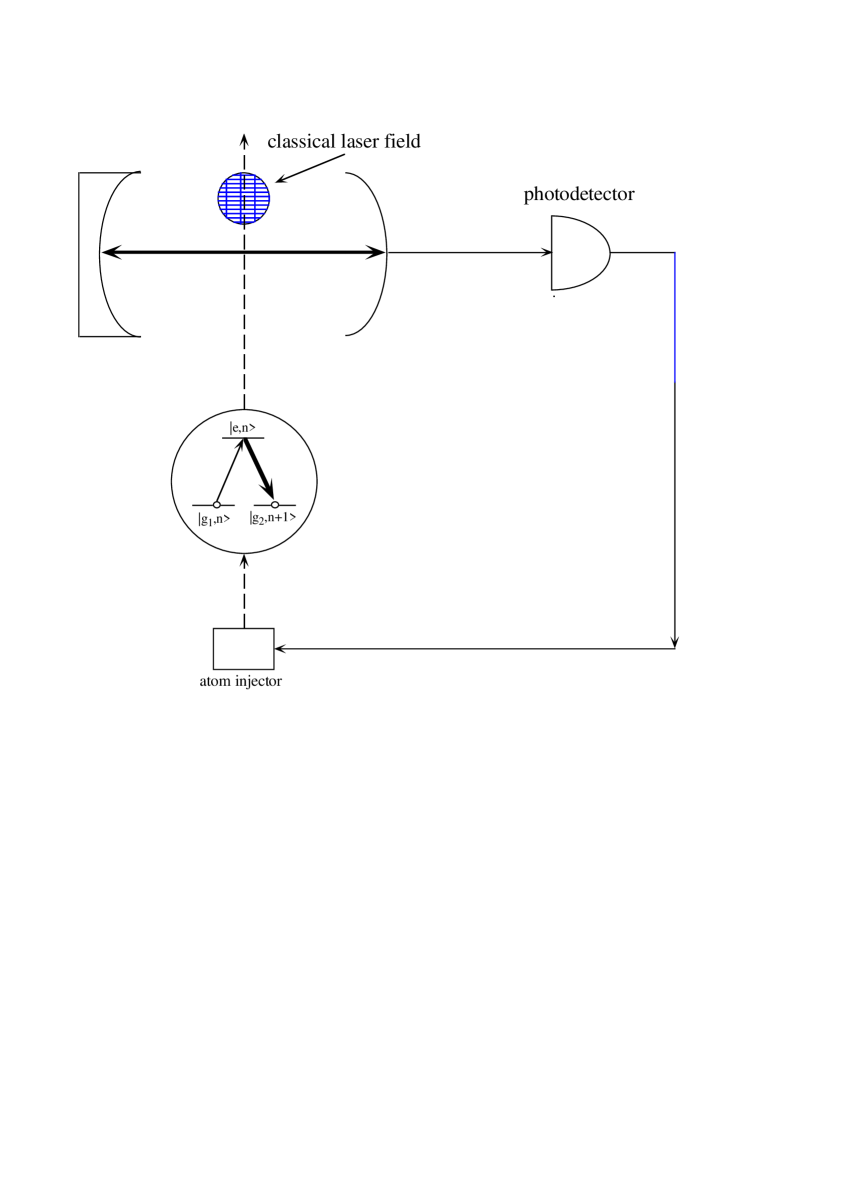
FIG. 1.: Schematic diagram of the photodetection-mediated feedback scheme proposed for optical cavities, together with the appropriate atomic configuration for the adiabatic transfer.

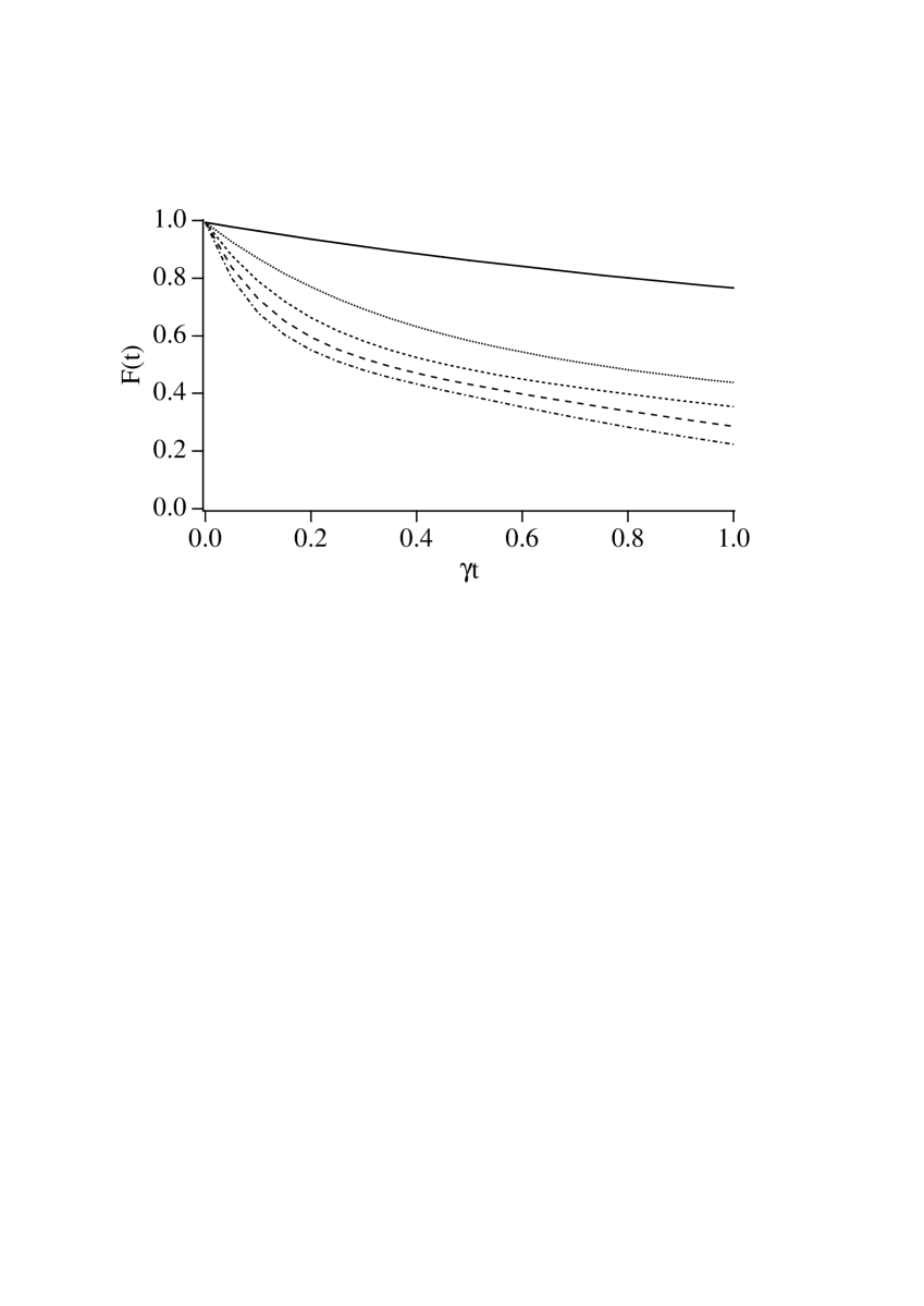
FIG. 2.: Time evolution of the fidelity $F(t)$ for an initial odd cat state with $|\alpha|^{2}=5$; full line: $\eta=1$; dotted line: $\eta=0.75$; small dashes: $\eta=0.5$; big dashes: $\eta=0.25$; dot-dashed line: evolution in absence of feedback ($\eta=0$).

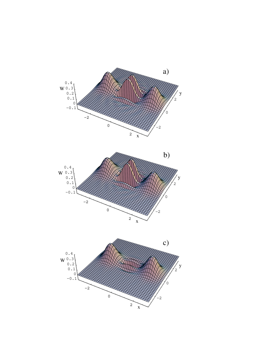
FIG. 3.: (a) Wigner function of the initial odd cat state, $|\psi\rangle=N_{-}(|\alpha\rangle-|-\alpha\rangle)$, $|\alpha|^{2}=5$; (b) Wigner function of the same cat state evolved for a time $t=0.2/\gamma$ ($t=2t_{dec}$), in the presence of feedback ($\eta=1$); (c) Wigner function of the same state after a time $t=0.2/\gamma$, but evolved in absence of feedback.

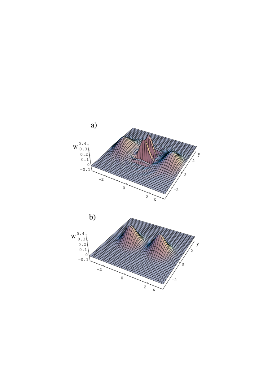
FIG. 4.: Wigner function of the odd cat state of Fig. 3, evolved for a time $t=1/\gamma$ in the presence of ideal feedback $\eta=1$ (a), and in absence of feedback (b).

FIG. 5.: Time evolution of the fidelity $F(t)$ for the initial superposition state of two Fock states $(|2\rangle+2^{1/2}|4\rangle)/3^{1/2}$; full line: $\eta=1$; dotted line: $\eta=0.75$; small dashes: $\eta=0.5$; big dashes: $\eta=0.25$; dot-dashed line: evolution in absence of feedback ($\eta=0$).

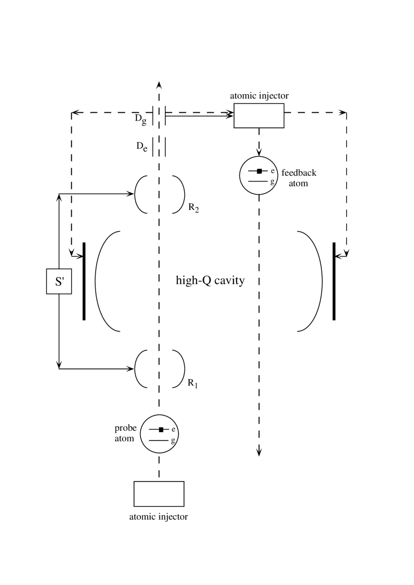
FIG. 6.: Schematic diagram of the stroboscopic feedback scheme for the experiment of Brune et al. $R_{1}$ and $R_{2}$ are the two cavities in which classical microwave pulses can be applied. The feedback loop acts whenever the $g$-state detector clicks and it switches on both the atomic injector and the electric field in the high-Q cavity to Stark-shift the level $e$ into resonance.

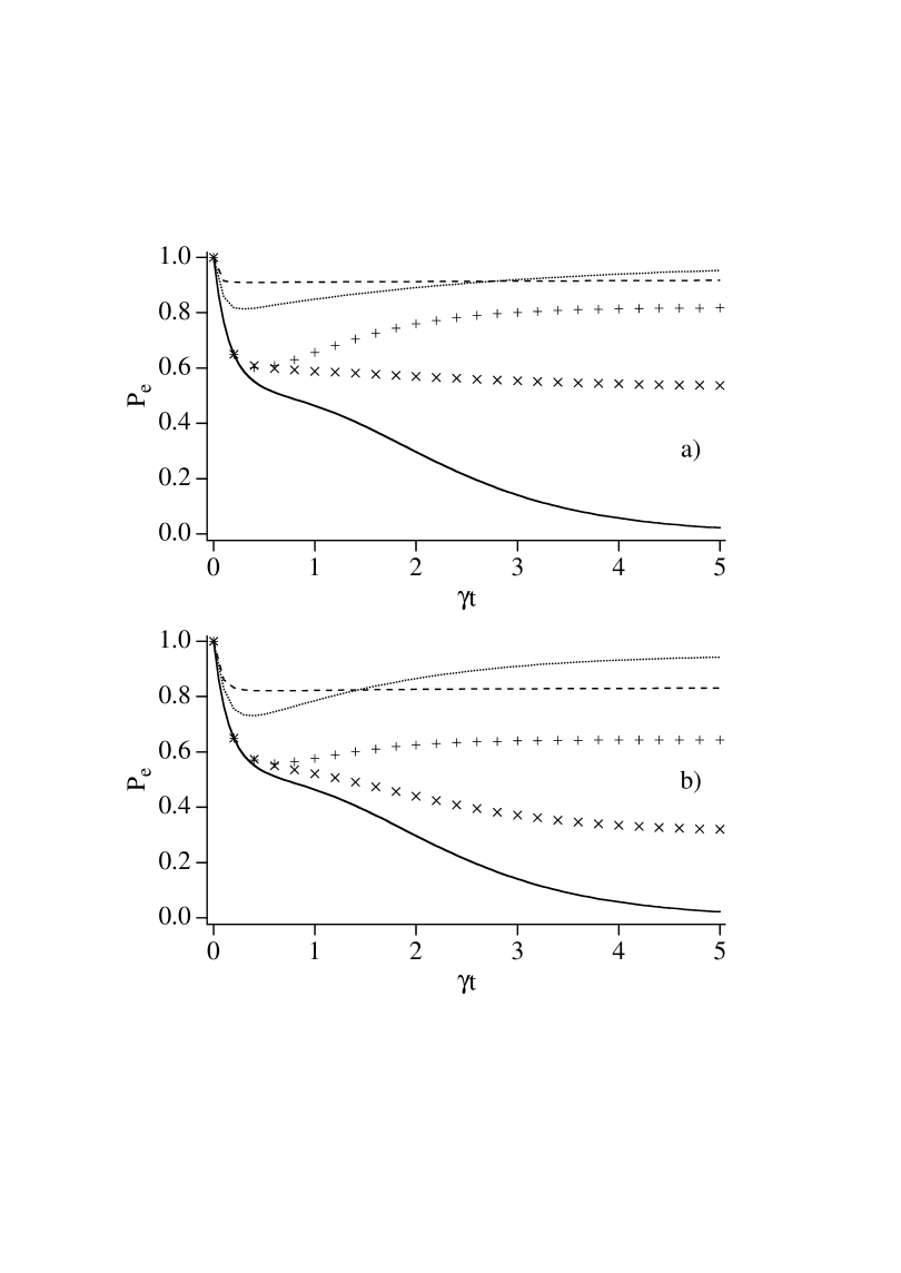
FIG. 7.: Time evolution of the probability of detecting the off-resonant atoms in the state $e$ in the case when $|\alpha|^{2}=3.3$. Full line: $\mu=0$ (no feedback case); dashed line: $\mu=\pi/6$ and $\gamma T=0.02$; dotted line: $\mu=\pi/2$ and $\gamma T=0.02$; horizontal crosses: $\mu=\pi/2$ and $\gamma T=0.2$; diagonal crosses: $\mu=\pi/6$ and $\gamma T=0.2$. In a) the ideal case of perfect atomic detection is considered, while b) refers to the case $\eta=0.4$

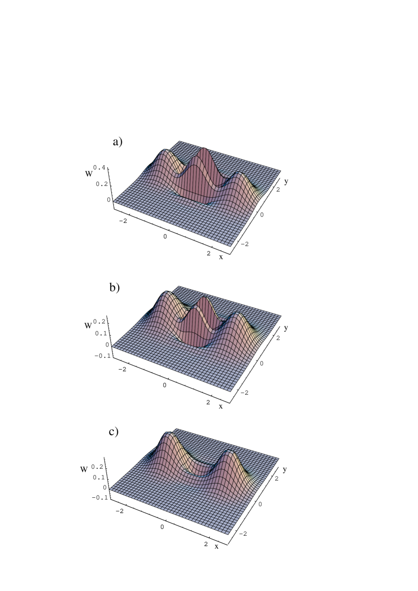
FIG. 8.: (a) Wigner function of the initial odd cat state, $|\psi\rangle=N_{-}(|\alpha\rangle-|-\alpha\rangle)$, $|\alpha|^{2}=3.3$ (b) Wigner function of the same cat state evolved for a time $t=0.44/\gamma$ ($t\sim 3t_{dec}$), in the presence of feedback ($\mu=\pi/6$, $\gamma T=0.02$, $\eta=0.4$); (c) Wigner function of the same state after a time $t=0.44/\gamma$, but evolved in absence of feedback.

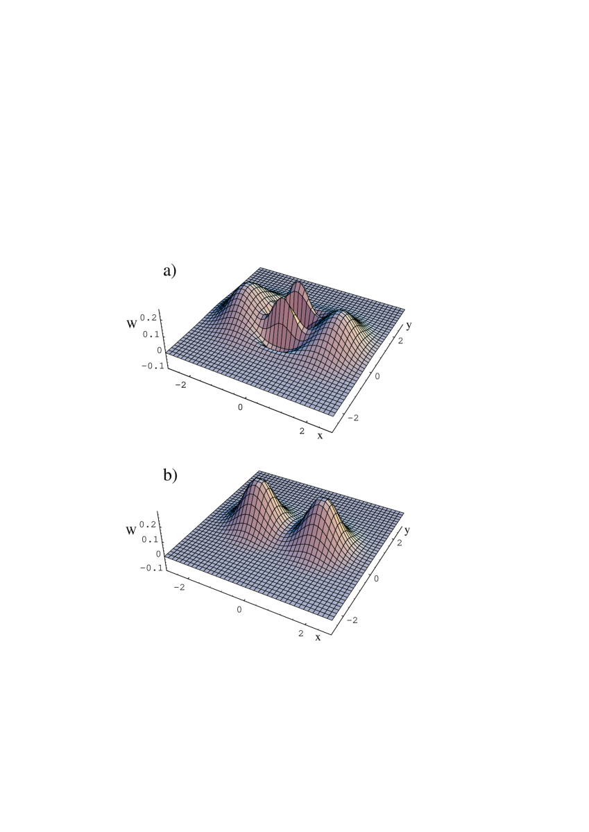
FIG. 9.: Wigner function of the odd cat state of Fig. 8, evolved for a time $t=1/\gamma$ in the presence of feedback with the same parameters as Fig. 8b (a), and in absence of feedback (b).

REFERENCES

- [1] C.H. Bennett, in Quantum Communication, Computing and Measurement, edited by O. Hirota, A.S. Holevo and C.M. Caves (Plenum Press, New York, 1997), pag. 25.
- [2] A. Ekert and R. Josza, Rev. Mod. Phys 68, 733 (1996).
- [3] W.H. Zurek, Phys. Today 44(10), 36 (1991), and references therein.
- [4] A.J. Leggett, in Chance and Matter (Proceedings, 1986 Les Houches Summer School), ed. by J. Souletie, J. Vannimenus, and R. Stora, (North Holland, Amsterdam, 1987), pag. 395.
- [5] Q.A. Turchette, C.J. Hood, W. Lange, H. Mabuchi and H.J. Kimble, Phys. Rev. Lett. 75, 4710 (1995).
- [6] C. Monroe, D.M. Meekhof, B.E. King, W.M. Itano and D.J. Wineland, Phys. Rev. Lett. 75, 4714 (1995).
- [7] E. Schrödinger, Naturwissenschaften 23, 807, 823, 844 (1935).
- [8] A.O. Caldeira and A.J. Leggett, Phys. Rev. A 31, 1059 (1985).
- [9] D.F. Walls and G.J. Milburn, Phys. Rev. A 31, 2403 (1985).
- [10] Quantum Theory and Measurement, ed. by J.A. Wheeler and W.H. Zurek, (Princeton University Press, Princeton NJ, 1983).
- [11] See, e. g. , the debate raised by Zurek’s paper [3] and reported in Phys. Today 46(4), 13 (1993).
- [12] C. Monroe, D.M. Meekhof, B.E. King and D.J. Wineland, Science 272, 1131 (1996).
- [13] M. Brune, E. Hagley, J. Dreyer, X. Maitre, A. Maali, C. Wunderlich, J.M. Raimond and S. Haroche, Phys. Rev. Lett. 77, 4887 (1996).
- [14] D. Vitali, P. Tombesi, G.J. Milburn, Phys. Rev. Lett. 79 2442 (1997).
- [15] D. Vitali, P. Tombesi, G.J. Milburn, J. Mod. Opt. 44 2033 (1997).
- [16] H.M. Wiseman and G.J. Milburn, Phys. Rev. Lett. 70, 548 (1993); Phys. Rev. A 49, 1350 (1994); H.M. Wiseman, Phys. Rev. A 49, 2133 (1994).
- [17] P. Tombesi and D. Vitali, Phys. Rev. A 51, 4913 (1995); P. Goetsch, P. Tombesi and D. Vitali, Phys. Rev. A 54, 4519 (1996).
- [18] H.J. Carmichael, An Open Systems Approach to Quantum Optics, (Springer, Berlin, 1993).
- [19] P. Tombesi and D. Vitali, Phys. Rev. A 50, 4253 (1994).
- [20] C.W. Gardiner, Quantum Noise, (Springer, Berlin, 1991).
- [21] J.F. Poyatos, J.I. Cirac and P. Zoller, Phys. Rev. Lett. 77, 4728 (1996).
- [22] A.S. Parkins, P. Marte, P. Zoller, O. Carnal and H.J. Kimble, Phys. Rev. A 51, 1578 (1995) and references therein.
- [23] A. Messiah, Quantum Mechanics (North Holland, Amsterdam, 1962).
- [24] J.R. Kuklinski, U. Gaubatz, F.T. Hioe and K. Bergmann, Phys. Rev. A 40, 6741 (1990).
- [25] H.M. Wiseman, Phys. Rev. A 51, 2459 (1995).
- [26] C. Wagner, R.J. Brecha, A. Schenzle, and H. Walther, Phys. Rev. A 47, 5068 (1993).
- [27] L. Gilles, B.M. Garraway and P.L. Knight, Phys. Rev. A 49, 2785 (1994).
- [28] K. Vogel, V.M. Akulin and W.P. Schleich, Phys. Rev. Lett. 71, 1816 (1993).
- [29] C.K. Law and J.H. Eberly, Phys. Rev. Lett. 76, 1055 (1996).
- [30] S. Stenholm, Opt. Comm. 123, 287 (1996); P. Törmä and S. Stenholm, Phys. Rev. A 54, 4701 (1996).
- [31] E. Knill and R. Laflamme, Phys. Rev. A 55, 900 (1997) and references therein.
- [32] T. Pellizzari, S.A. Gardiner, J.I. Cirac, and P. Zoller, Phys. Rev. Lett. 75, 3788 (1995).
- [33] H. Mabuchi and P. Zoller, Phys. Rev. Lett, 76, 3108 (1996).
- [34] S. Haroche and J.M. Raymond in Cavity Quantum Electroynamics, P. Berman ed., Academic Press, (1994), p. 123.
- [35] M. Brune, S. Haroche, J.M. Raimond, L. Davidovich and N. Zagury, Phys. Rev. A 45, 5193 (1992).
- [36] L. Davidovich, M. Brune, J.M. Raymond and S. Haroche, Phys. Rev. A 53, 1295 (1996).
- [37] U. Herzog, Phys. Rev. A 53, 1245 (1996).
- [38] C.K. Law and H.J. Kimble, J. Mod. Opt. 44, 2067 (1997).