Decoherence in nonclassical motional states of a trapped ion

Abstract

The decoherence of nonclassical motional states of a trapped ${}^{9}{\rm Be^{+}}$ ion in a recent experiment is investigated theoretically. Sources of decoherence considered here destroy the characteristic coherent quantum dynamics of the system but do not cause energy dissipation. Here they are first introduced phenomenologically and then described using a microscopic Hamiltonian formulation. Theoretical predictions are compared to experimental results.

I Introduction

The experiments of Meekhof et al [1] have revealed quantum dynamics characteristic of the Jaynes-Cummings type (especially collapses and revivals of excitation probabilities) [2] for the first time in a trapped ion system. Stimulated Raman transitions coupled the internal states of a trapped ${}^{9}{\rm Be^{+}}$ ion to its motional states, within the Lamb-Dicke limit of tight ion motion confinement in the trapping potential. The Jaynes-Cummings spin-boson Hamiltonian then derives from the coupling of the internal electronic states of the ion to the vibrational quantum states of motion.

The characteristic quantum dynamics (collapse and revival) of the Jaynes-Cummings type interaction for the ion motion [3, 4, 5] (in the experiment of Meekhof et al [1], an “anti Jaynes-Cummings interaction” for driving the first blue sideband) were observed in the population of the lower atomic state ($P_{\downarrow}$), which was modelled by the phenomenological form fitting the observation as

$$P_{\downarrow}\left(t\right)=\frac{1}{2}\left\{1+\sum_{n}{p_{n}\cos\left(2gt\sqrt{n+1}\right){\rm e}^{-\gamma_{n}t}}\right\}.$$ (1)

Here $p_{n}$ is the initial probability distribution for the motional states in the Fock state basis, $g$ is a coupling constant between the motional states and atomic states (Rabi frequency), and $\gamma_{n}$ is a phenomenological damping rate. The observed damping rate can be written as $\gamma_{n}=\gamma_{0}(n+1)^{\nu}$ with $\nu\approx 0.7$ observed in the experiments of Ref [1]. The damping rate of the $n$th component is independent of that of different components, so that equation (1) implies decoherence without there being transitions between the states of different quantum numbers (energy relaxation). The conventional sources of decoherence, such as spontaneous emission between internal atomic states, and population decay of motional states, cause transitions between the states of different quantum numbers and do not give the decay rate in a form which can be written as $\gamma_{n}$. There have been suggestions [5] as to the origin of this decoherence with the unusual observed value of $\nu$, in terms of decoherence of the ion motion, decoherence of the ion internal levels, and decoherence caused by non-ideal applied fields but the situation has not yet been satisfactorily resolved.

In this paper, we introduce phenomenologically new sources of decoherence, which destroy the characteristic Jaynes-Cummings type dynamics without energy relaxation, by coupling the spin-boson system to a quantum reservoir [6]. The reservoir consists of many-mode bosons described by a canonical distribution at temperature $T$ and introduces noise to the system. We treat decoherence microscopically using a master equation. The master equation coincides with that for stochastic white noise in the high temperature limit of the reservoir under certain approximations (Markovian approximation and ohmic density of states of the reservoir [7]). The advantage of using a quantum boson reservoir is that it not only describes phenomenological quantum noise, but also gives more microscopic information on the source of decoherence, e.g. the noise frequency being responsible for decoherence even in the high temperature limit. Using this combined approach from two directions (phenomenological and microscopic) we discuss the origins of decoherence in this system.

II Description of the system without decoherence

Before investigating decoherence, we consider the system without decoherence, reviewing how the stimulated Raman transitions describe the “anti Jaynes-Cummings” interaction [3, 4, 5] when the first blue sideband is driven, and introducing the dressed states description of the anti Jaynes-Cummings system. We note that the first red sideband driven case (the Jaynes-Cummings interaction case) can be treated just in the same manner, where we exchange the two relevant internal atomic levels $\left|\downarrow\right\rangle$ and $\left|\uparrow\right\rangle$ of the following formulation.

We consider a system with three internal levels $\left|j\right\rangle$ ($j=\underline{0},\downarrow,\uparrow$) and their motional states $\left|n\right\rangle$ ($n=0,1,....$). They are represented by the following Hamiltonian:

$$H_{0}=H_{atom}+H_{vib}$$ (2)

where

$$H_{atom} = -\hbar\omega_{01}|{\downarrow}\rangle\langle{\downarrow}|-\hbar\omega_{02}|{\uparrow}\rangle\langle{\uparrow}|,$$ (3)

$$H_{vib} = \hbar\omega_{x}b^{\dagger}b$$ (4)

with the transition frequency $\omega_{01}$ ($\omega_{02}$) between states $\left|\downarrow\right\rangle$ ($\left|\uparrow\right\rangle$) and $\left|\underline{0}\right\rangle$, the creation (annihilation) operator of the motional states $b^{\dagger}$ ($b$), and the frequency of the motional states $\omega_{x}$. We employ two driving laser beams with detuning $\Delta$, momentum ${\bf k_{1}}$ (${\bf k_{2}}$) and frequency $\omega_{1}$ ($\omega_{2}$) which cause dipole transitions between the level $\left|\downarrow\right\rangle$ ($\left|\uparrow\right\rangle$) and $\left|\underline{0}\right\rangle$. (See Fig. 1) These beams can be treated classically, so the interaction Hamiltonian is

$$H_{int}=-\mbox{\boldmath$\mu$}_{01}\cdot{\rm Re}\left[{\bf E}_{01}{\rm e}^{i\left({\bf k}_{1}\cdot{\bf r}-\omega_{1}t\right)}\right]$$ (5)

$$-\mbox{\boldmath$\mu$}_{02}\cdot{\rm Re}\left[{\bf E}_{02}{\rm e}^{i\left({\bf k}_{2}\cdot{\bf r}-\omega_{2}t\right)}\right]$$ (6)

where $\mbox{\boldmath$\mu$}_{01}$ ($\mbox{\boldmath$\mu$}_{02}$) is the dipole matrix element between $\left|\downarrow\right\rangle$ ($\left|\uparrow\right\rangle$) and $\left|\underline{0}\right\rangle$.

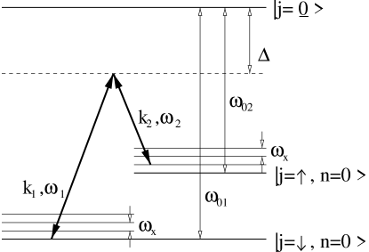
FIG. 1.: Energy levels of the internal states and the motional states.

We apply the rotating wave approximation to the interaction Hamiltonian (6), transform to the interaction picture ($H_{int}^{I}={\rm e}^{iH_{0}t/\hbar}H_{int}{\rm e}^{-iH_{0}t/\hbar}$) and expand in terms of the motional state quantum numbers. When the blue sideband is driven, we have

$$H_{int}^{I} = -\hbar\sum_{n,m}{g_{01}{\rm e}^{i\left\{\left(n-m\right)\omega_{x}+\mit\Delta\right\}t}\left\langle{n}\right|{\rm e}^{i{\bf k}_{1}\cdot{\bf r}}\left|{m}\right\rangle\left|{n}\right\rangle\left\langle{m}\right|\sigma_{1}^{+}}$$ (7)

$$- \hbar\sum_{n,m}{g_{02}{\rm e}^{i\left\{\left(n-m+1\right)\omega_{x}+\mit\Delta\right\}t}\left\langle{n}\right|{\rm e}^{i{\bf k}_{2}\cdot{\bf r}}\left|{m}\right\rangle\left|{n}\right\rangle\left\langle{m}\right|\sigma_{2}^{+}}$$ (8)

$$- h.c.$$ (9)

where we have introduced the dipole operators $\sigma_{1}^{+}\equiv\left|{\underline{0}}\right\rangle\left\langle{\downarrow}\right|$, $\sigma_{2}^{+}\equiv\left|{\underline{0}}\right\rangle\left\langle{\uparrow}\right|$, and the quantities $g_{01}\equiv\mbox{\boldmath$\mu$}_{01}\cdot{\bf E}_{01}/2\hbar$, $g_{02}\equiv\mbox{\boldmath$\mu$}_{02}\cdot{\bf E}_{02}/2\hbar$.

The large detuning condition allows the adiabatic elimination of the level $\left|\underline{0}\right\rangle$ [8]. Under this condition, Raman transitions dominate the system. We also assume the system is cool enough to reach the Lamb-Dicke limit (${\bf k}_{j^{\prime}}\cdot{\bf r}\ll 1$) so we can expand

$${\rm e}^{i{\bf k}_{j^{\prime}}\cdot{\bf r}}\approx 1+ik_{j^{\prime}x}x_{0}\left(b+b^{\dagger}\right),$$ (10)

where $j^{\prime}=1,2$, $x_{0}\equiv\left(\hbar/2m\omega_{x}\right)^{1/2}$ and $m$ is the mass of the ion. Then the effective Hamiltonian in the interaction picture can be written

$$H_{int}^{I}=\hbar\Delta_{1}\left|\downarrow\right\rangle\left\langle\downarrow\right|+\hbar\Delta_{2}\left|\uparrow\right\rangle\left\langle\uparrow\right|$$ (11)

$$+\hbar gb^{\dagger}\left|\uparrow\right\rangle\left\langle\downarrow\right|+\hbar g^{*}b\left|\downarrow\right\rangle\left\langle\uparrow\right|$$ (12)

where $\Delta_{l}\equiv\left|g_{0l}\right|^{2}/\mit\Delta$ and $g\equiv ig_{01}^{*}g_{02}\delta k_{x}x_{0}/\mit\Delta$ with $\delta k_{x}=k_{2x}-k_{1x}$. If we write $S_{+}\equiv\left|\uparrow\right\rangle\left\langle\downarrow\right|$, $S_{-}\equiv\left|\downarrow\right\rangle\left\langle\uparrow\right|$, remove the terms for energy shifts and set $g=g^{*}$, the effective Hamiltonian has the anti Jaynes-Cummings form

$$H_{eff}^{I}=\hbar g\left(b^{\dagger}S_{+}+bS_{-}\right).$$ (13)

This effective Hamiltonian (13) is the origin of the characteristic quantum dynamics (Rabi oscillations, collapses and revivals) of the system. Decoherence is the decay of the off-diagonal elements which represent the characteristic quantum dynamics, so we can use this Hamiltonian to explore some of the sources of decoherence in this interaction picture in the next section.

When working in the interaction picture, it is convenient to introduce the dressed states for the effective Hamiltonian (13):

$$\left|{\varphi\left(n,1\right)}\right\rangle=\frac{1}{\sqrt{2}}\left(\left|{\downarrow,n}\right\rangle+\left|{\uparrow,n+1}\right\rangle\right),$$ (14)

$$\left|{\varphi\left(n,2\right)}\right\rangle=\frac{1}{\sqrt{2}}\left(\left|{\downarrow,n}\right\rangle-\left|{\uparrow,n+1}\right\rangle\right)$$ (15)

$$\left|{\uparrow,0}\right\rangle,$$ (16)

which are the eigenstates of the effective Hamiltonian. We write the eigenvalue of (14) as $E_{+}^{n}$, of (15) as $E_{-}^{n}$, of (16) as $E_{0}$, so we have $E_{\pm}^{n}=\pm\hbar g\sqrt{n+1}$ and $E_{0}=0$. We write the reduced density operator in the dressed state basis as

$$\rho^{I}\left(t\right) = \sum_{n,\alpha}{\sum_{m,\beta}{\rho_{\alpha\beta}^{nm}\left(t\right)}}\left|{\varphi\left(m,\beta\right)}\right\rangle\left\langle{\varphi\left(n,\alpha\right)}\right|$$ (17)

$$+ \sum_{n,\alpha}{\rho_{\alpha 0}^{n}\left(t\right)}\left|{\uparrow,0}\right\rangle\left\langle{\varphi\left(n,\alpha\right)}\right|$$ (18)

$$+ \sum_{m,\beta}{\rho_{0\beta}^{~{}m}\left(t\right)}\left|{\varphi\left(m,\beta\right)}\right\rangle\left\langle{\uparrow,0}\right|$$ (19)

$$+ \rho_{00}\left(t\right)\left|{\uparrow,0}\right\rangle\left\langle{\uparrow,0}\right|$$ (20)

for the boson quantum numbers $n,m=0,1,2,...$ and the spin quantum numbers $\alpha,\beta=1,2$, where $\rho_{\alpha\beta}^{nm}$, $\rho_{\alpha 0}^{n}$,$\rho_{0\beta}^{~{}m}$, $\rho_{00}$ are matrix elements. Then the population of the lower atomic state $P_{\downarrow}$ is

$$P_{\downarrow}\left(t\right)=\frac{1}{2}\left(1-\rho_{00}\left(t\right)+2\sum_{n}{{\rm Re}\left[\rho^{nn}_{12}\left(t\right)\right]}\right).$$ (21)

Note that only the elements that are off-diagonal in terms of the spin quantum number ($\rho^{nn}_{12}\left(t\right)$) and one diagonal element ($\rho_{00}\left(t\right)$) contribute to $P_{\downarrow}$ in the dressed state basis. Basically, the characteristic quantum dynamics observable in the population of the lower state are due to the dynamics of elements that are off-diagonal in terms of the spin quantum number.

III Decoherence without energy relaxation

We next consider the system with the effective Hamiltonian (13) described in the previous section now surrounded by the environment, that is, as an open system. Noise from the environment causes decoherence [9, 10]. We treat this open system by coupling to a quantum reservoir, which consists of an infinite number of many mode bosons

$$H_{r}=\hbar\sum_{l}\omega_{l}B_{l}^{\dagger}B_{l},$$ (22)

where $\omega_{l}$ is the $l$th reservoir frequency, $B_{l}^{\dagger}$ and $B_{l}$ are the creation and annihilation operators of the reservoir bosons. Since the reservoir has infinitely greater degrees of freedom, the reservoir bosons are not affected by the system. Then the time evolution of the reservoir boson operators are given by

$$B_{l}^{\dagger}\left(t\right)={\rm e}^{iH_{r}t/\hbar}B_{l}^{\dagger}{\rm e}^{-iH_{r}t/\hbar}={\rm e}^{i\omega_{l}t}B_{l}^{\dagger},$$ (23)

$$B_{l}\left(t\right)={\rm e}^{iH_{r}t/\hbar}B_{l}{\rm e}^{-iH_{r}t/\hbar}={\rm e}^{-i\omega_{l}t}B_{l}.$$ (24)

The system-reservoir coupling Hamiltonian is

$$H_{sr}=\hbar\sum_{s}{C_{s}}\sum_{l}{g_{sl}\left(B_{l}^{\dagger}+B_{l}\right)}$$ (25)

where $g_{sl}$ is the coupling between a system operator $C_{s}$ and the $l$th reservoir mode. The sum of the system operators $\sum_{s}{C_{s}}$ has to be Hermitian. In the master equation derived from the system-reservoir coupling (25), the damping term consists of the system operators coupling to the reservoir operators. Thus the choice of the coupling between system operators and the reservoir determines the effect of the reservoir. If we choose a system operator $C_{s}$ with the property

$$C_{s}\left|{\varphi\left(n,\alpha\right)}\right\rangle=\sum_{\beta}{c_{\beta}}\left|{\varphi\left(n,\beta\right)}\right\rangle$$ (26)

the resulting master equation describes relaxation within the dressed states of the quantum number $n$, but not energy relaxation between states with different $n$. This is because the time evolution of the density matrix elements in terms of $\left|{\varphi\left(n,\alpha\right)}\right\rangle$ decouples for different $n$. The operators $S_{z}$, $b^{\dagger}b$ are obviously of this type, as these operators do not even change the motional states $\left|n\right\rangle$ as well as the dressed state label $n$. The operator $b^{\dagger}S_{+}+bS_{-}$ changes the motional state, but this operator does not change the dressed state occupation label $n$, so $b^{\dagger}S_{+}+bS_{-}$ is of this type, too. On the other hand, if we choose $C_{s}$ with

$$C_{s}\left|{\varphi\left(n,\alpha\right)}\right\rangle=\sum_{\beta}{c_{\beta}^{\prime}}\left|{\varphi\left(m\neq n,\beta\right)}\right\rangle,$$ (27)

then the resulting master equation describes transitions between states with different boson quantum numbers, which cause energy relaxation; $S_{+}+S_{-}$ and $b+b^{\dagger}$ are of this type.

A Imperfect dipole transition

First, we treat the case when the system operator which is coupling to the reservoir is $b^{\dagger}S_{+}+bS_{-}$. This case looks strange at first sight, but we can consider this as the result of imperfect dipole transitions between the level $\left|\underline{0}\right\rangle$ and the level $\left|j\right\rangle$ ($j=\downarrow,\uparrow$) due to fluctuations of the driving laser intensity. We have previously described how phase fluctuations lead to decoherence and the destruction of quantum revivals in the Jaynes-Cummings model [11]. This is one particular realization of “intrinsic decoherence” in which off-diagonal density matrix elements relax without energy relaxation [11, 12]. We note that these earlier results of ours apply to the experiments of Ref. [1] if the source of decoherence is relative phase fluctuations driving the ionic Raman transition. Here we analyse more general sources of decoherence. The imperfect dipole transitions $\left|\downarrow\right\rangle\Leftrightarrow\left|\underline{0}\right\rangle$ and $\left|\uparrow\right\rangle\Leftrightarrow\left|\underline{0}\right\rangle$ are represented by

$$\sigma_{1}^{\pm} \rightarrow \sigma_{1}^{\pm}+\sigma_{1}^{\pm}\sum_{l}{g_{l}\left(B_{l}^{\dagger}+B_{l}\right)},$$ (28)

$$\sigma_{2}^{\pm} \rightarrow \sigma_{2}^{\pm}+\sigma_{2}^{\pm}\sum_{l}{g_{l}\left(B_{l}^{\dagger}+B_{l}\right)}.$$ (29)

We assume the system-reservoir coupling is weak enough, so we can neglect the terms that are second order in $g_{l}$. Then we have, for example,

$$S_{+}=\sigma_{2}^{-}\sigma_{1}^{+} \rightarrow \sigma_{2}^{-}\sigma_{1}^{+}+\sigma_{2}^{-}\sigma_{1}^{+}\sum_{l}{g_{l}\left(B_{l}^{\dagger}+B_{l}\right)}.$$ (30)

Thus the Hamiltonian describing the system-reservoir coupling is given by

$$H_{sr} = \hbar\left(b^{\dagger}S_{+}+bS_{-}\right)\sum_{l}{g_{l}^{\prime}\left(B_{l}^{\dagger}+B_{l}\right)}$$ (31)

where $g_{l}^{\prime}=gg_{l}$. This Hamiltonian (31) can be interpreted as if the Rabi frequency ($g$) of the Jaynes-Cummings type system fluctuates due to the system-reservoir coupling as

$$g\rightarrow g+\sum_{l}{{g_{l}}^{\prime}\left(B_{l}+B_{l}^{\dagger}\right)}.$$ (32)

Using a time convolution-less (TCL) formulation (this approach is described in detail in [13]) of the quantum damping theory [9] and the rotating wave approximation on the master equation [14] the master equation in the interaction picture is

$$\frac{\partial}{\partial t}\rho^{I}\left(t\right)=\frac{1}{i\hbar}\left[{H_{eff}^{I},\rho^{I}\left(t\right)}\right]+{\it\Gamma}\rho^{I}\left(t\right)$$ (33)

where the damping term ${\it\Gamma}\rho^{I}$ is given by [15]

$${\it\Gamma}\rho^{I}\left(t\right) = \sum_{l}{{g_{l}^{\prime}}^{2}\int_{0}^{t}{dt^{\prime}\biggl{\{}\left(\langle B_{l}^{\dagger}\left(t^{\prime}\right)B_{l}\rangle_{B}+\langle B_{l}\left(t^{\prime}\right)B_{l}^{\dagger}\rangle_{B}\right)\biggr{.}}}$$ (34)

$$\times \left(\left[\underline{b^{\dagger}S_{+}}\left(-t^{\prime}\right)\rho^{I}\left(t\right),bS_{-}\right]+\left[\underline{bS_{-}}\left(-t^{\prime}\right)\rho^{I}\left(t\right),b^{\dagger}S_{+}\right]\right)$$ (35)

$$+ \left(\langle B_{l}^{\dagger}\left(-t^{\prime}\right)B_{l}\rangle_{B}+\langle B_{l}\left(-t^{\prime}\right)B_{l}^{\dagger}\rangle_{B}\right)$$ (36)

$$\times \biggl{.}\left(\left[b^{\dagger}S_{+},\rho^{I}\left(t\right)\underline{bS_{-}}\left(-t^{\prime}\right)\right]+\left[bS_{-},\rho^{I}\left(t\right)\underline{b^{\dagger}S_{+}}\left(-t^{\prime}\right)\right]\right)\biggr{\}}$$ (37)

with

$$\underline{b^{\dagger}S_{+}}(t)={\rm e}^{iH_{eff}^{I}t/\hbar}b^{\dagger}S_{+}{\rm e}^{-iH_{eff}^{I}t/\hbar},$$ (38)

$$\underline{bS_{-}}(t)={\rm e}^{iH_{eff}^{I}t/\hbar}bS_{-}{\rm e}^{-iH_{eff}^{I}t/\hbar}.$$ (39)

The master equation (33) can be solved by expanding all system operators in terms of the dressed states under certain reservoir conditions. We require the reservoir to be the canonical distribution at temperature $T$ and the time scale of the reservoir variables to be much shorter than the system variables so we can take the Markovian limit.

We take the continuum limit of the reservoir modes,

$$\sum_{l}\rightarrow\int{d\omega D(\omega)}$$ (40)

where $D(\omega)$ is the density of states of the reservoir. The corresponding continuum expression for $g_{l}$ is $g(\omega)$. The master equation is cast into a group of differential equations for the density matrix elements. The time evolution of density matrix elements having different boson quantum numbers are decoupled due to the character of the coupling between the system operator and the reservoir. The time evolution of the diagonal elements ($\rho_{\alpha\alpha}^{nn}$) and the off-diagonal elements ($\rho_{\alpha\beta}^{nn}$, $\alpha\neq\beta$) having the same boson number ($n$) are also decoupled.

To calculate the time evolution of $P_{\downarrow}$, we only need the elements $\rho_{12}^{nn}$ and $\rho_{00}$. The equations for the time evolution of these elements are

$$\frac{\partial}{\partial t}\rho_{00}\left(t\right) = 0,$$ (41)

$$\frac{\partial}{\partial t}\rho_{12}^{nn}\left(t\right) = -i\Omega_{n}\rho_{12}^{nn}\left(t\right)$$ (42)

$$- \left(n+1\right)\left\{\bar{n}\left(n\right)+1/2\right\}\kappa\left(n\right)\rho_{12}^{nn}\left(t\right)$$ (43)

$$- 2\left(n+1\right)\kappa_{0}\bar{n}_{0}\rho_{12}^{nn}\left(t\right)$$ (44)

$$- \left(n+1\right)\left\{\bar{n}\left(n\right)+1/2\right\}\kappa\left(n\right)\rho_{21}^{nn}\left(t\right),$$ (45)

where

$$\Omega_{n}=E_{n}^{+}-E_{n}^{-}=2g\sqrt{n+1}.$$ (46)

In (45), the function of the reservoir bosons $\bar{n}\left(n\right)$ is

$$\bar{n}\left(n\right)=\left({\rm e}^{\hbar\Omega_{n}/k_{B}T}-1\right)^{-1},$$ (47)

and the damping function $\kappa\left(n\right)$ is

$$\kappa\left(n\right)\sim D(\Omega_{n})\cdot g(\Omega_{n}),$$ (48)

which represents the effective contribution of the reservoir bosons having frequency $\Omega_{n}$. So the combination of these ($\kappa\left(n\right)\left\{\bar{n}\left(n\right)+1/2\right\}$) represents the effective mean number of the reservoir bosons with frequency $\Omega_{n}$. The quantity $\kappa_{0}\bar{n}_{0}$ is the contribution from zero frequency reservoir bosons.

The analytical solution of the equation (45) is

$$\rho_{12}^{nn}\left(t\right) = {\rm e}^{-A_{n}t}\left\{\cos\left(B_{n}t\right)-i{\Omega_{n}}/{B_{n}}\sin\left(B_{n}t\right)\right\}\rho_{12}^{nn}\left(0\right)$$ (49)

$$- {\rm e}^{-A_{n}t}{A_{n}}/{B_{n}}\sin\left(B_{n}t\right)\rho_{21}^{nn}\left(0\right)$$ (50)

where

$$A_{n} = \left(n+1\right)\kappa\left(n\right)\left\{\bar{n}\left(n\right)+1/2\right\}+2\left(n+1\right)\kappa_{0}\bar{n}_{0}$$ (51)

$$\equiv A_{n}^{dipole},$$ (52)

$$B_{n} = \sqrt{\Omega_{n}^{2}-A_{n}^{2}}.$$ (53)

With the chosen initial condition: $|\downarrow\rangle\langle\downarrow|$ for the atom and $\sum_{n}p_{n}|n\rangle\langle n|$ for the motional state, the real part of Eq. (50) is found to be

$${\rm Re}\left[\rho_{12}^{nn}\left(t\right)\right]=\frac{{\rm e}^{-A_{n}t}}{2}\sqrt{1+\left(\frac{A_{n}}{B_{n}}\right)^{2}}\cos\left(B_{n}t+\theta_{n}\right)$$ (54)

where $\theta_{n}$ is a phase shift defined by $\theta_{n}=\arctan\left(A_{n}/B_{n}\right)$. Thus we see that the damping rate $A_{n}$ depends on the effective mean number of the reservoir bosons with frequency $\Omega_{n}$, with a factor $n+1$. The coupling to the reservoir also shifts the oscillation from $\Omega_{n}t$ to $B_{n}t+\theta_{n}$. Since we assumed that the system-reservoir coupling is weak in our formulation, $\kappa\left(n\right)$ in $A_{n}$ must be much smaller than the Rabi frequency $g$. Thus we have relation $A_{n}\ll B_{n}\sim\Omega_{n}$. Under this condition, the population of the lower atomic state $P_{\downarrow}$ is approximated to be

$$P_{\downarrow}\left(t\right)=\frac{1}{2}\left\{1+\sum_{n}{p_{n}\cos\left(\Omega_{n}t\right){\rm e}^{-A_{n}t}}\right\},$$ (55)

which is in the same form as that seen in the experiments [1].

B Fluctuation of vibrational potential

Next, we consider the case that the system couples to the reservoir via the system operator $b^{\dagger}b$. The system-reservoir coupling Hamiltonian is

$$H_{sr}=\hbar b^{\dagger}b\sum_{l}{g_{l}^{\prime}\left(B_{l}^{\dagger}+B_{l}\right)}.$$ (56)

This coupling describes fluctuations of the trap potential. Then the damping term is

$${\it\Gamma}\rho^{I}\left(t\right) = \sum_{l}{{g_{l}^{\prime}}^{2}\int_{0}^{t}{dt^{\prime}\biggl{\{}\left(\langle B_{l}^{\dagger}\left(t^{\prime}\right)B_{l}\rangle_{B}+\langle B_{l}\left(t^{\prime}\right)B_{l}^{\dagger}\rangle_{B}\right)\biggr{.}}}\$$ (57)

$$\times \left[b^{\dagger}b\left(-t^{\prime}\right)\rho^{I}\left(t\right),b^{\dagger}b\right]$$ (58)

$$+ \left(\langle B_{l}^{\dagger}\left(-t^{\prime}\right)B_{l}\rangle_{B}+\langle B_{l}\left(-t^{\prime}\right)B_{l}^{\dagger}\rangle_{B}\right)$$ (59)

$$\times \biggl{.}\left[b^{\dagger}b,\rho^{I}\left(t\right)b^{\dagger}b\left(-t^{\prime}\right)\right]\biggr{\}}$$ (60)

where

$$b^{\dagger}b\left(t\right)={\rm e}^{iH^{I}_{eff}t/\hbar}b^{\dagger}b\/{\rm e}^{-iH^{I}_{eff}t/\hbar}.$$ (61)

After expanding (60) in terms of the dressed states, the time evolution of $\rho_{12}^{nn}$ and $\rho_{00}$ are

$$\frac{\partial}{\partial t}\rho_{00}\left(t\right) = 0,$$ (62)

$$\frac{\partial}{\partial t}\rho_{12}^{nn}\left(t\right) = -i\Omega_{n}\rho_{12}^{nn}\left(t\right)$$ (63)

$$- \frac{1}{2}\left\{\bar{n}\left(n\right)+1/2\right\}\kappa\left(n\right)\rho_{12}^{nn}\left(t\right)$$ (64)

$$+ \frac{1}{2}\left\{\bar{n}\left(n\right)+1/2\right\}\kappa\left(n\right)\rho_{21}^{nn}\left(t\right).$$ (65)

The analytical solution of ${\rm Re}\left[\rho_{12}^{nn}\right]$ is given by (54) with

$$A_{n}=\frac{1}{2}\kappa\left(n\right)\left\{\bar{n}\left(n\right)+1/2\right\}\equiv A_{n}^{vib}.$$ (66)

$B_{n}$ is defined by the equation (53). We note that equations (62)-(65) coincide with those for the case of coupling to the reservoir via $S_{z}$ ($H_{sr}=\hbar S_{z}\sum{g_{l}^{\prime}\left(B_{l}^{\dagger}+B_{l}\right)}$).

IV Estimation of reservoir variables

The formulation of the decoherence rates $A_{n}^{dipole}$ (52) and $A_{n}^{vib}$ (66) in the previous section shows that decoherence originates in the relaxation of density matrix elements that are diagonal in the boson quantum number but off-diagonal in the spin quantum numbers in the dressed state basis. The relaxation of the element $\rho_{\alpha\beta}^{nn}$ for $\alpha\neq\beta$ is caused by the coupling to reservoir bosons at frequency of $\Omega_{n}$ ($=2g\sqrt{n+1}$). The effective contribution of reservoir bosons at frequency of $\Omega_{n}$ is therefore the key to understand the decoherence rate.

The Rabi frequency $g$ in the Boulder experiment [1] is around 100 kHz, so reservoir bosons of order $100$ kHz seem to be responsible for decoherence. These reservoir bosons have a much lower frequency than those responsible for the case of spontaneous emission between internal atomic states, which is of order GHz here, and also population decay of motional states, which is of order 10 MHz. This low frequency nature of the reservoir bosons important here suggests that the reservoir may be at non-zero temperature whereas of course in the optical frequency regime, the reservoir is often approximated to be at a zero temperature.

What are these reservoir bosons in the experiment? To consider this question and discuss the origin of decoherence, we investigate the other characteristics, which the reservoir bosons should satisfy, by comparing our theoretical results to the experiment. For this purpose, we introduce normalised values, $\tilde{A}_{n}^{dipole}=A_{n}^{dipole}/g$, $\tilde{A}_{n}^{vib}=A_{n}^{vib}/g$, $\tilde{\omega}_{x}=\omega_{x}/g$, $\tilde{T}=k_{B}T/\hbar g$, $\tilde{\Omega}_{n}=\Omega_{n}/g$, $\tilde{\gamma}_{0}=\gamma_{0}/g$, $\tilde{\kappa}\left(n\right)=\kappa\left(n\right)/g$. The normalised decoherence rates are

$$\tilde{A}_{n}^{dipole} = \left(n+1\right)\tilde{\kappa}\left(n\right)f\left(n,\tilde{T}\right)+2\left(n+1\right)\kappa_{0}\bar{n}_{0},$$ (67)

$$\tilde{A}_{n}^{vib} = \frac{1}{2}\tilde{\kappa}\left(n\right)f\left(n,\tilde{T}\right)$$ (68)

where

$$f\left(n,\tilde{T}\right)=\bar{n}\left(n\right)+\frac{1}{2}=\frac{1}{2}\coth\frac{\sqrt{n+1}}{\tilde{T}}.$$ (69)

The experimentally observed decoherence rate can be written as $\tilde{A}_{n}^{ex}=\tilde{\gamma}_{0}\left(n+1\right)^{\nu}$. In the experiment, $g/2\pi=94$ kHz, $\gamma_{0}=11.9$ kHz, so we have $\tilde{\gamma}_{0}=0.127/2\pi$.

Let us further assume that $\tilde{\kappa}\left(n\right)$ described by (48) is given by a power $d$ of the frequency $\tilde{\Omega}_{n}$ [7],

$$\tilde{\kappa}\left(n\right)=\tilde{a}\tilde{\Omega}_{n}^{d}=\tilde{a}\left(2\sqrt{n+1}\right)^{d}$$ (70)

where $\tilde{a}$ is a damping constant ($\tilde{a}\ll 1$). Some high frequency cut-off of the damping function is assumed to prevent divergence. These are the usual arguments given for the reservoir density of states. Generally, the case of $d=1$ is known as the Ohmic case, since the choice of $d$ gives a velocity dependent dissipation rate for the dissipative two-state system [7], and $d=3$ is required to describe 3-D radiation fields [16]. However, we do not restrict ourselves to $d$ as an integer. We ignore the effect of zero frequency reservoir bosons: $\kappa_{0}\bar{n}_{0}=0$.

The decoherence rates at $n=0$ have to coincide with $\tilde{\gamma}_{0}$. So we have $\tilde{\gamma}_{0}=\tilde{\kappa}(0)f(0,\tilde{T})$ for the imperfect dipole transition case and $\tilde{\gamma}_{0}=\tilde{\kappa}(0)f(0,\tilde{T})/2$ for the case of fluctuations of the vibrational potential. These conditions for $\tilde{\gamma}_{0}$ determine $\tilde{a}$ when the value of $\tilde{\gamma}_{0}$ is given. Thus the decoherence rate is rewritten as

$$\tilde{A}_{n}^{dipole} = \tilde{\gamma}_{0}\left(n+1\right)^{1+d/2}f\left(n,\tilde{T}\right)/f\left(0,\tilde{T}\right),$$ (71)

$$\tilde{A}_{n}^{vib} = \tilde{\gamma}_{0}\left(n+1\right)^{d/2}f\left(n,\tilde{T}\right)/f\left(0,\tilde{T}\right).$$ (72)

The remaining unrestricted fitting parameters in our formulation are the normalised temperature $\tilde{T}$ and the power dependency $d$ in Eq.(47). The value $f\left(0,\tilde{T}\right)/f\left(n,\tilde{T}\right)$ lies in the range

$$\left(1+n\right)^{-1/2}\leq f\left(n,\tilde{T}\right)/f\left(0,\tilde{T}\right)\leq 1.$$ (73)

We take the high temperature limit ($\tilde{T}\rightarrow\infty$). This limit represents classical noise where the reservoir operators commute $\left(\left[B_{l},B_{l}^{\dagger}\right]=0\right)$. The value $f\left(n,\tilde{T}\right)/f\left(0,\tilde{T}\right)$ becomes $\left(n+1\right)^{-1/2}$ when $\tilde{T}\rightarrow\infty$, so we have

$$\tilde{A}_{n}^{dipole} = \tilde{\gamma}_{0}\left(n+1\right)^{(d+1)/2}$$ (74)

$$\tilde{A}_{n}^{vib} = \tilde{\gamma}_{0}\left(n+1\right)^{(d-1)/2}.$$ (75)

The linear form $\tilde{\gamma}_{0}\left(n+1\right)$ is reached for $d=1$ (the Ohmic case) for the imperfect dipole transition and for $d=3$ (3-D radiation field) for the case of fluctuations of the vibrational potential. To get a power exponent of $0.7$ for $n+1$ we need $d\approx 0.4$ for the imperfect dipole transition case (Fig. 2) and $d\approx 2.4$ for the case of fluctuations of the vibrational potential.

FIG. 2.: The population of the lower atomic state $P_{\downarrow}\left(t\right)$ against the normalised time $gt/2\pi$ when (1) the initial internal state is $\left|\downarrow\right\rangle$ and the initial motional state is a Fock state with condition $\left|1\right\rangle$; (2) the initial motional state is a coherent state with condition $\left|\alpha=3.0\right\rangle$. For both figures, the dashed lines are for the case of no decoherence and the solid lines are for the case of an imperfect dipole transition with the coefficients $d=0.4$ and ${\tilde{\gamma}}_{0}=0.127/2\pi$ in the high temperature limit $\tilde{T}\rightarrow\infty$.

V Summary and open questions

In summary, we have shown here a model describing decoherence which destroys the characteristic quantum dynamics (collapse and revival) of the Jaynes-Cummings system without energy relaxation for the ion trap experiment [1]. The sources of decoherence are first introduced phenomenologically and then described by a master equation using a microscopic Hamilton formulation. We apply the model to the two possible actual sources of decoherence; one is the imperfect dipole transition, and the other is the fluctuation of vibrational potential. We solve the master equation under the Markovian approximation and continuum limit of the reservoir modes.

The analytical solution shows that decoherence is described by the reservoir bosons with frequency $\Omega_{n}=2g\sqrt{n+1}$. Therefore, the effective contribution of the bosons at frequency of $\Omega_{n}$ (which is of order 100 kHz) was found to be the key to understand the decoherence. This low frequency nature of the reservoir bosons compared to the spontaneous emission transition frequencies (which are of order GHz) and population decay transition frequencies (which is of order 10 MHz) suggests that the reservoir may be regarded to be at non-zero temperature. If we assume the high temperature limit and certain density of states of the reservoir bosons, the decay rate coincides with that seen in the experiment [1].

To proceed further and investigate the origin of decoherence for the Boulder ion trap experiment [1], we would have to know a number of parameters:

1. The intensity fluctuations of the dye laser used for the stimulated Raman transition which seems to be order of $10^{5}$-$10^{6}$ Hz, so this may well be a candidate for the fluctuation affecting the bosons. But we would need to know more about the frequency dependence of the intensity fluctuation around 100 kHz to take the analysis much further.

2. Noise from the trap potential from the radio frequency (100-200 kHz) radiation field is possible, but again we would need to estimate the density of states for this case to be more precise.

3. Possibility of quantum noise (noise at finite $T$) remains a potential candidate to explain this decoherence.

We defer further consideration of all these until the underlying parameters are better understood. Since this paper was submitted for publication we learnt of related work by Schneider and Milburn [17], and by James [18].

REFERENCES

• [1] D.M. Meekhof, C. Monroe, B.E. King, W.M. Itano and D.J. Wineland, Phys. Rev. Lett. 76, 1796 (1996).
• [2] B.W. Shore and P.L. Knight, J. Mod. Opt. 40 (1993) 1195.
• [3] C.A. Blockley, D.F. Walls and H. Risken, Europhys. Lett. 17 (1992) 509; W. Vogel and R.L. De Matos Filho, Phys. Rev. A 49 (1995) 4214; J.I. Cirac, R. Blatt, A.S. Parkins and P. Zoller, Phys. Rev. A 49 (1994) 1202.
• [4] D. Leibfried, D.M. Meekhof, C. Monroe, B.E. King, W.M. Itano and D.J. Wineland, J. Mod. Opt 44 (1997) 2485 and references therein.
• [5] D.J. Wineland, C. Monroe, W.M. Itano, D. Leibfried, B. King and D.M. Meekhof, submitted to Rev. Mod. Phys. (1997).
• [6] S. Bose, P.L. Knight, M. Murao, M.B. Plenio and V. Vedral, Phil. Trans. R. Soc. (in press), (1998).
• [7] A.J. Leggett, S. Chakaravary, A.T. Dorsey, M.P.A. Fisher, A. Garg and W. Zwerger, Rev. Mod. Phys. 59 (1987) 1.
• [8] J. Steinbach, J. Twamley, and P.L. Knight, Phys. Rev. A 56 (1997) 4815.
• [9] W.E. Louisell, Quantum Statistical Properties of Radiation (John Wiley & Sons, Inc., New York, 1973).
• [10] W.H. Zurek, Phys. Today 44 (1991) 36.
• [11] H. Moya-Cessa, V. Bu$\check{z}$ek, M.S. Kim and P.L. Knight, Phys. Rev. A. 48 (1993) 3900.
• [12] G.J. Milburn, Phys. Rev. A 44 (1991) 5401.
• [13] F. Shibata and T. Arimitsu, J. Phys. Soc. Jpn 49 (1980) 891.
• [14] M. Murao, J. Phys. Soc. Jpn. 66 (1997) 2314.
• [15] M. Murao and F. Shibata, J. Phys. Soc. Jpn. 64 (1995) 2394.
• [16] C.H. Keitel, P.L.Knight, L.M. Marducci and M.O. Scully, Opt. Commun. 118 (1995) 143.
• [17] S. Schneider and G.J. Milburn, quant-ph/9710044.
• [18] D.F.V. James, The thoery of heating of the quantum ground state of trapped ions, submitted for publication.