Local Search Methods for Quantum Computers

Abstract

Local search algorithms use the neighborhood relations among search states and often perform well for a variety of NP-hard combinatorial search problems. This paper shows how quantum computers can also use these neighborhood relations. An example of such a local quantum search is evaluated empirically for the satisfiability (SAT) problem and shown to be particularly effective for highly constrained instances. For problems with an intermediate number of constraints, it is somewhat less effective at exploiting problem structure than incremental quantum methods, in spite of the much smaller search space used by the local method.

1 Introduction

Combinatorial search problems are among the most difficult computational tasks: the time required to solve them often grows exponentially with the size of the problem [16]. Many such problems have a great deal of structure, allowing heuristic methods to greatly reduce the rate of exponential growth. Quantum computers [2, 3, 11, 12, 13, 14, 28] offer a new possibility for utilizing this structure with quantum parallelism, i.e., the ability to operate simultaneously on many classical search states, and interference among different paths through the search space.

While several algorithms have been developed [38, 5, 18, 21, 22], the extent to which quantum searches can improve on heuristically guided classical methods for NP searches remains an open question. Even if quantum computers are not useful for all combinatorial search problems, they may still be useful for many instances encountered in practice. This is an important distinction since typical instances of search problems are often much easier to solve than is suggested by worst case analyses, though even typical costs often grow exponentially on classical machines. The study of the average or typical behavior of search heuristics relies primarily on empirical evaluation. This is because the complicated conditional dependencies in search choices made by the heuristic often preclude a simple theoretical analysis, although phenomenological theories can give an approximate description of some generic behaviors [20, 26, 33].

The simplest algorithms are the unstructured methods, such as generate-and-test, which amount to a random search among the states or a systematic enumeration of them without any use of prior results to guide future choices. An analogous unstructured quantum search can improve on this classical method [18].

One structured approach to search builds solutions incrementally from smaller parts. These methods exploit the fact that in many problems the small parts can be tested for consistency before they are expanded to larger ones. When a small part is found to be inconsistent, all possible extensions of it will also be inconsistent, allowing an early pruning of the search. In such cases, the search backtracks to a prior decision point to try a different incremental construction. Analogies with this approach form the basis of previously proposed structured quantum searches [21, 22].

A second approach takes advantage of the clustering of solutions found in many search problems. That is, instead of being randomly distributed throughout the search space, the states have a simple neighborhood relationship such that states with a few or no conflicts tend to be near other such states. This neighborhood relationship is used by repair or local searches. Starting from a random state, they repeatedly select from among the current state’s neighbors one that reduces the number of conflicts with the constraints. Such searches can become stuck in local minima but are often very effective [32, 36]. The problem of local minima can be addressed by allowing occasional changes that increase the number of conflicts [25]. By comparison with incremental methods, local searches operate in a smaller search space, i.e., they have no need to consider the many small parts that might be composed into a full solution. On the other hand, they also disregard any information from these small parts that can guide the search toward a solution.

In this paper, we present a new quantum search algorithm based on the neighborhood structure of the satisfiability problem. Such structure forms the basis of many local classical methods but has not yet been applied to quantum computation. Specifically the following two sections describe the satisfiability problem used to illustrate our algorithm and the ingredients of quantum programs. We then describe a quantum algorithm analogous to classical local search methods and evaluate its behavior. Finally some open issues are discussed, including a variety of ways this approach can be extended. The appendices derive the properties of the algorithm’s quantum operation and discuss approaches to the classical simulation of the algorithm.

2 The Satisfiability Problem

NP search problems have exponentially many possible states and a procedure that quickly checks whether a given state is a solution [16]. Constraint satisfaction problems (CSPs) [30] are an important example. A CSP consists of $n$ variables, $V_{1},\ldots,V_{n}$, and the requirement to assign a value to each variable to satisfy given constraints. Searches examine various assignments, which give values to some of the variables. Complete assignments have a value for every variable.

One important CSP is the satisfiability problem (SAT), which consists of a propositional formula in $n$ variables and the requirement to find a value (true or false) for each variable that makes the formula true. This problem has $N=2^{n}$ complete assignments. For $k$-SAT, the formula consists of a conjunction of clauses and each clause is a disjunction of $k$ variables, any of which may be negated. For $k\geq 3$ these problems are NP-complete. An example of such a clause for $k=3$, with the third variable negated, is $V_{1}$ OR $V_{2}$ OR $\overline{V_{3}}$, which is false for exactly one assignment for these variables: $\{V_{1}={\rm false},V_{2}={\rm false},V_{3}={\rm true}\}$. With the formula expressed as a conjunction of clauses, a solution must satisfy every clause. Thus we can view each clause as a constraint that adds one conflict to all complete assignments that include assignments to the variables in the clause that make it false. By selecting the clauses to be distinct, the number of clauses $m$ corresponds to the number of constraints in the problem.

The assignments for SAT can also be viewed as bit strings with the correspondence that the $i^{th}$ bit is 0 or 1 according to whether $V_{i}$ is assigned the value false or true, respectively. In turn, these bit strings are the binary representation of integers, ranging from 0 to $2^{n}-1$. For definiteness, we associate the value of variable $V_{i}$ with the bit in the integer corresponding to $2^{i-1}$, i.e., $V_{1}$ corresponds to the least significant bit. Each clause in the a $k$-SAT formula specifies a combination of $k$ bits that cause a conflict in any assignment containing all of them. For example, the clause $V_{1}$ OR $V_{2}$ OR $\overline{V_{3}}$ introduces a conflict in all assignments for which bits 1 and 2 are 0 and bit 3 is 1, i.e., assignments whose integer representation ends with the bit string 100.

For bit strings $r$ and $s$, we define ${|s|}$ to be the number of 1-bits in $s$ and $r\wedge s$ to be the bitwise AND operation on $r$ and $s$. Thus ${|r\wedge s|}$ counts the number of 1-bits both assignments have in common, and can also be viewed as a bitwise dot product of the two assignments considered as vectors of bits. We also use $d(r,s)$ as the Hamming distance between $r$ and $s$, i.e., the number of positions at which they have different values. These quantities are related by

$$d(r,s)={|r|}+{|s|}-2{|r\wedge s|}$$ (1)

An example with $n=2$ and two constraints, each involving a single variable, is $V_{1}\neq 1$ and $V_{2}\neq 1$. This problem has a unique solution: $V_{1}=0,V_{2}=0$, an assignment with the bit representation 00. This problem is also an instance of 1-SAT with the propositional formula $\overline{V_{1}}$ AND $\overline{V_{2}}$. The $N=2^{n}=4$ complete assignments have the bit representations 00, 01, 10, and 11.

The search algorithm presented below uses the average number of conflicts in an assignment, $c_{\rm avg}$. Each of the $m$ distinct clauses in a $k$-SAT problem introduces a single unique conflict in all complete assignments whose values for the variables specified in the clause match those of the clause. Since there are $2^{n-k}$ such assignments, the total number of conflicts in all assignments is $m2^{n-k}$. Thus the average number of conflicts in an assignment is

$$c_{\rm avg}=m/2^{k}$$ (2)

In evaluating average behavior of search algorithms, a common class of problems used is the ensemble of random $k$-SAT problems. This ensemble is specified by values for the number of variables $n$, the size of the clauses $k$ and the number of distinct clauses $m$.

In using random $k$-SAT to test our algorithm, we restrict attention to those with at least one solution. Specifically, to generate “random soluble problems”, a set of $m$ distinct clauses is randomly selected from the ${n\choose k}2^{k}$ possible clauses [35]. The resulting SAT problem is then solved with a classical backtrack search to see if it has any solutions. Only those instances with solutions are retained.

Soluble problems are very rare among randomly generated instances with many constraints. Thus to allow comparison over the full range of $m/n$ we generate a slightly different ensemble, random problems with a prespecified solution. To generate these problems, a random assignment is first selected to be a solution. Then, $m$ distinct clauses are selected from among those that do not conflict with that prespecified solution. For $k$-SAT, this leaves

$$m_{\rm max}={n\choose k}(2^{k}-1)$$ (3)

possible clauses to select among, because the prespecified solution precludes any clause that exactly matches the assignments in that solution.

Compared to random soluble problems, using a prespecified solution increases the likelihood of problems with a larger number of solutions, resulting in slightly easier problems both classically and for the quantum search algorithm described in this paper. However, at the extremes of $m=0$ and $m=m_{\rm max}$, both methods give the same results. Furthermore, when $m/n$ is fairly large, almost all soluble problems have only a single solution, resulting in very little difference between these two methods of generating soluble problems.

3 Quantum Computers

In spite of difficult conceptual issues [15, 31], the properties of quantum mechanics needed to describe the search algorithm presented in this paper are relatively simple. Specifically, these properties are the rich set of states available to a quantum computer and the operations that manipulate these states.

The state of a classical computer can be described by a string of bits. For example, the complete assignment of an $n$-variable SAT problem considered at some point in a search is given by $n$ bits. Quantum computers use physical devices whose full quantum state can be controlled. For example [13], an atom in its ground state could represent a bit set to 0, and an excited state for 1. The atom can be switched between these states, e.g., with lasers of appropriate frequencies. Significantly, the atom can also be placed in a uniquely quantum mechanical superposition of these values, which can be denoted as a vector $(\psi_{0},\psi_{1})$, with a component (called an amplitude) for each of the corresponding classical states for the system. Similarly, with $n$ such devices, the state of the quantum machine is described by a vector with $2^{n}$ amplitudes $(\psi_{0},\psi_{1},\ldots,\psi_{2^{n}-1})$. The amplitudes are complex numbers that have a physical interpretation: when the computer’s state is measured, the superposition changes, or collapses, to become the classical state $s$ with probability $|\psi_{s}|^{2}$. Thus amplitudes satisfy the normalization condition $\sum_{s}|\psi_{s}|^{2}=1$. In contrast to a classical machine which, at any given step of its program, has a definite value for each bit, the quantum machine exists in a general superposition of $2^{n}$ such states.

The change in the superposition brought about by measurement also means the amplitude values are not explicitly available for use in a computation. For example, an algorithm that attempts to test the phase of various amplitudes to determine the next operation would destroy the superposition. This observation greatly limits the types of quantum algorithms. Thus using this rich set of states requires operations that rapidly manipulate amplitudes in a superposition without explicitly measuring them. Because quantum mechanics is linear and the normalization condition must always be satisfied, these operations are limited to unitary linear operators [21]. That is, a state vector $\psi=(\psi_{0},\ldots,\psi_{2^{n}-1})$ can be changed to a new vector $\psi^{\prime}$ related to the original one by a unitary transformation, i.e., $\psi^{\prime}=U\psi$ where $U$ is a unitary matrix of dimension $2^{n}\times 2^{n}$. In particular, this requires that the operations be reversible: each output is the result of a single input. In spite of the exponential size of the matrix, in many cases the operation can be performed in a time that grows only as a polynomial in $n$ by quantum computers [5, 24].

An important example of such operations are reversible classical programs. Specifically, let $P$ be such a program. Then for each classical state $s$, i.e., a string of bit values, it produces an output $s^{\prime}=P[s]$, and each output is produced by only a single input. A simple example is a program operating with two bits that replaces the first value with the exclusive-or of both bits and leaves the second value unchanged, i.e., $P[00]=00$, $P[01]=11$, $P[10]=10$ and $P[11]=01$. Denoting the two bits by the binary variables $x$ and $y$, such a program performs the operation $x\leftarrow x\otimes y$, where $\otimes$ is the exclusive-or operation. The values of the variables $x$ and $y$ after this operation uniquely determine the original values, hence the program is reversible. When used with a quantum superposition, such classical programs operate independently and simultaneously on each component, i.e., $P[(\psi_{0},\psi_{1},\ldots,\psi_{2^{n}-1})]$ produces a new superposition $(\psi_{0}^{\prime},\ldots,\psi_{2^{n}-1}^{\prime})$ where $\psi_{s^{\prime}}^{\prime}=\psi_{s}$ with $s^{\prime}=P[s]$. This quantum parallelism allows a machine with $n$ bits to operate simultaneously with $2^{n}$ different classical states. Continuing with the 2-bit exclusive-or example, if we started with the superposition $(1/\sqrt{2},1/2,1/2,0)$ the program would produce $(1/\sqrt{2},0,1/2,1/2)$. Equivalently, this program corresponds to the permutation matrix

$$U=\pmatrix{1&0&0&0\cr 0&0&0&1\cr 0&0&1&0\cr 0&1&0&0\cr}$$

These reversible classical programs amount to a permutation of the states. However, unitary operations can also mix the amplitudes in a state vector. An example for $n=1$ is

$$U=\frac{1}{\sqrt{2}}\pmatrix{1&-1\cr 1&1\cr}$$ (4)

This converts $(1,0)$, which could correspond to an atom prepared in its ground state, to $(1,1)/\sqrt{2}$, i.e., an equal superposition of the two states. Because these matrices combine complex numbers, it is possible for the combination of amplitudes to cancel, leaving no final amplitude in some of the states. This capability for interference [15] distinguishes quantum computers from probabilistic classical machines.

Designing a quantum search algorithm requires combining these available quantum operations in a manner that concentrates amplitudes in solutions. Classical search techniques can be a useful guide for such designs. That is, a quantum search method could, at least approximately, map amplitude from one state to others that would be considered after it by the corresponding classical method. In effect, this allows examining, and using interference from, all possible choices the classical search could have made, rather than being restricted to a single series of choices. The details of the particular problem being solved could be introduced by adjustments to the phases of the amplitudes based on testing states for consistency, a rapid operation for NP problems. This technique, used with previous unstructured [18] and structured [21, 22] quantum searches, neatly separates the design of the method that mixes amplitudes from any consideration of the detailed nature of specific problems. In the rest of this paper, we show how analogies with local or repair style searches can be used as the basis for quantum search.

4 Neighborhood Relations and Quantum Search

Classical repair style searches consist of randomly selecting a complete assignment as the initial state, then repeatedly moving to one of the current state’s neighbors until a solution is found or the number of search steps reaches a prespecified bound. Typically, at each step the search selects a neighbor that reduces the number of conflicts, if any such neighbor exists. If the search terminates without finding a solution, it is repeated from a new random initial state.

The two key ingredients of these local search algorithms are identifying the neighboring states (i.e., those with a single different assignment) and then selecting from among these neighbors the next one to use. The identification of neighbors doesn’t depend on constraints of the particular problem being solved. On the other hand, the selection process uses information on the problem instance such as the number of conflicts in the current state compared to the conflicts of the neighbors. In some versions of repair searches, such as simulated annealing [25] the selection process also depends on the number of steps that have been performed (e.g., through a changing temperature parameter).

The quantum algorithm introduced here operates on superpositions of all complete assignments for the SAT problem. Furthermore, instead of selecting only a single new state, each step of the algorithm considers all possible new states. This parallelism offers the possibility of improved performance by arranging for interference among many different classical search paths. A successful algorithm will adjust amplitudes along these paths so that search paths leading to solutions tend to combine constructively while those leading to nonsolutions combine destructively.

We construct quantum analogs of the two key ingredients of classical repair searches. First, the identification of neighbors corresponds to an operation on the superposition that moves amplitudes preferentially from a state to its neighbors. Second, the selection among the neighbors is performed by adjustments to the amplitude phases, based on the number of conflicts in the states and their neighbors, i.e., the same information that is used in the classical methods.

To describe the resulting algorithm more explicitly, let $\psi^{(j)}_{s}$ be the amplitude of the assignment $s$ after completing step $j$ of the algorithm. A single trial of the search algorithm consists of the following parts:

1. initialize amplitude equally among all the assignments, i.e., $\psi^{(0)}_{s}=1/\sqrt{N}$ for all $s$.

2. iterate: for step $j$ from 1 to $J$, adjust phases and then multiply by the matrix $U$ described in §4.1, to give

   $$\psi^{(j)}_{r}=\sum_{s}U_{rs}\rho_{s}\psi^{(j-1)}_{s}$$ (5)

   where $\rho_{s}$ is the phase adjustment for assignment $s$ as described in §4.2.

3. measure the final superposition

The initialization can be performed rapidly by applying the matrix of Eq. (4) separately to each of the $n$ bits.

After $J$ steps, the measurement gives a single assignment, which is a solution with probability

$$P_{\rm soln}={\sum_{s}}^{\prime}p(s)$$ (6)

with the sum over solutions. Here $p(s)={\left|\psi^{(J)}_{s}\right|}^{2}$ is the probability to obtain the assignment $s$ with the measurement. On average, the algorithm will need to be repeated $T=1/P_{\rm soln}$ times to find a solution. As with classical repair searches, this algorithm is incomplete: it can find a solution if one exists but not prove no solutions exist. The search cost can be characterized by the number of steps required to find a solution on average, i.e., $C=JT$.

Completing the description of the algorithm requires specifying the number of steps $J$. Because the measurement destroys the superposition, it is not possible to evaluate $P_{\rm soln}$ explicitly at each step and use this information to determine when to halt. Instead $J$ must be specified a priori based on readily available problem characteristics, such as the number of variables $n$ and clauses $m$. The value of $J$ may be changed from one trial to the next, which allows some exploration for suitable values [5].

In our case, because the algorithm emphasizes mapping amplitude among neighbors, one might expect that about $n$ steps are required to ensure an opportunity to move significant amplitude to solutions (since a solution is at most $n$ neighbors away from any given assignment). However, the experiments reported below show fairly large amplitudes with somewhat fewer steps. In addition, instead of continuing the algorithm to maximize the probability to have a solution, a lower average search cost is sometimes possible by stopping earlier [5], a simple strategy for improving probabilistic algorithms [29]. Determining the number of steps that minimizes average cost for $k$-SAT problems with given $n$ and $m$ remains an open problem, but at worst one could try the algorithm for all values of $J$ up to $n$, resulting in a linear increase in the overall search cost. More sophisticated methods for finding a suitable number of steps to take have been proposed for the unstructured search algorithm [5] and similar techniques may be useful for this structured search as well.

4.1 Emphasizing Neighbors with Amplitude Mixing

For SAT problems with $n$ variables, each state has $n$ neighbors. Thus the matrix $M$ giving the most direct correspondence with the classical repair searches would have $M_{rs}=0$ whenever the assignments $r$ and $s$ are not neighbors and $M_{rs}=1/\sqrt{n}$ whenever $r$ and $s$ are neighbors, i.e., $d(r,s)=1$. However, this matrix is not unitary and so does not correspond to a quantum operation.

Instead we consider a more general class of matrices whose elements depend only on the Hamming distance between assignments, i.e., $U_{rs}=u_{d(r,s)}$ which can be made unitary by appropriate choices of the values $u_{d}$ for $d=0,\ldots,n$. To give a close correspondence with the classical method, we use the unitary matrix of this form with the largest possible value of $u_{1}$, which governs the mapping between states and their neighbors.

As shown in Appendix A, such matrices can be written as $U=WDW$ where, for assignments $r$ and $s$,

$$W_{rs}=\frac{1}{\sqrt{N}}(-1)^{|r\wedge s|}$$ (7)

and $D$ is a diagonal matrix of phases (complex numbers with magnitude equal to 1) depending only on the number of 1-bits in the assignments, i.e., $D_{rr}=\tau_{|r|}$. The matrix $W$ is unitary and can be implemented rapidly on quantum computers using a recursive decomposition [5, 18]. The largest possible value of $u_{1}$ is obtained by selecting $\tau_{h}$ to be 1 for $h\leq n/2$ and $-1$ for $h>n/2$, as shown in Appendix A. These values define the mixing matrix $U$ used in the search algorithm.

For example, when $n=2$ and the states are considered in binary order, i.e., 00, 01, 10, and 11,

$$U=\frac{1}{2}\pmatrix{1&1&1&-1\cr 1&1&-1&1\cr 1&-1&1&1\cr-1&1&1&1\cr}$$ (8)

For instance, the value mapping the state 00 to its neighbors, 01 and 10, is 1/2, corresponding to the second and third elements of the first column of this matrix.

Fig. 1 shows relative values of the mixing matrix elements for larger cases with even $n$. This mixing matrix has a regular pattern of real-valued entries. Specifically, each column, specifying the mapping from a particular assignment $s$ to all the others, has a positive value for assignments $r$ at Hamming distance 0 and 1 from $s$, negative values for $d(r,s)=2$ and 3, and so on. More generally, $u_{d}$ is negative when $d\bmod 4$ is 2 or 3, and otherwise is positive. We make use of this pattern in designing the phase adjustments, described below.

When $n$ is odd, the pattern for the matrix values is different: $u_{d}=0$ for even values of $d$ and the values for odd $d$ alternate in sign. That is, $u_{d}$ is positive when $d\equiv 1\pmod{4}$, negative when $d\equiv 3\pmod{4}$ and otherwise is 0.

Figure 1: Values of $u_{d}/u_{1}$ for $n=8$ (solid) and $n=20$ (dotted). The values of $u_{1}$ for $n$ equal to 8 and 20 are 0.27 and 0.18, respectively.

Unlike the local classical search, there is some mixing between assignments that are not neighbors. Generally, these contributions are relatively small, and become smaller as $n$ increases, for most assignments. While these additional connections make it more difficult to understand the algorithm purely in analogy with classical repair style searches, the long range couplings provide a possible mechanism to move amplitude away from local minima, i.e., inconsistent states all of whose neighbors have more conflicts.

4.2 Phase Choices

The phase adjustment for states, i.e., the values of $\rho_{s}$ in Eq. (5), is the portion of the algorithm using information about the particular SAT problem to be solved. The key to designing an effective algorithm is selecting phases that, at least on average, move significant amplitude toward solutions. As with classical heuristics, the phase selected for a given assignment must be a function only of readily available information about that assignment and not require specific knowledge of the problem as a whole, such as the location of the solutions, that can only be obtained by extensive search. Furthermore, as described in §3, the phase choices can not depend on explicit knowledge of the amplitude associated with the state. For example, the ability to set $\rho_{s}$ based on the sign of $\psi_{s}$ could greatly simplify the design of the algorithm, but such an operation cannot be physically realized.

Following the analogy with classical local searches, we make use of the same information such searches use, namely the number of conflicts in an assignment and how it compares to its neighbors. We found several methods that concentrate amplitude into solutions to some extent. In this section, we describe two such phase choices. The first makes few assumptions about the structure of the problem so applies fairly well to a wide range of problems. The second makes more specific assumptions about the problem structure and is thereby able to make more effective use of the pattern of values in $U$, but only for a limited set of highly constrained problems.

4.2.1 A Simple Phase Choice

In the previous structured and unstructured algorithms [18, 21], the phase choice consists of inverting the phase of all inconsistent states, i.e., using $\rho_{s}=1$ when $s$ is consistent, and otherwise $-1$. The more recent structured method [22] also inverted phases of some consistent states depending on the step $j$ of the algorithm. In all these cases, the mapping matrix tended to concentrate amplitude toward those states whose phases were unchanged. As described in Appendix A, the matrix $U$ of §4.1 is related to those used these previous algorithms. Thus we examine using phase inversion as a simple approach to moving amplitude toward desired states.

In our case, the mapping emphasizes moving amplitude among neighbors. Since neighbors tend to have similar number of conflicts, we want to combine the ability of phase inversion to move amplitude toward those states whose phases are unchanged with an emphasis on neighbors to take advantage of the large value of $u_{1}$. A simple way to do this is to only invert the phases of states with at least a certain number of conflicts, and gradually reduce this threshold during the search. This allows for amplitude to move between neighbors while also biasing the system toward states with fewer and fewer conflicts. In effect this technique attempts to combine amplitude coherently for states with fewer and fewer conflicts while also giving relatively large transfers to these states through the large mapping between neighbor states produced by the matrix $U$. Although this argument ignores the, sometimes counterproductive, contribution from non-neighbor assignments, it does serve to motivate the phase selection method.

Specifically we select an initial threshold ${c_{\rm start}}$ for the number of conflicts and then at step $j$ the phase for assignment $s$ is

$$\rho_{s}=\left\{\begin{array}[]{rl}-1&\mbox{if $s$ has more than ${c_{\rm start}}-(j-1)$ conflicts}\\ 1&\mbox{otherwise}\end{array}\right.$$ (9)

The algorithm operates for at most ${c_{\rm start}}+1$ steps (after this point, Eq. (9) gives the same phase to all states so there are no further changes to the relative amplitudes).

The exact choice for ${c_{\rm start}}$ is not critical as long as there are relatively many states with about that number of conflicts. A simple approach is to start with the average number of conflicts in assignments, as given by Eq. (2). Thus for our algorithm we take ${c_{\rm start}}=m/2^{k}$. Although not used in this paper, a possible alternative for a given problem, would be to count the number of conflicts in a set of randomly chosen assignments to estimate the distribution of conflicts among assignments. This distribution could in turn suggest a more suitable starting threshold, as well as different amounts to lower the threshold with each step of the algorithm.

4.2.2 Phases Based on Neighborhood Structure

Another approach to the phase choices is based on the pattern of the mixing matrix, illustrated in Fig. 1. Specifically, if we could identify a series of disjoint sets of assignments in which successive sets have a large number of neighbors and the final set consists of solutions, then we could attempt to move amplitude from one set to the next based on the large mapping between neighbors. To use this technique we would also need to be able to initially concentrate amplitude in the first of these sets.

Identifying such a sequence of sets requires fairly regular relationships among the number of conflicts of neighboring assignments. We restrict attention to the case where $n$ is even. A similar argument can give a phase selection strategy for odd $n$ based on the different pattern of the $U$ matrix described in §4.1.

To illustrate this approach, we consider the simple case of soluble problems with the maximum possible number of constraints, i.e., $m=m_{\rm max}$ from Eq. (3). In this case, each assignment with $c$ conflicts has $c$ neighbors with $c-1$ conflicts and the remaining $n-c$ neighbors have $c+1$ conflicts. Let ${N_{\rm better}}(s)$ be the number of neighbors of assignment $s$ that have fewer conflicts than $s$ does. Then for these problems, ${N_{\rm better}}(s)=c$ where $c$ is the number of conflicts in the assignment $s$.

Let $S_{b}$ be the set of assignments with $b$ better neighbors, i.e., $\{s|{N_{\rm better}}(s)=b\}$. The set $S_{0}$ contains just the single solution of the problem. The maximum constrained problems have $n\choose b$ assignments in $S_{b}$. Since this quantity is largest when $b=n/2$, the initial superposition with equal amplitude in all states will have the largest total contribution for the assignments in $S_{n/2}$. Thus we will select phases in a way that attempts to move significant amplitude from the assignments in $S_{b}$ to those in $S_{b-1}$, starting with $b=n/2$. If successful, this process will concentrate amplitude in the solution after $n/2+1$ steps.

We can improve this process by first increasing the amplitude in the assignments in $S_{n/2}$. This is readily done using the pattern of signs of the matrix $U$. Specifically, the initial superposition gives a positive amplitude to every assignment. We can arrange for the first step of the algorithm to give a sum of positive contributions to every state in $S_{n/2}$ by selecting the signs of the phases for the states to equal those of the corresponding matrix elements in $U$. That is, assignments at Hamming distance $d$ from those in $S_{n/2}$, namely those in $S_{n/2\pm d}$, have $\rho_{s}$ equal to the sign of $u_{d}$.

For subsequent steps $j>1$, we attempt to move as much amplitude as possible from assignments in $S_{n/2-(j-2)}$ to those in $S_{n/2-(j-1)}$. To do this we make use of the fact that the mapping between neighbors has the largest matrix elements in $U$ and these elements, $u_{1}$ are positive. Thus, just considering the contribution from neighbors, we can expect a large contribution from assignments in $S_{n/2-(j-2)}$ to those in $S_{n/2-(j-1)}$ by selecting $\rho_{s}$ for these assignments to be positive and setting the phase for all other assignments to $-1$. This argument ignores the contributions from assignments at larger Hamming distances. However, if a large portion of the amplitude at step $j$ is concentrated in assignments in $S_{n/2-(j-2)}$, the other contributions to assignments in $S_{n/2-(j-1)}$ will be small both because the corresponding $u_{d}$ values are small and the amplitudes in the other assignments are relatively small.

This discussion motivates selecting the phase for an assignment $s$ as follows. For the first step,

$$\rho_{s}=\left\{\begin{array}[]{rl}-1&\mbox{if $\left|{N_{\rm start}}-{N_{\rm better}}(s)\right|\bmod 4=2$ or 3}\\ 1&\mbox{otherwise}\end{array}\right.$$ (10a)

where ${N_{\rm start}}={\left\lfloor n/2\right\rfloor}$. For subsequent steps, i.e., $j>1$,

$$\rho_{s}=\left\{\begin{array}[]{rl}1&\mbox{if ${N_{\rm start}}-{N_{\rm better}}(s)=j-1$ or $j-2$}\\ -1&\mbox{otherwise}\end{array}\right.$$ (10b)

with the algorithm terminating after at most $j={N_{\rm start}}+1$ steps.

As suggested by the motivating argument, this choice of phases requires a close relation between the number of conflicts in an assignment and its neighborhood relations. While such a relation holds exactly for the maximum constrained problem, it is only an approximation for problems with fewer constraints. For example, problems can have local minima, i.e., assignments for which ${N_{\rm better}}=0$ but which nevertheless have some conflicts and thus are not solutions. More generally, the neighbors of a given assignment can have various numbers of conflicts making it more difficult to move amplitude one step at a time to sets of assignments with successively fewer conflicts. These characteristics introduce variations in the amplitudes, in effect causing some randomization of the phases. We observed the validity of the approximation, and its usefulness as a search strategy, was lowest for problems around the transition from over- to underconstrained problems near $m/n=4.2$. Nevertheless, for highly constrained problems the behavior is close enough to that of maximum constrained cases to give the step by step shift of a large portion of the amplitude toward assignments with fewer conflicts.

5 Quantum Search Behavior

The behavior of this search algorithm was examined through a classical simulation. While these results are limited to small problems, they nevertheless give an indication of how this algorithm can dramatically focus amplitude into solutions. As a check on the numerical errors, the norm of the state vector remained within $10^{-10}$ of 1.

5.1 Small Example

We first illustrate the steps in this algorithm, for the trivial problem with two variables described in §2. For this problem the characteristics of the assignments and the amplitudes using Eq. (9) are:

assignment $s$	00	01	10	11
number of conflicts	0	1	1	2
$\psi_{s}^{(0)}$	0.5	0.5	0.5	0.5
$\rho_{s}\psi_{s}^{(0)}$	0.5	0.5	0.5	$-0.5$
$\psi_{s}^{(1)}$	1	0	0	0

with $c_{\rm start}=2/2^{1}=1$.

Initially the states are prepared with equal amplitudes. At the first step Eq. (9) inverts the amplitude of all states with more than one conflict, i.e., the state 11 in this case. Multiplication by the mixing matrix of Eq. (8) then gives the final amplitudes. In this case, after one step, all the amplitude is in the single solution state so $P_{\rm soln}=1$ and the search cost is $C=1$ step. This compares with an expected cost of 4 steps from random selection.

The neighborhood based phases choices of Eq. (4.2.2) are based on each assignment’s number of neighbors with fewer conflicts, and $N_{\rm start}=1$. For this problem, $|{N_{\rm start}}-{N_{\rm better}}(s)|\leq 1$ so Eq. (10a) gives no phase changes for the first step, i.e., $\psi_{s}^{(1)}=\psi_{s}^{(0)}$. Thus, for this small problem the attempt to concentrate additional amplitude in assignments with ${N_{\rm better}}(s)={N_{\rm start}}$ has no effect. For the next step, $j=2$, Eq. (10b) inverts the phase for the assignment with ${N_{\rm better}}=2$, giving

assignment $s$	00	01	10	11
${N_{\rm better}}(s)$	0	1	1	2
${N_{\rm start}}-{N_{\rm better}}(s)$	1	0	0	$-1$
$\psi_{s}^{(1)}$	0.5	0.5	0.5	0.5
$\rho_{s}\psi_{s}^{(1)}$	0.5	0.5	0.5	$-0.5$
$\psi_{s}^{(2)}$	1	0	0	0

Thus this method also gives $P_{\rm soln}=1$ but only after 2 steps, so the search cost is $C=2$.

5.2 Maximum Constrained Problems

A particularly simple case is given by problems with the maximum possible number of constraints that still allows for a solution, i.e., $m=m_{\rm max}$ as given in Eq. (3).

In this case, classical repair style search methods can find a solution rapidly starting from any initial state, typically by removing one conflict at a time. Similarly, incremental classical methods will encounter conflicts immediately upon choosing any variable value not in the solution, thus allowing the solution to be found in $O(n)$ steps.

As shown in Appendix B.2, the classical simulation of the quantum algorithm for these problems runs rapidly. Thus we are able to explore the behavior of the algorithm with considerably more variables than is possible when there are fewer constraints.

The scaling of the search cost for this extreme problem is shown in Fig. 2 on a log-log plot where a straight line corresponds to a polynomial growth in the cost. The expected search cost grows quite slowly and is approximately proportional to $n^{1.1}$ over the range of the figure. For these problems Eq. (4.2.2) gives somewhat lower search costs than Eq. (9). The slow growth in search cost is particularly impressive since an unstructured quantum search requires of order $2^{n/2}$ steps, which for $n=100$ is about $10^{15}$. While this scaling is a polynomial growth in search cost, its cost grows a bit faster than that of classical heuristics for these problems.

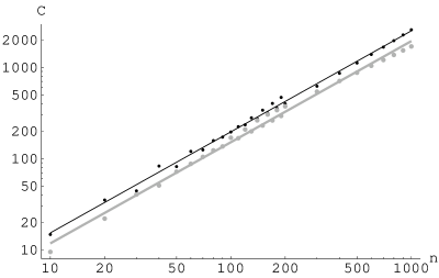
Figure 2: Expected search cost for maximum constrained 1-SAT vs. $n$ with the two phase choices: black and gray are Eq. (9) and Eq. (4.2.2), respectively. The lines are least squares fits to the points.

For Eq. (9), the number of steps giving the smallest cost grows very slowly, ranging from 2 to 4 over the range of variables shown in the figure. For Eq. (4.2.2), the largest probability for a solution is after $n/2+1$ steps. However, for the problems with $n\geq 200$, the small probability of a solution after just the first step is enough to give a slightly smaller search cost.

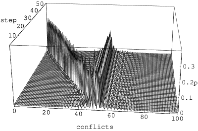
Figure 3: Evolution of the probability in assignments with different numbers of conflicts for the maximum constrained problem with $n=100$ using Eq. (4.2.2). The probability for a solution reaches about 0.3 after 51 steps, giving a search cost of about 170.

Further insight into the behavior of this algorithm is given by Fig. 3 which shows how the probability to have assignments with different numbers of conflicts varies with each step of Eq. (5). Specifically, for each step $j$ and each number of conflicts $c$, the figure shows the value of $\sum_{s}|\psi^{(j)}_{s}|^{2}$ where the sum is over all assignments $s$ with $c$ conflicts. As described in Appendix B.2, the amplitudes $\psi^{(j)}_{s}$ depend only on the number of conflicts in the assignment $s$. Thus each term in this sum is the same, giving ${n\choose c}|\psi^{(j)}_{c}|^{2}$ where $\psi^{(j)}_{c}$ denotes the amplitude of any of the assignments with $c$ conflicts. The initial condition (not shown) has equal probability, $2^{-n}$, in all assignments so the corresponding values in this plot would be ${n\choose c}2^{-n}$. We see a large probability in states with $n/2-(j-1)$ conflicts after step $j$, illustrating the effectiveness of Eq. (4.2.2) in using neighbor relations to move amplitude. Moreover, the large spike at 50 conflicts for step 1 shows the effectiveness of Eq. (10a) in concentrating amplitude in states with ${N_{\rm better}}={N_{\rm start}}$ for this problem. In this case, ${100\choose 50}|\psi^{(1)}_{50}|^{2}=0.39$ compared to its initial value ${100\choose 50}2^{-100}=0.08$.

The relatively low search costs and polynomial scaling are also observed for problems with somewhat fewer constraints than the maximum, e.g., $m=m_{\rm max}/2$, using this choice of phases. While this extends the range of good performance for the quantum algorithm, such a scaling also gives relatively easy problems for classical heuristics as well.

5.3 Problems with Fewer Constraints

The ability of this algorithm to concentrate amplitude into solutions for highly constrained problems is a significant improvement over unstructured search methods. However, such problems are inherently easy because they can be readily solved by classical heuristic methods, for both incremental and repair style searches. By contrast, the difficult search problems, on average, have an intermediate number of constraints [23]: not so few that most assignments are solutions, nor so many that any incorrect search choices can be quickly pruned. Specifically, for $k$-SAT the difficult problems have scaling $m=O(n)$, with the proportionality constant giving the largest concentration of hard cases depending on the choice of $k$. For instance, with $k=3$, the hard cases are concentrated near [10] $m=4.2n$. Thus it is important to examine the behavior of the algorithm for problems with fewer constraints. In this section we do so using the phase choice of Eq. (9).

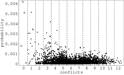
Figure 4: Probability in each assignment for a 3-SAT instance with $n=12$ after $J=5$ steps. The problem has $m=48$, with 4 solutions and $P_{\rm soln}=0.013$. The large gray points are the solutions.

A larger example of how the algorithm concentrates amplitude into solutions is shown in Fig. 4. It shows the values of $|\psi^{(J)}_{s}|^{2}$ for each of the $2^{n}$ assignments. The assignments are grouped by their number of conflicts and, within each group, by the integer corresponding to the binary representation of the assignment. For clarity, assignments with each number of conflicts are given the same amount of horizontal space in the plot, even though there are, e.g., many more assignments with 6 conflicts than with 0 or 12. There are $2^{12}$ assignments, so random selection would give a probability of about 0.0002 to each assignment. We see that the algorithm results in many states with relatively few conflicts, including the solutions, having considerably larger probabilities than due to random selection.

The figure also illustrates the variation in $|\psi^{(J)}_{s}|^{2}$ among the assignments showing that, unlike the extreme problem of the previous section, the amplitudes do not depend only on the number of conflicts. Rather the details of which constraints apply to each assignment give rise to the variation in values seen here. This variation precludes a simple theoretical analysis of the algorithm.

Figure 5: Expected search cost for random 3-SAT with at least one solution vs. $n$ with $m/n=4$ on a log plot. For each value of $n$, 1000 problem instances were used. Error bars showing the expected error in the estimate are included but are smaller than the size of the plotted points.

For problems near the transition from over- to underconstrained cases, the scaling behavior of this algorithm is shown in Fig. 5. Specifically, we generated random soluble instances of 3-SAT problems with $m=4n$, as described in §2. With $m=4n$, a large fraction of the randomly generated instances are soluble, so random soluble instances are readily generated. The nearly linear behavior on this log-plot indicates the seach cost grows exponentially for these problems. Thus this algorithm is not particularly effective for the hard problem instances, which are concentrated near the transition region of $m=4.2n$.

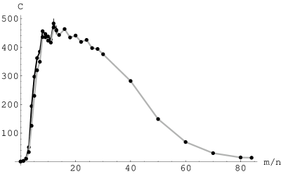
Figure 6: Expected search cost for random 3-SAT for $n=10$ vs. $m/n$. Each point represents 1000 problem instances, except only 100 random soluble instances are shown at $m/n$ equal to 12 and 13. The black line is for random soluble problems while the gray line is for problems with prespecified solution. Error bars showing the expected error in the estimate are included but, in most cases, are smaller than the size of the plotted points.

To show how this algorithm is capable of using structure to improve performance, we examined the behavior as a function of the number of constraints. To allow sampling the behavior of problems with many constraints we used random problems with prespecified solution to cover the full range of $m/n$, generated as described in §2. For comparison, we also examined the behavior of random soluble problems up to $m/n=15$. As shown in Fig. 6, the search cost eventually decreases as problems become highly constrained, though at a larger value of $m/n$ than for both the incremental quantum search method [22] and classical methods, whose cost is largest near the transition at $m=4.2n$. Thus the local quantum search method introduced here has only limited effectiveness at using structure to reduce search cost. Nevertheless, it is better than unstructured search for highly constrained problems.

6 Discussion

The algorithm presented here shows how the structure of search problems can be used as the basis of a quantum search algorithm. The algorithm is particularly effective for relatively highly constrained problems. It is less effective for problems with an intermediate number of constraints.

The algorithm might be improved in a number of ways. First, the initial motivation for the matrix $U$ was to maximally connect assignments to their neighbors. In fact, we found that the mapping allowed the algorithm to work best with fewer steps than might be expected from moving among neighbors one step at a time. It may be possible to design other mappings that do this even more effectively.

Another issue is the structure of the types of mappings possible with different choices of the phases for the diagonal matrix $D$. As we saw, the matrix elements depend only on the Hamming distance between the assignments when the diagonal elements of $D$ depend only on the number of 1-bits. It may be helpful to apply the testing operation, and consequent phase adjustments, more frequently as amplitude is moved to neighbors than is possible when $U$ has the largest possible mixing between neighbors. One such method is to decompose $U$ into a product of matrices, each of which introduces a smaller amount of mixing, e.g., using $U=WD^{1/s}W$, where $D^{1/s}$ is a diagonal matrix with $\tau_{h}=1$ if $h\leq n/2$ and $\tau=e^{i\pi/s}$ otherwise. Phase adjustments can then be introduced between the components of this product. Another method uses somewhat smaller values of $u_{1}$ while retaining real values for $U$ by picking a value $\alpha<n/2$ and using $\tau_{h}=1$ if $h\leq\alpha$ and $\tau=-1$ otherwise. The resulting mixing matrix has a more diffusive behavior, giving smaller changes with each step and hence more opportunity to apply the phase adjustment. Taken to an extreme, with $\alpha=0$, this recovers the diffusion matrix of the unstructured search [18], which moves too little amplitude among states at each step to finish rapidly.

There are also a variety of phase adjustment policies. Those studied here are effective for highly constrained problems, but we found that other choices can enhance performance in some cases. Furthermore, since we focus on typical or average behavior, other choices that do not improve the average but result in smaller variance would also be useful in improving the predictablility of the algorithm’s performance.

As a possible extension to this algorithm, it would be interesting to see whether the nonsolution sets with relatively high probability could be useful also. If so, the benefits of this algorithm would be greater than indicated by its direct ability to produce solution sets. This may also suggest similar algorithms for the related optimization problems where the task is to find the best solution according to some metric, not just one consistent with the problem constraints.

There remain a number of important questions. First, how are the results degraded by errors and decoherence, the major difficulties for the construction of quantum computers [27, 40, 19, 34]? While there has been recent progress in implementation [1, 8, 9, 17, 39], quantum approaches to error control [4, 37] and studies of decoherence in the context of factoring [7] it remains to be seen how these problems affect the algorithm presented here. However, two aspects of our algorithm may reduce the effect of errors. First, the algorithm is based on attempts to randomize phases of contributions to nonsolutions while maintaining similar phases for contributions to solutions. Since the precise values of the randomized phases are not critical, some additional variations due to noise should be tolerable. Second, for problems with $n$ variables the algorithm requires only $O(n)$ steps during which quantum coherence must be maintained. That is, coherence need not be maintained between successive trials of the algorithm. This contrasts with the $O(2^{n/2})$ coherent steps required by the unstructured algorithm [18]. Thus even though our algorithm may need to be repeated many times to give a good chance of finding a solution, it has less stringent coherence requirements which can simplify its hardware implementation.

The second remaining question is due to the algorithm’s restriction to CSPs with two values per variable. This contrasts with the method that constructs solutions incrementally [21] by operating in a greatly expanded search space. Other CSPs can be converted to equivalent problems with two values, but it is often better to operate directly with the problem as specified. Thus an important open question is whether the neighborhood-based mixing matrix can be effectively generalized to apply directly to CSPs with larger domain sizes.

Third, it would be useful to have a theory for asymptotic behavior of this algorithm for large $n$, even if only approximately in the spirit of mean-field theories of physics. This would give a better indication of the scaling behavior than the classical simulations, necessarily limited to small cases, and may also suggest better phase choices. Considering these questions may suggest simple modifications to the quantum map to improve its robustness and scaling.

Finally, there is the general issue of optimally using the information that can be readily extracted from search states. Local search methods rely on the number of conflicts and the neighborhood relations among states. In the method presented here, only a small amount of this information was actually used to determine the phase choices. Additional information is available on partial assignments, as used with incremental searches, but at the cost of involving a greatly expanded search space. Making fuller use of this available information could improve the performance, especially in conjunction with a theoretical understanding of the typical structure of classes of search problems [23].

Appendix A Appendix: Neighborhood Mixing Matrix

Here we show that the mixing matrix $U$ used in our algorithm is the unitary matrix depending only on the Hamming distance between states that gives the largest possible contribution to neighbors. We do this in two steps. We first show that matrices whose elements depend only on Hamming distance can be expressed in the form $WDW$ where $W$ is given by Eq. (7) and $D$ is diagonal with elements depending only on the number of 1-bits in the assignments. In the second step, we show that our choice of values for $D$ gives the largest possible mapping to neighbors among unitary matrices of this form.

A.1 Matrix Decomposition

For $n$ variables, the matrices have dimensions $2^{n}\times 2^{n}$ and elements determined by a set of values $u_{0},\ldots,u_{n}$, i.e., $U_{rs}=u_{d(r,s)}$. For example, with $n=2$ and the states binary order, i.e., 00, 01, 10, and 11, the matrix has the general form

$$U=\pmatrix{u_{0}&u_{1}&u_{1}&u_{2}\cr u_{1}&u_{0}&u_{2}&u_{1}\cr u_{1}&u_{2}&u_{0}&u_{1}\cr u_{2}&u_{1}&u_{1}&u_{0}\cr}$$ (11)

These matrices have a simple recursive decomposition when the states are in binary order, i.e., ordered by the value of the integer with corresponding binary representation, namely

$$U=\pmatrix{U_{0}&U_{1}\cr U_{1}&U_{0}\cr}$$ (12)

where the $2^{n-1}\times 2^{n-1}$ matrices $U_{0}$ and $U_{1}$ also have elements depending only on the Hamming distance between assignments, but considering only the first $n-1$ variables. An example of this decomposition can be seen in the structure of Eq. (11).

This decomposition gives a particularly simple expression for these matrices. Specifically, define the matrix $\hat{W}$ as

$$\hat{W}_{rs}=(-1)^{|r\wedge s|}$$ (13)

For example, when $n=2$,

$$\hat{W}=\pmatrix{1&1&1&1\cr 1&-1&1&-1\cr 1&1&-1&-1\cr 1&-1&-1&1\cr}$$ (14)

This matrix also has a recursive decomposition

$$\hat{W}=\pmatrix{\hat{W}^{\prime}&\hat{W}^{\prime}\cr\hat{W}^{\prime}&-\hat{W}^{\prime}\cr}$$ (15)

where $\hat{W}^{\prime}$ is the same matrix but defined on assignments to $n-1$ variables.

Now consider the product $\hat{W}U\hat{W}$. For $n=1$, this gives

$$\pmatrix{2(u_{0}+u_{1})&0\cr 0&2(u_{0}-u_{1})\cr}$$ (16)

which is a diagonal matrix. Now suppose that $\hat{W}U\hat{W}$ is always diagonal for any matrix with $U_{rs}$ depending only on $d(r,s)$ up to $n-1$ variables. Using the recursive decompositions of Eq. (12) and (15) then gives, for a matrix with $n$ variables

$$\hat{W}U\hat{W}=\pmatrix{2\hat{W}^{\prime}(U_{0}+U_{1})\hat{W}^{\prime}&0\cr 0&2\hat{W}^{\prime}(U_{0}-U_{1})\hat{W}^{\prime}\cr}$$ (17)

Each of the submatrices are diagonal because they involve products of the form $\hat{W}U\hat{W}$ for $n-1$ variables. Thus, by induction, $\hat{W}U\hat{W}$ is a diagonal matrix for all $n$, which we denote by $ND$, where $N=2^{n}$. Note that Eq. (7) is $W=\hat{W}/\sqrt{N}$. The matrix $W$ is symmetric and unitary [18]. In particular, $W$ is its own inverse: $WW=I$. Thus from $\hat{W}U\hat{W}=ND$ we obtain $U=WDW$.

Furthermore, the diagonal elements of $D$ depend only on the number of 1-bits in the assignments, i.e., $D_{rr}=\tau_{|r|}$ for some set of values $\tau_{0},\ldots,\tau_{n}$. To see this, we have

$$(\hat{W}U\hat{W})_{rr} = \sum_{xy}u_{d(x,y)}(-1)^{{|r\wedge x|}+{|y\wedge r|}}$$ (18)

$$= \sum_{d}u_{d}\sum_{z=0}^{{|r|}}(-1)^{z}{\sum_{xy}}^{\prime}1$$ (19)

where the innermost sum of the second line is over all assignments $x$ and $y$ for which $d(x,y)=d$ and ${|r\wedge x|}+{|y\wedge r|}=z$. For this inner sum, consider those assignments $x$ with exactly $\eta$ 1-bits in common with $r$, i.e., ${|r\wedge x|}=\eta$. There are ${{|r|}\choose\eta}2^{n-{|r|}}$ such choices for $x$. Then the $y$ sum counts the number of assignments $y$ such that $d(x,y)=d$ and ${|y\wedge r|}=z-\eta$. These assignments are characterized by $a$, the number of 1-bits they share with both $r$ and $x$. The number of such $y$ is readily seen to be

$${\eta\choose a}{{|r|}-\eta\choose z-\eta-a}{n-{|r|}\choose d-z+2a}$$

Summing over $a$ then gives the total number of assignments $y$, which we denote as $\nu(d,z,\eta,{|r|})$. Combining these observations gives

$$(\hat{W}U\hat{W})_{rr}=\sum_{d}u_{d}\sum_{z}(-1)^{z}\sum_{\eta}{{|r|}\choose\eta}2^{n-{|r|}}\nu(d,z,\eta,{|r|})$$ (20)

which depends only on the number of 1-bits in the assignment $r$.

In summary, any matrix whose values depend only on the Hamming distance between assignments can be written in the form $U=WDW$ where $D$ is a diagonal matrix with elements depending only on the number of 1-bits in the assignments. That is, the values for $u_{0},\ldots,u_{n}$ are uniquely determined by the diagonal values of $D$, which in turn are fully specified by the values $\tau_{0},\ldots,\tau_{n}$ for assignments with each possible number of 1-bits.

Since $W$ is unitary, $U$ will be unitary if and only if $D$ is. For diagonal matrices, the unitary condition is equivalent to the requirement that each diagonal element is a phase, i.e., a complex number whose magnitude equals one.

A.2 Maximum Mapping to Neighbors

To determine the choices for $\tau_{h}$ that give the largest possible value for $u_{1}$, we have

$$U_{rs}=\frac{1}{N}\sum_{h=0}^{n}\tau_{h}S_{h}(r,s)$$ (21)

where

$$S_{h}(r,s)=\sum_{t,{|t|}=h}(-1)^{{|r\wedge t|}+{|s\wedge t|}}$$ (22)

with the sum over all assignments $t$ with $h$ 1-bits.

A given 1-bit at position $e$ of $t$ contributes 0, 1 or 2 to ${|r\wedge t|}+{|s\wedge t|}$ when positions $e$ of $r$ and $s$ are both 0, have exactly a single 1-bit, or are both 1, respectively. Thus $(-1)^{{|r\wedge t|}+{|s\wedge t|}}$ equals $(-1)^{z}$ where $z$ is the number of 1-bits in $t$ that are in exactly one of $r$ and $s$. There are $({|r|}-{|r\wedge s|})+({|s|}-{|r\wedge s|})$ positions from which such bits of $t$ can be selected, and by Eq. (1) this is just $d(r,s)$. Thus the number of assignments $t$ with $h$ 1-bits and $z$ of these bits in exactly one of $r$ and $s$ is given by ${d\choose z}{n-d\choose h-z}$ where $d=d(r,s)$. Thus $S_{h}(r,s)=S_{hd}^{(n)}$ where

$$S_{hd}^{(n)}=\sum_{z}(-1)^{z}{d\choose z}{n-d\choose h-z}$$ (23)

so that $U_{rs}=u_{d(r,s)}$ with $u_{d}=\sum_{h}\tau_{h}S_{hd}^{(n)}/N$.

To select the values of $\tau_{h}$ that maximize $u_{1}$, note that $S_{01}^{(n)}=1$ and $S_{h1}^{(n)}={n-1\choose h}-{n-1\choose h-1}$. Thus $S_{h1}^{(n)}$ is positive for $n>2h$ and negative for $n<2h$, and $u_{1}$ is maximized by selecting $\tau_{h}$ to be 1 for $h<n/2$ and $-1$ for $h>n/2$. If $n$ is even, $S_{h1}^{(n)}$ is zero for $h=n/2$ so the choice of $\tau_{n/2}$ does not affect the value of $u_{1}$. In this case, we take $\tau_{n/2}=1$. These choices give $u_{1}=\frac{2}{N}{n-1\choose\lfloor n/2\rfloor}$ which scales as $\sqrt{2/(\pi n)}$ as $n\rightarrow\infty$. Note this is much larger than the off-diagonal matrix elements in the diffusion matrix used in the unstructured search algorithm [18], which are $O(1/N)=O(2^{-n})$.

This maximum neighbor mixing matrix is identical to that used with an incremental search method [22] but with a different interpretation of the search states. If instead we take $\tau_{0}=-1$ and the remaining values equal to one $U$ becomes the diffusion matrix of the unstructured search method [18].

Appendix B Appendix: Classical Simulation

A direct classical simulation of the quantum algorithm results in an exponential increase in the cost, limiting the empirical evaluation of the algorithm to small cases. Nevertheless, the simple structure of the mixing matrix $U$ can be used to reduce this cost penalty. It can be further reduced for the special case of soluble problems with the maximum possible number of constraints.

B.1 General Problems

As a practical matter, it is helpful if a quantum search method can be evaluated effectively on existing classical computers. Unfortunately, the exponential slowdown and growth in memory required for such a simulation severely limits the size of feasible problems. For example, Eq. (5) is a matrix multiplication of a vector of size $2^{n}$ so a direct evaluation requires $O(2^{2n})$ multiplications.

The cost of the classical simulation can be reduced substantially by exploiting the map’s simple structure. Specifically, the product $\hat{W}{\bf x}$ can be computed recursively using Eq. (15) giving

$$\hat{W}{\bf x}=\pmatrix{\hat{W}^{\prime}{\bf x^{(1)}}+\hat{W}^{\prime}{\bf x^{(2)}}\cr\hat{W}^{\prime}{\bf x^{(1)}}-\hat{W}^{\prime}{\bf x^{(2)}}\cr}$$ (24)

where $\bf x^{(1)}$ and $\bf x^{(2)}$ denote, respectively, the first and second halves of the vector $\bf x$. Thus the cost to compute $\hat{W}{\bf x}$ is $C(n)=2C(n-1)+O(2^{n})$ resulting in an overall cost of order $n2^{n}$ for this product as well as the full mapping step $U{\bf x}=(1/N)\hat{W}D\hat{W}{\bf x}$. While still exponential, this improves substantially on the cost for the direct evaluation on classical machines. An open question is whether other techniques could give approximate values for the behavior without an exponential cost on classical machines [6].

B.2 Maximally Constrained Problems

In general, the cost of a classical simulation of the quantum algorithm grows exponentially with the number of variables. However, the simulation cost is greatly reduced in some special cases where the amplitudes have a regular structure. One such case is provided by problems with the maximum possible number of constraints that still allows for a solution.

For such problems, the amplitudes depend only on the number of conflicts in each assignment, not their particular location. This observation allows for a smaller representation of the search state and hence an empirical study of larger cases. To see this, consider a 1-SAT problem with $n$ variables. The most constrained, but still soluble, case will have $n$ conflicts, each involving a distinct variable. Thus each variable has an associated “bad bit” value that causes a conflict. The number of conflicts in a given assignment $s$ is then just equal to the number of bad bits it contains. An assignment with $c$ conflicts will have $c$ neighbors with $c-1$ conflicts and $n-c$ neighbors with $c+1$ conflicts. Thus the neighborhood structure of the problem is uniquely determined by the number of conflicts in the assignments.

Suppose $\psi^{(j)}_{s}$ depends only on the number of conflicts in the assignment $s$. We need to show that after a single step, Eq. (5) gives values for $\psi^{(j+1)}_{r}$ that only depend on the number of conflicts in $r$. First note that the phase choice $\rho_{s}$ uses only the neighborhood structure of $s$, which for these problems depends only on the number of conflicts in $s$. Thus $\rho_{s}\psi^{(j)}_{s}$ depends only on $c$, the number of conflicts in $s$, and can be denoted by $\phi_{c}$. Since the mixing matrix $U_{rs}$ depends only on the Hamming distance between the assignments $r$ and $s$, Eq. (5) becomes

$$\psi^{(j+1)}_{r}=\sum_{d}u_{d}\sum_{c}\phi_{c}{\sum_{s}}^{\prime}1$$ (25)

where the inner sum is over assignments $s$ with $c$ conflicts and Hamming distance $d$ from the assignment $r$. Suppose $r$ has $b$ conflicts. Of the $c$ “bad bits” in $s$, $(c+b-d)/2$ are in common with those of $r$, and the remaining $(c-b+d)/2$ do not appear in $r$. The number of ways to construct such assignments $s$ is then

$${b\choose(c+b-d)/2}{n-b\choose(c-b+d)/2}$$

Thus the result of this mapping step depends only on the number of conflicts in the assignment $r$, preserving the simple structure of the search state. Thus we can represent the entire search state by simply keeping track of the amplitudes associated with each possible number of conflicts, i.e.,

$$\psi^{(j+1)}_{b}=\sum_{c}V^{\rm max}_{bc}\rho_{c}\psi^{(j)}_{c}$$ (26)

where $b$ and $c$ range from 0 to $n$ and

$$V^{\rm max}_{bc}=\sum_{d}u_{d}{b\choose(c+b-d)/2}{n-b\choose(c-b+d)/2}$$ (27)

Because the search state depends only on the number of conflicts and not their specific associated variables or values, we can, without loss of generality, choose the conflicts so that all the “bad bits” have the value 1, i.e., the unique solution of the problem has all variables equal to 0. With this choice, we can then make use of the decomposition of the mixing matrix. That is, $V^{\rm max}=W^{\rm max}D^{\rm max}W^{\rm max}$ where $D^{\rm max}$ is a diagonal matrix with $D^{\rm max}_{bb}$ equal to 1 for $b\leq n/2$ and $-1$ otherwise, and

$$W^{\rm max}_{bc}=\frac{1}{\sqrt{N}}\sum_{z}(-1)^{z}{b\choose z}{n-b\choose c-z}=\frac{S_{cb}^{(n)}}{\sqrt{N}}$$ (28)

from Eq. (23). Here the binomials in the sum count, for an assignment $r$ with $b$ 1-bits, the number of assignments $s$ with $c$ 1-bits that have ${|r\wedge s|}=z$. This decomposition is possible for this particular choice of the unique solution because the number of 1-bits correspond to the number of conflicts.

In this way, classical evaluation of Eq. (5) reduces to multiplication by matrices of size $(n+1)\times(n+1)$, with cost of order $n^{2}$.

Finally, 1-SAT problems with fewer than the maximum number of constraints also have the property that the amplitudes depend only on the number of conflicts in each assignment. So this compact representation could be used to study other cases of 1-SAT with many more variables than is feasible for a direct classical simulation.

References

- [1] Adriano Barenco, David Deutsch, and Artur Ekert. Conditional quantum dynamics and logic gates. Physical Review Letters, 74:4083–4086, 1995.
- [2] P. Benioff. Quantum mechanical hamiltonian models of Turing machines. J. Stat. Phys., 29:515–546, 1982.
- [3] Ethan Bernstein and Umesh Vazirani. Quantum complexity theory. In Proc. 25th ACM Symp. on Theory of Computation, pages 11–20, 1993.
- [4] Andre Berthiaume, David Deutsch, and Richard Jozsa. The stabilization of quantum computations. In Proc. of the Workshop on Physics and Computation (PhysComp94), pages 60–62, Los Alamitos, CA, 1994. IEEE Press.
- [5] Michel Boyer, Gilles Brassard, Peter Hoyer, and Alain Tapp. Tight bounds on quantum searching. In T. Toffoli et al., editors, Proc. of the Workshop on Physics and Computation (PhysComp96), pages 36–43, Cambridge, MA, 1996. New England Complex Systems Institute.
- [6] N. J. Cerf and S. E. Koonin. Monte Carlo simulation of quantum computation. In Proc. of IMACS Conf. on Monte Carlo Methods, 1997. Los Alamos preprint quant-ph/9703050.
- [7] I. L. Chuang, R. Laflamme, P. W. Shor, and W. H. Zurek. Quantum computers, factoring and decoherence. Science, 270:1633–1635, 1995.
- [8] J. I. Cirac and P. Zoller. Quantum computations with cold trapped ions. Physical Review Letters, 74:4091–4094, 1995.
- [9] David G. Cory, Amr F. Fahmy, and Timothy F. Havel. Nuclear magnetic resonance spectroscopy: An experimentally accessible paradigm for quantum computing. In T. Toffoli et al., editors, Proc. of the Workshop on Physics and Computation (PhysComp96), pages 87–91, Cambridge, MA, 1996. New England Complex Systems Institute.
- [10] James M. Crawford and Larry D. Auton. Experimental results on the crossover point in random 3SAT. Artificial Intelligence, 81:31–57, 1996.
- [11] D. Deutsch. Quantum theory, the Church-Turing principle and the universal quantum computer. Proc. R. Soc. London A, 400:97–117, 1985.
- [12] D. Deutsch. Quantum computational networks. Proc. R. Soc. Lond., A425:73–90, 1989.
- [13] David P. DiVincenzo. Quantum computation. Science, 270:255–261, 1995.
- [14] R. P. Feynman. Quantum mechanical computers. Foundations of Physics, 16:507–531, 1986.
- [15] Richard P. Feynman. QED: The Strange Theory of Light and Matter. Princeton Univ. Press, NJ, 1985.
- [16] M. R. Garey and D. S. Johnson. Computers and Intractability: A Guide to the Theory of NP-Completeness. W. H. Freeman, San Francisco, 1979.
- [17] Neil Gershenfeld, Isaac Chuang, and Seth Lloyd. Bulk quantum computation. In T. Toffoli et al., editors, Proc. of the Workshop on Physics and Computation (PhysComp96), page 134, Cambridge, MA, 1996. New England Complex Systems Institute.
- [18] Lov K. Grover. A fast quantum mechanical algorithm for database search. In Proc. of the 28th Annual Symposium on the Theory of Computing (STOC96), pages 212–219, 1996.
- [19] Serge Haroche and Jean-Michel Raimond. Quantum computing: Dream or nightmare? Physics Today, pages 51–52, August 1996.
- [20] Tad Hogg. Statistical mechanics of combinatorial search. In Proc. of the Workshop on Physics and Computation (PhysComp94), pages 196–202, Los Alamitos, CA, 1994. IEEE Press.
- [21] Tad Hogg. Quantum computing and phase transitions in combinatorial search. J. of Artificial Intelligence Research, 4:91–128, 1996. Available online at http://www.jair.org/abstracts/hogg96a.html.
- [22] Tad Hogg. A framework for structured quantum search. 1997. Available at xxx.lanl.gov/abs/quant-ph/9701013.
- [23] Tad Hogg, Bernardo A. Huberman, and Colin Williams. Phase transitions and the search problem. Artificial Intelligence, 81:1–15, 1996.
- [24] Peter Hoyer. Efficient quantum transforms. Los Alamos preprint http://xxx.lanl.gov/abs/quant-ph/9702028, February 1997.
- [25] S. Kirkpatrick, C. D. Gelatt, and M. P. Vecchi. Optimization by simulated annealing. Science, 220:671–680, 1983.
- [26] Scott Kirkpatrick and Bart Selman. Critical behavior in the satisfiability of random boolean expressions. Science, 264:1297–1301, 1994.
- [27] Rolf Landauer. Is quantum mechanically coherent computation useful? In D. H. Feng and B-L. Hu, editors, Proc. of the Drexel-4 Symposium on Quantum Nonintegrability. International Press, 1994.
- [28] Seth Lloyd. A potentially realizable quantum computer. Science, 261:1569–1571, 1993.
- [29] Michael Luby and Wolfgang Ertel. Optimal parallelization of Las Vegas algorithms. Technical report, Intl. Comp. Sci. Inst., Berkeley, CA, July 14 1993.
- [30] Alan Mackworth. Constraint satisfaction. In S. Shapiro, editor, Encyclopedia of Artificial Intelligence, pages 285–293. Wiley, 1992.
- [31] N. David Mermin. Is the moon there when nobody looks? Reality and the quantum theory. Physics Today, pages 38–47, April 1985.
- [32] Steven Minton, Mark D. Johnston, Andrew B. Philips, and Philip Laird. Minimizing conflicts: A heuristic repair method for constraint satisfaction and scheduling problems. Artificial Intelligence, 58:161–205, 1992.
- [33] Remi Monasson and Riccardo Zecchina. The entropy of the k-satisfiability problem. Phys. Rev. Lett., 76:3881–3885, 1996.
- [34] Christopher Monroe and David Wineland. Future of quantum computing proves to be debatable. Physics Today, pages 107–108, November 1996.
- [35] A. Nijenhuis and H. S. Wilf. Combinatorial Algorithms for Computers and Calculators. Academic Press, New York, 2nd edition, 1978.
- [36] Bart Selman, Hector Levesque, and David Mitchell. A new method for solving hard satisfiability problems. In Proc. of the 10th Natl. Conf. on Artificial Intelligence (AAAI92), pages 440–446, Menlo Park, CA, 1992. AAAI Press.
- [37] P. Shor. Scheme for reducing decoherence in quantum computer memory. Physical Review A, 52:2493–2496, 1995.
- [38] Peter W. Shor. Algorithms for quantum computation: Discrete logarithms and factoring. In S. Goldwasser, editor, Proc. of the 35th Symposium on Foundations of Computer Science, pages 124–134. IEEE Press, November 1994.
- [39] Tycho Sleator and Harald Weinfurter. Realizable universal quantum logic gates. Physical Review Letters, 74:4087–4090, 1995.
- [40] W. G. Unruh. Maintaining coherence in quantum computers. Physical Review A, 51:992–997, 1995.