Experimental Quantum Error Correction

Abstract

Quantum error correction is required to compensate for the fragility of the state of a quantum computer. We report the first experimental implementations of quantum error correction and confirm the expected state stabilization. In NMR computing, however, a net improvement in the signal-to-noise would require very high polarization. The experiment implemented the 3-bit code for phase errors in liquid state state NMR.

PACS numbers: 03.65.Bz, 89.70.+c,89.80.th,02.70.–c

Quantum computers exploit the superposition principle to solve some problems much more efficiently than any known algorithm for their classical counterparts. These problems include factoring large numbers[1] (thereby breaking public key cryptography), combinatorial searching[2] and simulations of quantum systems[3, 4, 5]. Exploiting the power of quantum computation was thought to be physically impossible due to the extreme fragility of quantum information[6, 7]. This judgment was demonstrated to be overly pessimistic when quantum error-correction techniques[8, 9, 10] were found to protect quantum information against corruption due to imperfect control and decoherence. It is now known that for physically reasonable models of decoherence a quantum computation can be as long as desired with arbitrarily accurate answers, provided the error rate is below a threshold value[11, 12, 13, 14]. Thus decoherence and imprecision are no longer considered insurmountable obstacles to realizing a quantum computer.

The chief remaining obstacle to quantum computing is the difficulty of finding suitable physical systems whose quantum states can be accurately controlled. Devices based on ion traps [15] have so far been limited to two bits[16]. Recently, liquid state NMR techniques have been shown to be capable of quantum computations with at least three bits [17, 18]. This makes it possible, for the first time, to experimentally implement the simplest quantum error-correcting codes, and so test these ideas in physical systems with a variety of decoherence, dephasing and relaxation phenomena.

In room temperature liquid state NMR, one can coherently manipulate the internal states of the coupled spin $1\over 2$ nuclei in each of an ensemble of molecules subject to a large external magnetic field. Although the ensemble nature of the system and the small energy of each spin imply that the set of accessible states is highly mixed, it has been shown that experimental methods exist that can be used to isolate the pure state behavior of the system, thus permitting limited application of NMR to quantum computation[19, 20].

Here we describe the implementation of a quantum error-correcting code which compensates for small phase errors due to fluctuations in the local magnetic field. The behavior of this code was measured for two systems: The ¹³C labeled carbons in alanine subject to the correlated phase errors induced by diffusion in a pulsed magnetic field gradient, and the proton and two labeled carbons in trichloroethylene (TCE) subject to its natural relaxation processes. In alanine, we observed correction of first-order errors for a given input state, while in TCE we demonstrated state preservation of an arbitrary state by error correction.

In NMR loss of phase coherence may be both due to bona fide irreversible decoherence[21] and due to dephasing which can be reversed by spin echo. Both lead to symptoms which, in an ensemble, are identical from the standpoint of quantum computation. Both can be corrected using the same scheme we shall demonstrate below.

It is important to comment on the applicability of this technique to ensemble quantum computing. Although our experiments validate the usefulness of error correction for quantum computing with pure states, there is a substantial loss of signal associated with the use of ancilla spins in weakly polarized systems. We argue that in this setting, the loss of signal involved in exploiting ancillas removes any advantage for computation gained by error correction, at least unless the system is sufficiently polarized to enable the generation of nearly pure states. Nevertheless, our experiments demonstrate that error-correcting codes can be implemented, and that they behave as predicted.

The simple three-bit quantum error-correcting code used here is designed to compensate to first order for small random phase fluctuations. These fluctuations constitute a random evolution of the state

$$|b_{1}b_{2}b_{3}\rangle ~{}\longrightarrow~{} e^{-i(\theta_{1}\mbox{\boldmath$\scriptstyle\sigma$}_{\rm z}^{1}+\theta_{2}\mbox{\boldmath$\scriptstyle\sigma$}_{\rm z}^{2}+\theta_{3}\mbox{\boldmath$\scriptstyle\sigma$}_{\rm z}^{3})}|b_{1}b_{2}b_{3}\rangle$$ (2)

$$=~{}e^{i((-1)^{b_{1}}\theta_{1}+(-1)^{b_{2}}\theta_{2}+(-1)^{b_{3}}\theta_{3})}|b_{1}b_{2}b_{3}\rangle~{},$$

where $b_{i}$ is $0$ or $1$, $\theta_{i}$ is a random phase variable, and $\mbox{\boldmath$\sigma$}_{z}^{i}$ is the Pauli matrix acting on the $i$’th spin. The $\theta_{i}$ depend on the error rates in the model, which is described in detail below.

The error-correcting code itself is a phase variant of the classical three bit majority code with a decoding technique that preserves the quantum information in the encoded state. Let $|+\rangle=(|0\rangle+|1\rangle)/\sqrt{2}$ and $|-\rangle=(|0\rangle-|1\rangle)/\sqrt{2}$. The state $(\alpha|000\rangle+\beta|100\rangle)$ is encoded as $\alpha|+\,+\,+\rangle+\beta|-\,-\,-\rangle$ by a unitary transformation. The first-order expansion of the operator in Eq. (2) in the small random phases is

$${\bf 1}-i\theta_{1}\mbox{\boldmath$\sigma$}_{z}^{1}-i\theta_{2}\mbox{\boldmath$\sigma$}_{z}^{2}-i\theta_{3}\mbox{\boldmath$\sigma$}_{z}^{3}~{},$$ (3)

which evolves the encoded state to

$$\alpha|++\,+\rangle+\beta|--\,-\rangle \rightarrow ~{}~{}\alpha|++\,+\rangle+\beta|--\,-\rangle$$ (7)

$$-i\theta_{1}(\alpha|-+\,+\rangle+\beta|+-\,-\rangle)$$

$$-i\theta_{2}(\alpha|+-\,+\rangle+\beta|-+\,-\rangle)$$

$$-i\theta_{3}(\alpha|++\,-\rangle+\beta|--\,+\rangle)~{}.$$

The different errors map the encoded state into orthogonal subspaces. Thus one can determine which error occurred without destroying the encoded quantum information. This is accomplished by a measurement which reveals the subspace the state has moved into. After decoding, the original state of the first spin can then be restored by a unitary transformation, while the other two spins contain information (the syndrome) about the error which occurred. A network which accomplishes the encoding, decoding and error-correction steps is shown in Figure 1.

In NMR experiments, non-unitary processes are classified as spin-lattice and spin-spin relaxation [22, 23]. The former involves an exchange of energy with the non-spin degrees of freedom (the lattice), and returns the spins to thermal equilibrium. The latter leads to a loss of phase coherence. For spin $\frac{1}{2}$ nuclei, both processes are due to fluctuating local magnetic fields. The three spin code corrects for errors due to locally fluctuating fields along the z axis.

We focus on a weakly coupled three-spin system where the strongest contribution to coherence loss is from external fields which contribute the Hamiltonian

$${\cal H}_{\rm R}~{}\equiv~{}\gamma^{1}{\bf I}^{1}\cdot{\bf B}^{1}(t)+\gamma^{2}{\bf I}^{2}\cdot{\bf B}^{2}(t)+\gamma^{2}{\bf I}^{3}\cdot{\bf B}^{3}(t)~{},$$ (8)

where ${\bf I}=({\bf I}_{\rm x},{\bf I}_{\rm y},{\bf I}_{\rm z})$ and ${\bf I}_{u}={1\over 2}\mbox{\boldmath$\sigma$}_{u}$ ($u={\rm x,y,z}$). In the case of slowly varying external fields the induced random phase fluctuations are identical to those described in Eq. (2). As a result, the off-diagonal elements of the density matrix decay exponentially at a rate which depends on the fields ${\bf B}^{k}$ at each spin, their gyromagnetic ratios $\gamma^{k}$, the coherence order and the zero frequency components of the spectral densities of the fields. The “coherence order” is the difference between the total angular momenta along the z-axis of the two states $|b\rangle$, $|b^{\prime}\rangle$ (in units of $\hbar/2$)[24].

To obtain a clean demonstration of error correction, a simple error model was implemented precisely in the case of alanine. This implementation used the random molecular motion induced by diffusion in a constant field gradient to mimic the effect of a slowly varying random field. This is achieved by turning on an external field gradient $\nabla_{\rm z}{\bf B}=\partial B_{\rm z}/\partial z$ across the sample for a time $\delta$. This modifies the magnetization in the sample with a phase varying linearly along the z direction according to $\partial\phi/\partial z=n\delta\gamma\partial B_{\rm z}/\partial z$, where $n$ is the coherence order of the density matrix element and $\gamma$ is the gyromagnetic ratio. A reverse gradient is used to refocus the magnetization after allowing molecular diffusion to take place for amount of time $t$. As a result of random spin displacement $\Delta z$, the phases of the spins are not returned to their original values but are randomly modified by $(n\delta\gamma\partial B_{\rm z}/\partial z)\Delta z$. For a gaussian displacement profile with a width of $\sqrt{2Dt}$, the effective decoherence time of this process is proportional to the diffusion constant $D$ as well as to the square of the coherence order $n$ [24]:

$$\frac{1}{\tau}~{}=~{}\left(\frac{\partial\phi}{\partial z}\right)^{2}D~{}=~{}\gamma^{2}(\nabla_{\rm z}{\bf B})^{2}n^{2}\delta^{2}D~{}.$$ (9)

This artificially induced “decoherence” in the alanine experiments is an example of completely correlated phase scrambling. This occurs naturally if all the spins have equal gyromagnetic ratios in the slow motion regime. We used TCE to demonstrate error-correction in the presence of the natural decoherence and dephasing of a molecule where $T_{2}\ll T_{1}$.

Most NMR experiments are described using the product operator formalism [25]. This formalism describes the state as a sum of products of the operators ${\bf I}_{x}^{k}$, ${\bf I}_{y}^{k}$, ${\bf I}_{z}^{k}$. The identity component of such a sum is the same for any state and is usually suppressed to yield the “deviation” (traceless) density matrix. The effect of error-correction can be understood from the point of view of this formalism. As an example, consider encoding the state ${\bf I}_{\rm z}^{1}$ using two ancillas initially in their ground states. Up to a constant factor, the initial state is described by

$$\mbox{\boldmath$\rho$}_{\sf A} = {\bf I}_{\rm z}^{1}(\mbox{$\frac{1}{2}$}{\bf 1}+{\bf I}_{\rm z}^{2})(\mbox{$\frac{1}{2}$}{\bf 1}+{\bf I}_{\rm z}^{3})$$ (10)

$$= \mbox{$\frac{1}{4}$}{\bf I}_{\rm z}^{1}+\mbox{$\frac{1}{2}$}{\bf I}_{\rm z}^{1}{\bf I}_{\rm z}^{2}+\mbox{$\frac{1}{2}$}{\bf I}_{\rm z}^{1}{\bf I}_{\rm z}^{3}+{\bf I}_{\rm z}^{1}{\bf I}^{2}{\bf I}_{\rm z}^{3}~{}.$$ (11)

The density matrix $\mbox{\boldmath$\rho$}_{\sf A}$ consists of an incoherent sum of four terms.

After encoding the state is

$$\mbox{\boldmath$\rho$}_{\mathsf{B}}~{}\equiv~{}\mbox{$\frac{1}{4}$}\left({\bf I}_{\mathrm{x}}^{1}+{\bf I}_{\mathrm{x}}^{2}+{\bf I}_{\mathrm{x}}^{3}+4\,{\bf I}_{\mathrm{x}}^{1}{\bf I}_{\mathrm{x}}^{2}{\bf I}_{\mathrm{x}}^{3}\right)~{}.$$ (12)

In the case of completely correlated phase errors, this decays as

$$\mbox{\boldmath$\rho$}_{\sf C} ~{}\equiv~{} \mbox{$\frac{1}{4}$}\left(\left({\bf I}_{\rm x}^{1}+{\bf I}_{\rm x}^{2}+{\bf I}_{\rm x}^{3}\right)e^{-t/\tau}\right.$$ (15)

$$\left.\mbox{}\hskip 3.5pt+\left(3{\bf I}_{\rm x}^{1}{\bf I}_{\rm x}^{2}{\bf I}_{\rm x}^{3}+{\bf I}_{\rm x}^{1}{\bf I}_{\rm y}^{2}{\bf I}_{\rm y}^{3}+{\bf I}_{\rm y}^{1}{\bf I}_{\rm x}^{2}{\bf I}_{\rm y}^{3}+{\bf I}_{\rm y}^{1}{\bf I}_{\rm y}^{2}{\bf I}_{\rm x}^{3}\right)e^{-t/\tau}\right.$$

$$\left.\mbox{}\hskip 3.5pt+\left({\bf I}_{\rm x}^{1}{\bf I}_{\rm x}^{2}{\bf I}_{\rm x}^{3}-{\bf I}_{\rm x}^{1}{\bf I}_{\rm y}^{2}{\bf I}_{\rm y}^{3}-{\bf I}_{\rm y}^{1}{\bf I}_{\rm x}^{2}{\bf I}_{\rm y}^{3}-{\bf I}_{\rm y}^{1}{\bf I}_{\rm y}^{2}{\bf I}_{\rm x}^{3}\right)e^{-9t/\tau}\right)~{}.$$

Decoding and error correction mixes these states together so as to cancel the initial decay of the first spin. The reduced density matrix for the first spin becomes

$$\mbox{\boldmath$\rho$}_{\sf E}^{1}~{}\equiv~{}\mbox{$\frac{1}{8}$}{\bf I}_{\mathrm{z}}^{1}(9e^{-t/\tau}-e^{-9t/\tau})~{}\approx~{}{\bf I}_{\mathrm{z}}^{1}(1-{9\over 2}t^{2}/\tau^{2}+\cdots)~{}.$$ (16)

The effect of error correction can be seen from the absence of terms depending linearly on $t$. Similar results can be obtained for other initial states and also for uncorrelated phase errors.

In the alanine experiments, each of the four product operators in the sum of Eq. 11 was realized in a separate experiment, and the final state after encoding and decoding inferred by adding the results. The loss of polarization over time in each product operator was measured explicitly in each experiment. The results were added computationally to simulate the effect of the Toffoli gate and are shown in Figure 2. The components of ${\bf I}_{\mathrm{z}}^{1}{\bf I}_{\mathrm{z}}^{2}{\bf I}_{\mathrm{z}}^{3}$ which evolved as a single and a triple coherence when encoded were separated by gradient labeling [24]. The initial slopes of the decay curves for each operator were estimated by linear square fit to the logarithm of the measured intensities. The values obtained are $-0.0034$ ( ${\bf I}_{\mathrm{z}}^{1}$), $-0.0030$ ($2{\bf I}_{\mathrm{z}}^{1}{\bf I}_{\mathrm{z}}^{2}$), $-0.0047$ ($2{\bf I}_{\mathrm{z}}^{1}{\bf I}_{\mathrm{z}}^{3}$), $-0.0038$ ($4{\bf I}_{\mathrm{z}}^{1}{\bf I}_{\mathrm{z}}^{2}{\bf I}_{\mathrm{z}}^{3}$, single coherence) and $-0.0395$ ($4{\bf I}_{\mathrm{z}}^{1}{\bf I}_{\mathrm{z}}^{2}{\bf I}_{\mathrm{z}}^{3}$, triple coherence) When the slopes are added as required for error-correction with a pseudopure input, we get a measured net slope of $0.00081$, which should be compared to the slopes for the single coherences whose average is $-0.0037$. The net curve has quadratic behavior for small delays to within experimental error.

The goal of our experiments with TCE was to establish the behavior of encoding/decoding and error correction on all possible initial states subject to the natural decoherence and dephasing. The spins were prepared in the states

$$\rho({1\over 2}{\bf 1}+{\bf I}_{z}^{2})({1\over 2}{\bf 1}+{\bf I}_{z}^{3}),$$ (17)

with $\rho$ one of the four inputs ${1\over 2}{\bf 1}$, ${\bf I}_{z}^{1}$, ${\bf I}_{x}^{1}$, ${\bf I}_{y}^{1}$. Any possible input is just a linear combination of these four states. We used gradient methods to directly generate the four states of Eq. 17 with a series of experiments. They were then subjected to pulse sequences for encoding and decoding (experiment I) with a variable delay between the two operations. Decoherence and dephasing take place during the delay. The reduced density matrix on the first spin (the output) was measured. In the second experiment (II) decoding was followed by error correction before the output was determined. Ideally the output would be identical to the input. The measured outputs were compared to the ideal ones by computing the “entanglement fidelity” [26]. This is a useful measure of how well the quantum information in the input is preserved. Entanglement fidelity is the sum of the correct polarization left in the output state for each input. More precisely, given input ${\bf I}_{a}^{1}$, let $f_{a}$ be the relative polarization of ${\bf I}_{a}^{1}$ in the output compared to the input. Then $f={1\over 4}(1+f_{x}+f_{y}+f_{z})$, this formula is correct for processes which do not affect the completely mixed state ${1\over 2}{\bf 1}$. The results for nine different delays are shown in Figure 3. The curves show that error correction decreases the initial slope by a factor of $\sim 10$ (by square fit to the logarithm).

Our demonstration of error-correction does not imply that error-correction can be used to overcome the problems of high temperature ensemble quantum computing. In this model of quantum computing, the initial state can be described as a small, linear deviation from the infinite temperature equilibrium. Thus, the deviation is proportional to a Hamiltonian of $n$ weakly interacting particles. In this limit no method of error-correction based on externally applied, time dependent fields can improve the polarization of any particle by more than a factor proportional to $\sqrt{n}$ [27]. If one wishes to use error-correction an even bigger problem is encountered: The initial state of the ancillas used for each encoding/decoding cycle must be pure. In the high temperature regime, the best we can do to ensure that is to generate a pseudopure deviation in the ancillas. Unfortunately, this deviation has to be created simultaneously on all ancillas, leading to an exponential reduction in polarization proportional to the total number of ancillas required [28]. This always exceeds the loss of polarization. Another problem is the inability to reuse ancilla bits. This has two consequences. The first is that decoherence rapidly removes information in the state, leading to computations which are logarithmically bounded in time [29]. Second, the total number of ancillas required is proportional to the time-space product of the computation, rather than to a power of it’s logarithm.

Our work shows that liquid state NMR can be used to test fundamental ideas in quantum computing and communication involving non-trivial numbers of bits subject to a variety of errors. Our experiments demonstrate for the first time the state preserving effect of the three bit phase error-correcting code. The first-order behavior was established to high accuracy for a specific state in alanine, while the overall effect was observed and the improvement in state recovery verified in TCE. These experiments confirm not only the validity of theories of quantum error correction in a simple case, but also demonstrate the ability, in liquid state NMR, to control the state of three spin-half particles. This is an important advance for quantum computing, as this is the first system where this degree of control has been successfully implemented.

Acknowledgments

We thank Jeff Gore for his help with the simulations. This work was supported by, or in part by, the U. S. Army Research Office under contract/grant number DAAG 55-97-1-0342 from the DARPA Ultrascale Computing Program. E. K., R. L. and W. H. Z thank the National Security Agency for support.

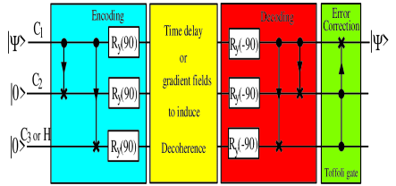
FIG. 1.: Network for encoding, decoding and error correction. The circuit describes the evolution of the 3 bits as a function of time. The gate $\bullet$—$>$–x corresponds to a control-not, i.e a gate which flips the target bit (x) if the control bit ($\bullet$) is in the state $|1\rangle$. $R_{y}(90)$ represent a single bit gate corresponding to a rotation by an angle of $\pi/2$ around the $y$-axis. The Tofolli gate flips the target bit (x) if the two control bits ($\bullet$) are in the state $|1\rangle$. A detailed implementation of these gates is given in [17]. The information carrying bit is carbon 1 (see Figures 2 and 3) in both experiments.

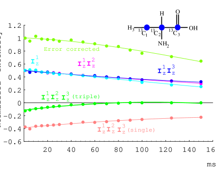
FIG. 2.: The intensities of the magnetization of the first spin after applying the dephasing and decoding procedures described in the text, together with single exponential fits to the intensities versus the dephasing time $\tau$. The three mixed states ${\bf I}_{\rm z}^{1}$, ${\bf I}_{\rm z}^{1}{\bf I}_{\rm z}^{2}$, ${\bf I}_{\rm z}^{1}{\bf I}_{\rm z}^{3}$, evolved as single quantum coherences during $\tau$, whereas ${\bf I}_{\mathrm{z}}^{1}{\bf I}_{\mathrm{z}}^{2}{\bf I}_{\mathrm{z}}^{3}$ evolved as a mixture of single and triple quantum coherences, which have been plotted separately (single and triple). The sum of these intensities and the corresponding fits (Error corrected) give the intensities and fit characteristics of the same experiment using a pseudopure state (see text). The initial slope of the total is close to zero, thus showing that the error-correction procedure was able to cancel loss of coherence of the pseudopure state to first order.

FIG. 3.: Experimentally determined entanglement fidelities for the TCE experiments after decoding (red) and after decoding and error correction (green). The continuous curves are interpolations of the data points. The broken curves were determined by simulating the pulse sequence using the measured coupling constants and estimated $T_{2}$’s of $1.1s$ (C1), $0.6s$ (C2) and $3s$ (H). Differences between experimental and theoretical curves are attributed to lack of precise knowledge of the error model. Errors in the data points are approximately $0.05$. Note that since the proton $T_{2}$ is much longer than that of the carbons, the long term gain in fidelity is partially due to recovery of polarization from the proton. The demonstration of error correction lies in the initial slope. The curves show that error correction decreases the initial slope by a factor of $\sim 10$ (by square fit to the logarithm).

REFERENCES

- [1] P. W. Shor. In Proceedings of the 35’th Annual Symposium on Foundations of Computer Science, pages 124–134, Los Alamitos, California, 1994. IEEE Press.
- [2] L. K. Grover. quant-ph/9605043.
- [3] R. P. Feynman. Found. of Phys., 16:507–531, 1986.
- [4] S. Lloyd. Science, 273:1073–1078, 1996.
- [5] C. Zalka. Proc. Roy. Soc. of London A, in press.
- [6] R. Landauer. Phil. Trans. Roy. Soc. of London, 353:367–376, 1995.
- [7] W. G. Unruh. Phys. Rev. A, 51:992–997, 1995.
- [8] P. W. Shor. Phys. Rev. A, 52:2493–, 1995.
- [9] A. Steane. Proc. Roy. Soc. of London A, 452:2551–, 1996.
- [10] P. W. Shor. In Proceedings of the Symposium on the Foundations of Computer Science, pages 56–65, Los Alamitos, California, 1996. IEEE press. quant-ph/9605011.
- [11] E. Knill, R. Laflamme, and W. Zurek. Science, vol 279, p.342, 1998.
- [12] D. Aharonov and M. Ben-Or. quant-ph/9611025, to appear in STOC’97, 1996.
- [13] J. Preskill. Proc. Roy. Soc. of London A, in press.
- [14] A. Yu. Kitaev. preprint, 1996.
- [15] J. Cirac and P. Zoller. Phys. Rev. Let., 74:4091–, 1995.
- [16] C. Monroe, D. M. Meekhof, B. E. King, W. M. Itano, and D. J. Wineland. Phys. Rev. Lett., 75:4714–, 1995.
- [17] D. G. Cory, M. P. Price, and T. F. Havel. Physica D, 1998. In press (quant-ph/9709001).
- [18] R. Laflamme, E. Knill, W.H. Zurek, P. Catasti and S. Marathan. quant-ph/9709025, 1997.
- [19] D. G. Cory, A. F. Fahmy, and T. F. Havel. Proc. Nat. Acad. of Sciences of the U. S., 94:1634–1639, 1997.
- [20] N. A. Gershenfeld and I. L. Chuang. Science, 275:350–356, 1997.
- [21] W. H. Zurek Physics Today, October, 1991.
- [22] A. Abragam. Principles of Nuclear Magnetism. Clarendon Press, Oxford, U.K., 1961.
- [23] R. R. Ernst, G. Bodenhausen, and A. Wokaun. Principles of Nuclear Magnetic Resonance in One and Two Dimensions. Clarendon Press, Oxford, U.K., 1987.
- [24] C. P. Slichter. Principles of Magnetic Resonance (3rd ed.). Springer Verlag, 1990.
- [25] O. W. Sörensen, G. W. Eich, M. H. Levitt, G. Bodenhausen, and R. R. Ernst. Prog. NMR Spect., 16:163–, 1983.
- [26] B. Schumacher. Phys. Rev. A 54, 2614-2628, 1996.
- [27] O. W. Sörensen. Prog. NMR Spect., 21:503–569, 1989.
- [28] W. S. Warren. Science, 277:1688–1698, 1997.
- [29] D. Aharonov and M. Ben-Or. quant-ph/9611028, 1996.