Noise, errors and information in quantum amplification

Abstract

We analyze and compare the characterization of a quantum device in terms of noise, transmitted bit-error-rate (BER) and mutual information, showing how the noise description is meaningful only for Gaussian channels. After reviewing the description of a quantum communication channel, we study the insertion of an amplifier. We focus attention on the case of direct detection, where the linear amplifier has a 3 decibels noise figure, which is usually considered an unsurpassable limit, referred to as the standard quantum limit (SQL). Both noise and BER could be reduced using an ideal amplifier, which is feasible in principle. However, just a reduction of noise beyond the SQL does not generally correspond to an improvement of the BER or of the mutual information. This is the case of a laser amplifier, where saturation can greatly reduce the noise figure, although there is no corresponding improvement of the BER. Such mechanism is illustrated on the basis of Monte Carlo simulations.

1 Introduction

In order to exploit the bandwidth available in the optical domain the evolution of optical communications urges conversion of hybrid electro-optical devices towards all-optical ones. For long distance communications the losses along the optical fiber decrease the transmitted power and introduce communication errors, thus being the crucial limitation to the development of this kind of technology. On the other hand, an amplifier along the line restores the power level, but introduces noise of quantum origin. For direct detection, which would allow to achieve the ultimate channel capacity [1], an optical phase insensitive amplifier used in the linear regime introduces 3 decibels of noise. Such noise has long been considered as an unsurpassable limit [2] — the so called “standard quantum limit” (SQL)— which, however is just a peculiarity of the linear phase insensitive amplifier (PIA) [3].

In order to recover the transparency of an optical network one needs to achieve a perfect amplification that, by itself, does not introduce any additional disturbance. Indeed, as suggested by Yuen [4], it is possible in principle to achieve such ideal amplification also for direct detection, although there is still no actual device that can attain it in practice. With this aim one could try to improve the performance of an existing amplifier by driving it far from the linear regime, and going beyond the SQL. In Ref. [3] it has been shown that this is indeed possible for a saturable laser amplifier, where in an intermediate-saturating regime one can accomplish noise suppression with still sizeable gains. The objective of Ref. [3] was originally to prove that the SQL can be actually breached in a concrete case. In a following debate [5, 6] it has been pointed out that the noise is not the significant quantity for evaluating the goodness of an amplifier, and one should better resort to the original problem of the transmitted bit-error-rate (BER). However, Ref. [5] still considered the PIA as the reference standard quantum amplifier, whereas, as clarified in Ref. [6], the ideal photon number amplifier (PNA) of Yuen indeed could greatly improve the transmitted BER of the PIA.

In this paper we reconsider the problem of characterizing the quality of a low-noise amplifier from the beginning. We clarify that the quantity that unambiguously determines the behavior of a device inserted in a communication channel is the so called “mutual information” between the input and the output. For a binary channel, the BER is essentially equivalent to the mutual information for small error probabilities, whereas it remains an ambiguous characterization for any pathological situation. On the other hand, we will also show that the characterization in terms of noise is still meaningful for Gaussian communications channels.

As the noise characterization [3] is not sufficient to establish whether a saturable amplifier can perform better than a linear one, here we present a careful analysis of a laser amplifier in a quantum regime, and compare it with an ideal PIA. We illustrate the mechanism that underlies a noise reduction under saturation, and explain why such reduction does not correspond to any improvement of the BER. We will show that this is typical of the saturation mechanism, whereas, in general, a noise reduction may correspond to an improvement of the BER, and, indeed, for an ideal PNA such an improvement can be actually achieved.

The outline of the paper is the following. In Sec. 2 we give a brief introduction to the basic concepts of information theory that are needed for a complete characterization of the operation of a quantum amplifier. Such concepts are then specialized to the case of a quantum communication channel in Sec. 3, where a complete description of the transmission of quantum signals and the characterization of a quantum amplifier are given. In Sec. 4 the linear Gaussian channel is discussed. This channel is of particular interest because it is the only case where a quantum amplifier can be equivalently characterized in terms of mutual information and in terms of noise. In view of the subsequent comparison between the performances of a linear and a saturable amplifier, in Sec. 5 the conventional linear PIA is reviewed and the SQL is derived. In Sec. 6 the laser saturable amplifier is presented and analyzed on the basis of the Fokker-Planck equation derived by Haake and Lewenstein [7]. In Sec. 7, after presenting some numerical tests of the theory and of the Monte Carlo simulation method, we compare the performance of the saturable amplifier to the one of the linear PIA. The conclusions are then given in Sec. 8.

2 Basic concepts of information theory

A communication channel between a transmitter and a receiver can be viewed as composed of three basic constituents: an encoder, a transmission line, and a decoder. The encoder transforms the input of the channel —i.e. the message to be transmitted— into a proper set of physical signals that are impinged into the transmission line. In this schematic representation the transmission line includes all possible physical processes that affect the signal that carries the message from the sender to the receiver, including all noise sources and any kind of device (e.g. amplifiers) inserted along the line. The decoder applies a set of operations on the received signal, like measurements and data processing of the results, and then gives the reconstructed message at the output of the channel. If no transformation modifies the signals along the line, then the encoded message can be perfectly reconstructed, otherwise errors can arise at the decoder, and the intrinsic potential of the channel decreases.

The significant quantity that measures the efficiency of a communication channel is the mutual information. Let us define it first in the case of a classical discrete channel, and then generalize it later to the continuous and quantum cases.

By definition, a discrete channel transmits only symbols belonging to a numerable set. Suppose that the input of the channel is a symbol from the set (or alphabet) $\{x_{j},j=1,...,J\}$ of $J$ elements with a priori probabilities $\{p_{j},j=1,...,J\}$ ($\sum_{i=1}^{J}p_{i}=1$), whereas the output is a symbol from the set $\{y_{k},k=1,...,K\}$ of $K$ elements (the two sets need not be equal). The two sets are linked by specifying the conditional probabilities $Q_{k|j}$ that the output is $y_{k}$ given the symbol $x_{j}$ at the input. The mutual information is given by

$$I(X;Y)=\sum_{j=1}^{J}\sum_{k=1}^{K}p_{j}Q_{k|j}\log_{2}\frac{Q_{k|j}}{\sum_{i}p_{i}Q_{k|i}}$$ (1)

and quantifies the degree of knowledge (in bits) that the output random variable $Y$ gives about the input random variable $X$ (by the capital letter $X\equiv\{x_{j},p_{j},j=1,\cdots,J\}$ we denote the random variable, namely the set of symbols $\{x_{i}\}$ along with the corresponding probability distribution $\{p_{i}\}$). The mutual information can also be written as follows

$$I(X;Y)=H(X)-H(X|Y)\;,$$ (2)

namely as the difference between the entropy at the input

$$H(X)=-\sum_{j=1}^{J}p_{j}\log_{2}p_{j}$$ (3)

and the conditional entropy at the output

$$H(X|Y)=-\sum_{k=1}^{K}q_{k}\sum_{j=1}^{J}P_{j|k}\log_{2}P_{j|k}\;,$$ (4)

where $q_{k}=\sum_{i}p_{i}Q_{k|i}$ is the unconditioned probability of the output symbol $y_{k}$ and $P_{j|k}=p_{j}Q_{k|j}/q_{k}$ is the conditioned probability that symbol $x_{j}$ was transmitted given that symbol $y_{k}$ is received. In the limiting case $X\equiv Y$ that input and output alphabets coincide and the channel is noiseless ($Q_{j|k}=\delta_{jk}$), one has

$$I(X;X)=H(X)\;,$$ (5)

namely the information transmitted through a noiseless channel is just the entropy of the input alphabet. In the opposite limiting case that the input and output random variables are completely uncorrelated ($Q_{j|k}=q_{j}$ for all $k$) the mutual information vanishes.

The definition of mutual information (1) can be straightforwardly generalized to the case of a continuous set of symbols $x\in{\cal X}$ and $y\in{\cal Y}$, with a priori probability density $p(x)$ and conditional probability density $Q(y|x)$. Here the sums in (1) replaced by integrals as follows

$$I(X;Y)=\int_{\cal X}dx\int_{\cal Y}dy\ p(x)Q(y|x)\log_{2}\frac{Q(y|x)}{\int dz\ p(z)Q(y|z)}\;.$$ (6)

Let us now consider the case of a binary channel, where two different symbols “0” and “1” (which make one “bit”) are transmitted with equal a priori probabilities $p_{0}=p_{1}=1/2$. Usually a binary channel is characterized by the probability of making errors at the decoder, called “bit error rate” (BER), and defined as follows

$$B=\frac{1}{2}\Bigl{(}Q_{0|1}+Q_{1|0}\Bigr{)}\;.$$ (7)

In Eq. (7) $Q_{1|0}$ is named “false alarm probability” (the probability of detecting “1” when the signal “0” was transmitted), whereas $Q_{1|1}=1-Q_{0|1}$ is called “detection probability”. Among the possible choices of sets of independent probabilities, in the following we adopt the couple $\{Q_{0|1},Q_{1|0}\}$, in terms of which all quantities of interest (e.g. BER $B$ and mutual information $I$) can be expressed. The mutual information of the binary channel takes the form

$$I = \frac{1}{2}\Biggl{[}(1-Q_{1|0})\log_{2}\frac{2(1-Q_{1|0})}{1-Q_{1|0}+Q_{0|1}}+Q_{0|1}\log_{2}\frac{2Q_{0|1}}{1-Q_{1|0}+Q_{0|1}}+$$ (8)

$$+ Q_{1|0}\log_{2}\frac{2Q_{1|0}}{1-Q_{0|1}+Q_{1|0}}+(1-Q_{0|1})\log_{2}\frac{2(1-Q_{0|1})}{1-Q_{0|1}+Q_{1|0}}\Biggr{]}\;.$$ (9)

In the binary channel the BER gives the same characterization as the mutual information in the limiting case of small error probabilities ($Q_{1|0},Q_{0|1}\ll 1$). Here, $I$ can be expanded at first order in $Q_{1|0}$ and $Q_{0|1}$, and one has

$$B\ll 1\Rightarrow I\cong 1-B\;.$$ (10)

Notice, however, that the BER and the mutual information generally do not give the same description of the channel, as one can have channels with the same BER but having different mutual information, and vice versa. For instance, consider the case $B=0$ corresponding to $Q_{0|1}=Q_{1|0}=0$ (namely no errors are made in the identification of the binary symbol at the output). As mentioned before this means that the information is maximum, i.e. $I(X;Y)=1$. On the other hand, for $B=1$ one has $Q_{0|1}=Q_{1|0}=1$, namely the output symbol is always interpreted in the wrong way: in this case, however, the mutual information is still unit, and, in fact, it is possible to reconstruct the transmitted message without ambiguity by swapping the symbols “0” and “1” at the output. Moreover, one can have different values of the mutual information that correspond to the same BER, just by varying the probabilities of error and keeping their sum fixed.

As shown in the above examples, the mutual information gives a more complete description of the communication channel than the BER, and hence it should be adopted as the right quantity to characterize the channel. In the rest of this paper, however, we will use the BER, because in our case the probabilities of error are so small that BER is equivalent to the mutual information via Eq. (10).

3 The quantum communication channel

In this section we specialize the above concepts to the quantum communication channel, where the information is encoded on quantum states. In the first two subsections we give a characterization of the channel in terms of mutual information, and in terms of gain and noise figure of the devices inserted along the line. Finally, in Subsec. 3.3 we review the description of the dynamical evolution of the quantum state along the transmission line, with the insertion of both amplification and losses.

3.1 Mutual information in the quantum channel

In a quantum channel the symbols to be transmitted are encoded into density operators $\rho_{x}$ on the Hilbert space ${\cal H}$ of the dynamical system that supports the communication. The alphabet (which can be either discrete or continuous) is distributed according to an a priori probability density $p(x)$, which also determines the mixture $\bar{\rho}$ given by

$$\bar{\rho}=\int dx\ p(x)\rho_{x}\;.$$ (11)

The set of states $\rho_{x}$ and the probability density $p(x)$ are globally referred to as ”encoding”. The transmission line includes all dynamical transformations of the encoded states between the encoder and the decoder. In the Schrödinger picture these are described by a completely positive (CP) map $\rho\to\rho_{t}=E_{t}(\rho)$ acting on the density matrix $\rho$ that carries the information through the channel. The last step in the communication channel is the decoding operation, where the recognition of the transmitted symbol is established as the result of a quantum measurement. In the general case this is conveniently described by means of a probability operator measure[8, 9] (POM), which extends the notion of orthogonal-projector-valued measure associated to customary quantum observables. The POM $d\Pi(y)$ provides the probability distribution $p[\rho](y)\;dy$ of the random outcome $y$ of the measurement according to the rule

$$p[\rho](y)\;dy=\hbox{Tr}[\rho\;d\Pi(y)]\;.$$ (12)

In order to have a genuine probability $dP[\rho](y)$, a POM must satisfy the positivity condition

$$d\Pi(y)\geq 0$$ (13)

as a consequence of the positivity of the density operator $\rho$. Normalization of the probability $p(y)$ is guaranteed by the completeness relation

$$\int d\Pi(y)=1\;.$$ (14)

Each measurement apparatus is described by a POM. Actually, the POM comes from a customary orthogonal projection-valued measure that includes also the degrees of freedom of the apparatus, which are partially traced out in order to give a description of the system alone. Notice that the correspondence between measuring apparatus and POM’s is not one-to-one, since different detectors can be described by the same POM. In a quantum communication channel the POM specifies the conditional probabilities in the mutual information (6), namely

$$Q(y|x)\;dy=\hbox{Tr}[E_{t}(\rho_{x})\;d\Pi(y)]\;.$$ (15)

The value of the mutual information depends on all the three steps of the communication channel: encoding, transmission and decoding. The maximum of $I(X,Y)$ over all possible a priori probability densities $p(x)$ for a given constraint (typically the average power along the line) and for an ideal channel (namely $E_{t}=1$ is the identical transformation) is called “capacity” $C$ of the channel, whereas the global maximum obtained optimizing also over both encoding and decoding is called “ultimate quantum capacity”. For fixed average power $\bar{n}$, using the Holevo-Ozawa-Yuen information bound[1, 10] it can be proved that the ultimate quantum capacity for a quantum–optical channel is achieved by direct detection and number-state encoding, with $\bar{\rho}$ being the thermal state with photon number $\bar{n}$.

3.2 Gain and noise in amplification

Let us now consider the effects of the insertion of an amplifier in a transmission line. The performances of a quantum amplifier are described in terms of the gain and the disturbance caused by the device to the transmitted signal. As already discussed, the best quantity to characterize the disturbance is the loss of mutual information with respect to the case of ideal transmission. However, although the noise figure is significant only for Gaussian channels (see Sec. 4), this is the quantity that is customarily used to characterize the disturbance of the amplifier.

Both gain and noise figure generally depend on the overall configuration of the channel, i.e. on the particular encoded states and on the kind of detection at the decoder. The gain is defined as the ratio between the output and the input signals as follows

$$G={{{S}_{out}}\over{{S}_{in}}}\;,$$ (16)

where the signals $S_{in,out}$ are defined as the difference between expectation values

$$S_{in,out}=\mbox{Tr}\{O\ \rho_{in,out}\}-\mbox{Tr}\{O\ \upsilon_{in,out}\},$$ (17)

where $\rho_{out}=E_{t}(\rho_{in})$, $\upsilon_{out}=E_{t}(\upsilon_{in})$, $E_{t}$ is the CP map of the amplifier from the input to the output, $O$ is the detected operator and $\upsilon$ is a reference state. For optical amplifiers at the input of the channel the state $\upsilon_{in}$ is usually the vacuum, but it is generally transformed into a non-vacuum state $\upsilon_{out}$ as it evolves through the amplifier. An amplifier is called ”linear” when the gain does not depend on the input state $\rho_{in}$. Notice that, as the signal depends on the detection scheme defined by the observable $O$, in principle the linear character of a device depends on the kind of detection at the output.

The noise figure quantifies the degradation of the signal-to-noise ratio (SNR) from the input to the output, and is defined as

$$R=SNR_{in}/SNR_{out}\;.$$ (18)

In Eq. (18) the signal-to-noise ratio is given by

$$SNR={S}^{2}/{N}\;,$$ (19)

where $N$ is the quantum noise $\langle\Delta O^{2}\rangle_{\rho}=\hbox{Tr}(\rho O^{2})-[\hbox{Tr}(\rho O)]^{2}$ for detected observable $O$ averaged over the alphabet with a priori probability distribution $p(x)$, i.e.

$$N=\int dx\ p(x)\langle\Delta O^{2}_{x}\rangle_{\rho_{x}}\;.$$ (20)

Notice that the definitions of both signal $S$ and noise $N$ can be easily generalized to the case of a detector described by a non orthogonal POM $d\Pi$, just replacing the ensemble averages by

$$\langle y^{k}\rangle_{p}=\mbox{Tr}\left[\rho\int d\Pi(y)\ y^{k}\right]\;.$$ (21)

When characterizing the quality of an amplifier, usually one resorts to determining the noise added by the amplifier along the line. However, a quantitative characterization should be based on the change of mutual information due to the amplifier insertion. For this reason, we define as “ideal” an amplifier that does not degrade an optimized channel, namely that leaves the information invariant in a channel where the information has been already maximized over all possible encodings and decodings for a given constraint. As a rescaling of the probability distribution $Q(y|x)\to Q(G^{-1}y|x)$ leaves the mutual information in Eq. (6) invariant, an amplifier that rescales the probability by the gain $G$ —hence maps the observable $O$ to $GO$— is ideal (the pathological situation of bounded spectrum is not considered, as in this case the concept itself of amplification is meaningless). For such an ideal amplifier one has unit noise figure $R=1$, independently of the input state. It is clear that for a non optimized channel, an amplifier can increase the mutual information, and, actually, this is its purpose. In fact, by rescaling the detection spectrum the amplifier expands the effective dimension of the Hilbert space that supports the relevant part of the transmitted information. The loss of information in a non optimized channel can be caused either by an irreversible dynamics along the line (this is the case of the loss), and/or by a mismatch between coding and detection, or by low quantum efficiency of the detector. In the first case it is clear that the amplifier must be inserted before the leak of information, namely as a preamplifier, whereas in the second case it can be inserted just before the detector, the quantum efficiency representing essentially an irreversible evolution inside the detector. Notice that the configuration of the channel with the amplifier before the loss may violate the physical constraint of limited power, and hence the best configuration is a distributed gain along the line.

In the case of a binary channel, with symbols “0” and “1” corresponding to the input states $\rho_{0}\equiv\upsilon$ and $\rho$ ($\upsilon$ being the vacuum), the gain is given by Eq. (16), and Eq. (20) rewrites

$${N}={1\over 2}\left(\langle\Delta O^{2}\rangle_{\rho_{0}}+\langle\Delta O^{2}\rangle_{\rho}\right)\;.$$ (22)

In Sec. 4 we will show the equivalence between BER and noise figure in the characterization of a Gaussian binary channel, and in Subsec. 7.2 the difference between the two quantities will be revealed in the cases of linear and saturable amplifiers. The characterization of an amplifier given in this section is also suited to describe an attenuator (i.e. a “deamplifier”) or the loss itself, where now $G<1$, whereas, generally, for an amplifier one strictly has $G>1$.

3.3 CP maps, master equation and Fokker - Planck equation.

In this subsection we will briefly introduce the quantum treatment of the evolution equations for a signal state through a transmission line in the presence of losses or active devices (e.g. amplifiers). Both losses and amplifiers are treated as open systems [12]. In an amplifier the mode of radiation that undergoes amplification—the ”signal” mode—resonantly interacts with other modes of radiation (parametric amplifier) or with matter degrees of freedom (active medium amplifier). The necessary energy for amplification is provided by “pump” modes, whereas “idler” modes guarantee resonance conditions and phase-matching. All modes different from the signal mode (i.e. the “system”) act globally as a reservoir, and the signal mode undergoes a non unitary irreversible transformation (the only exception is the ideal phase sensitive amplifier, where the transformation is unitary). On the other hand, in the presence of a loss (a beam splitter or a lossy cavity/fiber) the signal mode is gradually lost into external modes. The dynamical evolution of the density matrix $\rho$ of an open system is obtained by partially tracing over all the external degrees of freedom (globally referred to as the “probe”) and is described by a map of the form

$$\rho_{t}=E_{t}(\rho)=\mbox{Tr}_{P}\left[U_{t}\,\rho_{P}\otimes\rho\,U_{t}^{\dagger}\right]\;,$$ (23)

where $U_{t}$ is a unitary operator and $\rho_{P}$ is the density matrix for the probe. By expanding the trace over a (numerable) orthonormal set, Eq. (23) rewrites as follows

$$E_{t}(\rho)=\sum_{k}V_{k}\rho V_{k}^{\dagger}\;,\qquad\sum_{k}V_{k}^{\dagger}V_{k}=1\;,$$ (24)

which is the Stinespring representation[12] of a normal trace-preserving CP-map. The infinitesimal version of Eq. (23) or (24) is usually referred to as the “master equation”. Lindblad proved that the most general form of a valid master equation is given by[13]

$$\partial_{t}\rho_{t}=\sum_{k}{\cal D}[A_{k}]\rho_{t}\;,\qquad{\cal D}[A]\rho\doteq A\rho A^{\dagger}-\frac{1}{2}\left\{A^{\dagger}A,\rho\right\}\;,$$ (25)

where $\{\,,\,\}$ denotes the anticommutator, $A_{k}$ are generic complex operators, and ${\cal D}[A]$ are called Lindblad super-operators (a “superoperator” is a map that acts on operators both on the left and on the right sides).

The master equation can be transformed into a differential equation for an ordinary unknown c-number function (instead of an operator $\rho$) using the Wigner representation of the density matrix. When the order of derivatives can be truncated at the second one, the equation has the form of a Fokker Planck equation (FPE)

$$\partial_{t}W_{s}(\alpha,{{\alpha}^{*}};t)=\left[\partial_{\alpha}\alpha\ Q_{s}(\alpha,{{\alpha}^{*}})+\partial_{{\alpha}^{*}}{{\alpha}^{*}}Q^{*}_{s}(\alpha,{{\alpha}^{*}})+\frac{1}{2}\vec{\vec{\nabla}}_{\alpha}:{\vec{\vec{D}}}_{s}(\alpha,{{\alpha}^{*}})\right]W_{s}(\alpha,{{\alpha}^{*}};t)\;,$$ (26)

where $(Q_{s},Q_{s}^{*})$ is the drift vector, ${\vec{\vec{D}}}_{s}$ the diffusion matrix, $\vec{\vec{\nabla}}_{\alpha}$ is the matrix of second derivatives

$$\vec{\vec{\nabla}}_{\alpha}=\left(\matrix{\partial^{2}_{\alpha{{\alpha}^{*}}}&\partial^{2}_{\alpha\alpha}\cr\partial^{2}_{{{\alpha}^{*}}{{\alpha}^{*}}}&\partial^{2}_{{{\alpha}^{*}}\alpha}}\right)\ ,$$ (27)

and $W_{s}(\alpha,{{\alpha}^{*}})$ is the generalized Wigner function of the radiation mode with annihilation operator $a$, defined as follows

$$W_{s}(\alpha,\alpha^{*})\doteq\int{{d^{2}\lambda}\over{\pi}}\ X_{s}(\lambda,\lambda^{*})\exp\left(\alpha\lambda^{*}-\alpha^{*}\lambda\right)\;.$$ (28)

The Wigner function $W_{s}(\alpha,\alpha^{*})$ is the Fourier transform of the generating function of the $s$-ordered moments

$$X_{s}(\lambda,\lambda^{*})=\hbox{Tr}\left[\rho\exp\left(\lambda a^{{\dagger}}-\lambda^{*}a\right)\right]\exp\left({1\over 2}s|\lambda|^{2}\right)\;,$$ (29)

with the moments given by

$$\hbox{Tr}\left[\rho\left\{a^{{\dagger}n}a^{m}\right\}_{s}\right]={{\partial^{n}}\over{\partial\lambda^{n}}}\left.{{\partial^{m}}\over{\partial(-\lambda^{*})^{m}}}\right|_{\lambda=0}X_{s}(\lambda,\lambda^{*})=\int{{d^{2}\alpha}\over\pi}\ W_{s}(\alpha,\alpha^{*})\alpha^{*n}\alpha^{m}\;.$$ (30)

In the following sections we will only consider the case $s=0$, which corresponds to symmetrical ordering. Here we notice that the functions $W_{s}(\alpha,\alpha^{*})$ are not generally probability distributions, as they are not positive definite, and for this reason they are named “quasi–probabilities”. Only for $s\leq-1$ one has $W_{s}(\alpha,\alpha^{*})\geq 0$ for all $\alpha$. In particular for $s=-1$, which corresponds to antinormal ordering, $W_{s}(\alpha,\alpha^{*})$ is the probability distribution of the ideal measurement of the complex field (heterodyne detection), whereas for $s<-1$ it represents the same measurement with quantum efficiency $\eta_{het}={2}/({1-s})<1$.

From the Wigner generalized function one can obtain the homodyne detection probability distribution in form of the marginal integration

$$P_{s}(x)=\int{{dy}\over{\pi}}W_{s}(x+iy,x-iy)\;,$$ (31)

and now the quantum efficiency $\eta_{hom}$ of the homodyne detector is related to the ordering parameters by $\eta_{hom}={1}/{(1-s)}$.

In the rest of the present section we will consider a FPE with constant drift and diffusion coefficients of the form

$$\partial_{t}W_{s}(\alpha,{{\alpha}^{*}})=\left[Q(\partial_{\alpha}\alpha+\partial_{\alpha^{*}}{{\alpha}^{*}})+2D_{s}\partial^{2}_{\alpha{{\alpha}^{*}}}\right]W_{s}(\alpha,{{\alpha}^{*}}).$$ (32)

Eq. (32) can be solved analytically, with solution in form of the following Gaussian convolution

$$W_{s}(\alpha,{{\alpha}^{*}};t)=\frac{1}{\pi\Delta_{s}^{2}(t)}\int d^{2}\beta\ \exp\left[-\frac{|\alpha-\beta e^{-Qt}|^{2}}{\Delta_{s}^{2}(t)}\right]W_{s}(\beta,\beta^{*};0)\;\!,$$ (33)

where

$$\Delta_{s}^{2}(t)=\frac{D_{s}}{Q}(1-e^{-2Qt})\;.$$ (34)

For homodyne detection the marginal integration of the FPE leads to the Ornstein-Uhlenbeck equation (OUE)

$$\partial_{t}P_{s}(x;t)=\left[Q\partial_{x}x+\frac{1}{2}D_{s}\partial^{2}_{xx}\right]P_{s}(x;t)\;,$$ (35)

again with solution in form of the Gaussian convolution

$$P_{s}(x;t)=\frac{1}{\sqrt{2\pi d_{s}^{2}(t)}}\int dx^{\prime}\ \exp\left[-\frac{(x-x^{\prime}e^{-Qt})^{2}}{2d_{s}^{2}(t)}\right]P_{s}(x^{\prime};0)\!\;,$$ (36)

where

$$d_{s}^{2}(t)=\frac{D_{s}}{2Q}(1-e^{-2Qt})\;.$$ (37)

Notice that the diffusion terms in (32) and (35) generally depend on the efficiency of the detection apparatus. It is straightforward to see from Eqs.(33) and (36) that the gain for the corresponding variable (the field amplitude for Eq. (32) and the quadrature for Eq. (35)) is given by $G=e^{-Qt}$, and does not depend on the input state. Therefore, the processes described by Eqs. (32) and (35) correspond to the case of linear amplification for $Q<0$, or to the case of linear loss for $Q>0$. When the diffusion coefficient in Eqs. (32) and (35) vanishes, the evolution of the corresponding probability distribution is just given by the rescaling of the field variable $\alpha$, namely

$$W_{s}(\alpha,{{\alpha}^{*}};t)=\frac{1}{G^{2}}W_{s}(G^{-1}\alpha,G^{-1}{{\alpha}^{*}};0)\;\!$$ (38)

and, for the OUE, for the homodyne variable $x$

$$P_{s}(x;t)=\frac{1}{G}P_{s}(G^{-1}x;0)\!\;.$$ (39)

In this case, for perfect detection (described either by $W_{-1}$ or by $P_{0}$) the device is ideal. For detection with $\eta<1$, one can even have $D_{s}<0$ [11], which means that the ideal amplifier can improve the SNR and the mutual information. For heterodyne detection ($W_{-1}$), the ideal amplifier is the so called phase insensitive amplifier (PIA), which will be described in detail in Sec. 5. For homodyne detection ($P_{0}$) the ideal amplifier is the phase sensitive amplifier (PSA), which is described by a Ornstein Uhlenbeck equation of the form (35) with vanishing diffusion term. For direct detection, namely detection of the photon number of the radiation field, the ideal amplifier is called “photon number amplifier” (PNA) [4]. In the following section, we will consider these linear devices inserted in a linear Gaussian channel with Gaussian input probability.

4 The linear Gaussian channel

A linear Gaussian channel is a particular type of channel where the evolution equation is given by Eq. (26) or Eq. (35), i.e. it has a Gaussian Green function, and the encoded states at the input are themselves described by Gaussian probability distributions. The time–evolved probability distributions are easily obtained from Eqs. (33) and (36) as follows

$$W_{s}(\alpha,{{\alpha}^{*}};t)=\frac{1}{\pi\Delta_{s}^{2}(t)}\exp\left[-\frac{|\alpha-\alpha_{0}e^{-Qt}|^{2}}{\Delta_{s}^{2}(t)}\right]\;\!,\qquad$$ (40)

$$\Delta_{s}^{2}(t)=\frac{D_{s}}{Q}(1-e^{-2Qt})+\Delta_{s}^{2}(0)e^{-2Qt}\;,$$ (41)

and

$$P_{s}(x;t)=\frac{1}{\sqrt{2\pi d_{s}^{2}(t)}}\exp\left[-\frac{(x-x_{0}e^{-Qt})^{2}}{2d_{s}^{2}(t)}\right]\!\;,\qquad d_{s}^{2}(t)=\frac{D_{s}}{2Q}(1-e^{-2Qt})+d_{s}^{2}(0)e^{-2Qt}\;.$$ (42)

For a Gaussian channel, the probability distribution remains Gaussian at all times, and the evolution is completely characterized by the changes of mean value and variance, whereas the drift and diffusion coefficients are constant. In this simple case the mutual information and the noise figure can be easily computed for different configurations [11].

For the Gaussian channel, we now analyze the relations between the three different criteria: information, noise, and BER.

Relation between noise and information

If we consider a continuous alphabet described by Gaussian states with variance $\Delta^{2}$, and transmitted according to an a priori Gaussian probability distribution with variance $\delta^{2}$, the mutual information takes the form

$$I=\frac{1}{2}\log_{2}\left(1+\frac{\delta^{2}}{\Delta^{2}}\right).$$ (43)

Hence the mutual information is just a function of the noise $N=\Delta^{2}$ and of the variance $\delta^{2}$ of the a priori probability distribution.

Relation between noise and BER

The use of the BER actually pertains to the case of a binary channel. For a Gaussian channel, the two states “0” and “1” have Gaussian probability distributions at the output centered around two different values. The two Gaussians are overlapping, and one discriminates between “0” and “1” upon introducing a threshold $\vartheta$, such that one has “0” signal for $y<\vartheta$ and “1” for $y>\vartheta$. For output described by probability densities $q_{0}$ and $q_{1}$, the error probabilities $Q_{0|1}$ and $Q_{1|0}$ are given by

$$Q_{0|1} = \int_{x\leq\vartheta}dy\ q_{1}(y)$$ (44)

$$Q_{1|0} = \int_{x\geq\vartheta}dy\ q_{0}(y)\;,$$ (45)

The BER obviously depends on the threshold $\vartheta$, which must be optimized in order to obtain the minimum value. For Gaussian functions this corresponds to putting $\vartheta$ at the crossing point between the graphs of the two output distribution probabilities, and the BER is just the overlap area. When the input states have the same variance, the optimal threshold $\vartheta=S/2$ is placed exactly in the middle between the mean values of the two distributions. From Eq. (44) one has

$$B=1-\Phi\left(\root \of{\frac{SNR}{8}}\right)\simeq\root \of{\frac{8}{\pi\ SNR}}\ \ e^{-\frac{1}{8}SNR},$$ (46)

where the symbol $\simeq$ stands for asymptotic value for large SNR. As the error function $\Phi$ is monotone, one can see that for binary Gaussian channels the SNR and the BER criteria are essentially the same.

For non Gaussian channels, the equivalence between the three different criteria is generally not valid. In fact, we cannot establish a general rule for the time evolution of the shapes of the probability distributions. Therefore, there may occur cases where the noise figure is small because there is little broadening of the probability, but the BER is high because the broadening is not symmetrical around the mean value and the overlap region increases more than the area below the external tails of the distributions. As we will see in Sec. 6, this is the case of a saturable amplifier. In principle, there might be also opposite situations, where the noise figure gets worse because of a broadening of the probabilities, but at the same time the BER improves because the broadening is dominant in the non overlapping region of the two probabilities. For non Gaussian channels, therefore, the characterization of a device performance in terms of noise figure may be significantly different from the one based on the BER analysis, and the latter must then be considered instead.

5 The phase insensitive amplifier

A phase insensitive linear amplifier is described by the following master equation

$$\partial_{t}\rho_{t}=2\left[A{\cal D}[a^{{\dagger}}]+B{\cal D}[a]\right]\rho_{t}\;,$$ (47)

where the superoperator $\cal D$ is defined in Eq. (25) and $A>B$. As a consequence of the invariance ${\cal D}[ae^{-i\phi}]={\cal D}[a]$, the device is phase insensitive, namely it amplifies the field independently of the value of its phase. The case $B>A$ describes a linear attenuation process. With $A$ and $B$ proportional to the atomic populations of the upper and lower lasing levels respectively, Eq. (47) describes an active medium amplifier in the linear regime (i.e. far from saturation). On the other hand, for $A={{\Gamma}\over 2}\bar{m}$ and $B={{\Gamma}\over 2}(\bar{m}+1)$ the same equation describes a field mode with photon lifetime $\Gamma^{-1}$ damped towards the thermal distribution with $\bar{m}$ average photons.

Eq. (47) has the following general CP-map solution[14]

$$\rho_{t}=\mbox{Tr}_{P}[U_{t}\,\rho\otimes\nu\,U_{t}^{{\dagger}}]\;,\qquad U_{t}=\left\{\begin{array}[]{ll}\exp[-\arctan\sqrt{e^{\Gamma t}-1}(ab^{\dagger}-a^{\dagger}b)]&(B>A)\;,\\ \exp[-\hbox{arctanh}\sqrt{1-e^{-\Gamma t}}(a^{\dagger}b^{\dagger}-ab)]&(A>B)\;,\end{array}\right.$$ (50)

where $\Gamma/2=|A-B|$, and the second field mode $b$ is an additional mode, called “idler”, that is initially in the thermal state $\nu$ with average photons $\bar{m}=\mbox{min}\{A,B\}/|A-B|$ [$A$ and $B$ must be non negative, otherwise one would have negative idler photons]. The idler mode $b$ is needed for the unitarity requirement of the quantum evolution of the fields [21]. Ideal amplification is achieved when the idler mode $b$ is initially in the vacuum state. In the case of finite temperature, when the mode $b$ is initially in the thermal state with a non vanishing number of photons $\bar{m}$, the amplifier is not ideal ($B\neq 0$).

Let us now study the performance of the PIA for different kinds of detection. Corresponding to the master equation (47) one can obtain a Fokker-Planck equation of the form (26) with $Q=B-A$ and $2D_{s}=A+B+s(A-B)$. For ideal heterodyne detection ($s=-1$) the device is ideal for $B=0$ (ideal phase insensitive amplifier), because the diffusion coefficient vanishes. This corresponds, for example, to the case of complete inversion between the two lasing levels in an active medium amplifier. On the contrary, linear attenuation is always non ideal for heterodyne detection. The Ornstein Uhlenbeck equation has the form (35), and for ideal homodyne detection ($s=0$) the PIA is never ideal. To study ideal direct detection, where the photon number operator is measured, we need the evolution of the number-state probability. From Eq. (50) for $A>B$, and for input number state $|m\rangle\langle m|$, we have

$$P_{t}(n)\equiv\langle n|\rho_{t}|n\rangle=\left\{\matrix{\frac{(e^{2\Gamma t}-1)^{n-m}}{e^{2(n+1)\Gamma t}}\ \frac{n!}{(n-m)!m!}\qquad&\mbox{for\ }n\geq m\cr 0\qquad&\mbox{for\ }n<m}\right.,$$ (51)

whereas in the case of input coherent state $|\alpha\rangle\langle\alpha|$ we have

$$P_{t}(n)=\sum_{h=0}^{n}\frac{(e^{2\Gamma t}-1)^{h}}{e^{2(n+1)\Gamma t}}\ \frac{n!}{h![(n-h)!]^{2}}e^{-|\alpha|^{2}}|\alpha|^{2(n-h)}.$$ (52)

These results show that the PIA is not ideal for direct detection, since the output probability distribution is not simply rescaled. This is the cause of the unavoidable noise of quantum nature that the PIA introduces for direct detection. Moreover, from Eq. (51), we see that for input number states a non-vanishing BER is developed during the time evolution starting from initial BER $B=0$. Figure 1 illustrates the mechanism of BER occurrence for coherent state input.

Figure 1: The picture shows the BER (shaded surface) at the output of a PIA. The left histogram is the output distribution corresponding to input bit “0” (i.e. the vacuum); the right histogram is the output distribution when the input is bit “1” (a coherent state, in this case). The vertical line indicates the value of the threshold $\vartheta$ that optimizes the BER.

We’ll now analyze in more detail the role of the added noise. The output mode of the electromagnetic field is

$$a_{out}=U^{\dagger}a_{in}U,$$ (53)

where $U$ is defined in Eq. (50). The linear transformation between the fields is given by

$$a_{out}=G^{1/2}a_{in}+(G-1)^{1/2}b_{in}^{\dagger}.$$ (54)

Thus, in the case of direct detection, the output average number of photons of the PIA is

$$\langle(a^{\dagger}a)_{out}\rangle=G\langle(a^{\dagger}a)_{in}\rangle+(G-1)(\langle(b^{\dagger}b)_{in}\rangle+1),$$ (55)

where $G=e^{\Gamma t}$ is the amplifier gain. The idler mode $b$ is responsible for a non vacuum output when there is no input (spontaneous emission), i.e. with the mode $a_{in}$ in the vacuum state. The noise figure is obtained from the output noise defined in Eq. (22). For binary channels and under the condition of vacuum state for the bit “0”, the output noise is [22]

$$N_{out} = \frac{1}{2}\Bigl{[}{G}\langle n_{a}\rangle_{\scriptsize{\mbox{bit 1}}}+2({G}-1)\langle n_{b}+1\rangle+2{G}({G}-1)\langle n_{b}+1\rangle\langle n_{a}\rangle_{\scriptsize{\mbox{bit\ 1}}}+$$ (56)

$$+ 2({G}-1)^{2}\langle 2n_{b}+1\rangle+{G}^{2}\langle n_{a}\rangle_{\scriptsize{\mbox{bit\ 1}}}({\cal F}_{a}-1)+2(G-1)^{2}\langle n_{b}\rangle({\cal F}_{b}-1)+$$ (57)

$$+ 2G(G-1)\Bigl{(}\langle b{{}^{\dagger}}^{2}\rangle\langle a{{}^{\dagger}}^{2}\rangle+\langle b^{2}\rangle\langle a^{2}\rangle\Bigr{)}\Bigr{]}$$ (58)

where $n_{a}\equiv a^{\dagger}a$, $n_{b}\equiv b{{}^{\dagger}}b$ and ${\cal F}$ is the Fano factor of the distribution, i.e.

$${\cal F}=\frac{\langle\Delta n^{2}\rangle}{\langle n\rangle}.$$ (59)

The various contributions to the noise are usually referred to as [following the same order in Eq. (58)]: (i) quantum fluctuations of the amplified signal; (ii) amplified parametric spontaneous emission; (iii) quantum beat between the first and the second terms; (iv) self-beat of parametric spontaneous emission; (v) excess noise of the signal and (vi) of the idler; (vii) coherent terms. It is easy to see that for strong input signals $\langle n_{a}\rangle\gg 1$, high gain $G\gg 1$, and vacuum idler state, the noise figure is

$${R}\simeq\frac{2\langle n_{a}\rangle}{\langle\Delta n_{a}^{2}\rangle}.$$ (60)

For coherent input states, the Fano factor is ${\cal F}=1$, and the noise figure is

$${R}\simeq 2\simeq 3\mbox{\ dB}.$$ (61)

This is the minimal noise figure that can be achieved by a phase insensitive quantum linear amplifier for coherent input states and under the above assumptions: it is usually referred to as Standard Quantum Limit (SQL). As we have shown, and as shown in Ref. [3], this limit is not unsurpassable, but it is just a peculiarity of the linear character of the PIA.

6 The saturable laser amplifier

As we have seen in the previous section, the PIA is not ideal for direct detection. In this case the ideal amplifier is the PNA proposed by Yuen [4]. Even though the Hamiltonian for the PNA has been derived (see Refs. [18] and [21]), its practical realization is unknown, and a way to approach such an ideal device by concrete amplifiers still remains an open problem. In this section we investigate the possibility of approximating the behavior of the PNA by means of a laser amplifier working in a non-linear regime. The laser will be studied on the basis of the theory of Haake and Lewenstein [7]. The underlying master equation describes uncorrelated two level atoms interacting with a radiation mode in a cavity. The evolution of radiation in the laser is described by means of a FPE that is derived from the master equation after adiabatic elimination of the atomic variables. In this section we briefly recall the Haake–Lewenstein theory, giving the detailed FPE and a discussion of the validity limits of the theory.

6.1 The master equation.

The model describes $N$ two level atoms interacting with a single mode of the electromagnetic field (dipole interaction in the rotating wave approximation), whereas the non–lasing lossy modes and the pump mechanisms are taken into account in form of baths. The complete master equation that describes atoms and radiation is given by

$$\partial_{t}R(t)=LR(t),$$ (62)

where $R$ denotes the joint atom–radiation density matrix, and $L$ is the Liouvillian

$$L=L_{a}+L_{f}+L_{af},$$ (63)

where the atomic contribution $L_{a}$ is

$$L_{a}=\sum_{j=1}^{N}L_{j}\ ;\ {L}_{j}=\frac{\gamma_{\|}}{2}(1+\sigma_{0}){\cal D}[{\sigma_{+}}_{j}]+\frac{\gamma_{\|}}{2}(1-\sigma_{0}){\cal D}[{\sigma_{-}}_{j}]+\frac{1}{2}\biggl{(}\gamma_{\perp}-\frac{\gamma_{\|}}{2}\biggr{)}{\cal D}[{\sigma_{z}}_{j}],$$ (64)

the field contribution $L_{f}$ is given by

$$L_{f}=\gamma n_{th}{\cal D}[a{{}^{\dagger}}]+\gamma(n_{th}+1){\cal D}[a],$$ (65)

and the interaction term $L_{af}$ is

$${L}_{af}R(t)=g[S_{+}a-S_{-}a^{+},R(t)].$$ (66)

The quantities involved in the above equations have the following meaning: $\sigma_{0}$ is the stationary expectation value for the population inversion $\sigma_{z}$ without field (non–saturated inversion); $\gamma_{\perp}$ is the decay rate of the atomic polarization; $\gamma_{\|}$ the decay rate of the population inversion; $\cal D$ is the Lindblad superoperator defined in equation (25); $\sigma_{+}$, $\sigma_{-}$ and $\sigma_{z}$ are the Pauli operators

$$\sigma_{+}=\left(\matrix{0&1\cr 0&0\cr}\right),\ \ \sigma_{-}=\left(\matrix{0&0\cr 1&0\cr}\right),\ \ \sigma_{z}=\left(\matrix{1&0\cr 0&-1\cr}\right)\;;$$ (67)

$a$ is the field annihilation operator; $\gamma$ is the decay rate of the cavity; $n_{th}$ is the mean number of thermal photons in the cavity; $S_{\pm}=\sum_{j=1}^{N}{\sigma_{\pm}}_{j}$; $g$ is the electrical dipole coupling between atoms and radiation.

6.2 Adiabatic expansion of the master equation

From the master equation (62) one proceeds to eliminate the fast atomic degrees of freedom by means of an adiabatic expansion. The Liouvillian is separated into two parts

$$L=L_{0}+\Delta L,$$ (68)

where $L_{0}$ is the zero order “fast” term and $\Delta L$ is the “slow” remaining Liouvillian. The zero order Liouvillian $L_{0}$ drives the fast (atomic) variables toward equilibrium with the slow one (the lasing mode) with a characteristic decay time $t_{*}$. Any initial state $R(0)$ is evolved by $L_{0}$ into a state $R_{*}$, after a time $t\gg t_{*}$, such that $L_{0}R_{*}=0.$ The spirit of the adiabatic approximation is to consider the dynamical evolution on a time scale $t\gg t_{*}$. Eventually, one obtains a second order expansion for the master equation of the slow variables in the form

$$\partial_{t}\rho(t)=\Bigl{\{}\mbox{Tr}_{0}\Bigl{[}\Delta LA+\int^{t}_{0}d\tau^{\prime}\ \Delta L(e^{L_{0}\tau^{\prime}}-A\ \mbox{Tr}_{0})\Delta LA\Bigr{]}\Bigr{\}}\rho(t),$$ (69)

where $\rho(t)=\mbox{Tr}_{0}[R(t)]$ is the reduced slow density matrix describing the lasing mode alone, $\mbox{Tr}_{0}$ denotes the partial trace over the fast (atomic) degrees of freedom, and

$$A=R_{*}\Bigl{(}\mbox{Tr}_{0}[R(0)]\Bigr{)}^{-1}$$ (70)

is the atomic state that adiabatically follows the field.

6.3 The Fokker - Planck equation

Using the Wigner function representation derived in Subsec. 3.3 the annihilation and creation operators become differential operators, and the master equation is written in form of a FPE. One introduces the Wigner function

$$W(\alpha,\alpha^{*})=\int\frac{d^{2}\lambda}{\pi^{2}}e^{\alpha\lambda^{*}-\alpha^{*}\lambda}\mbox{Tr}_{f}[R(t)e^{\lambda a^{+}-\lambda^{*}a}],$$ (71)

where $\mbox{Tr}_{f}$ denotes the partial trace over the field and hence $W$ is still an atomic operator. In the Wigner representation the Liouvillian rewrites

$${L}_{f}W=\frac{\gamma}{2}\{\partial_{\alpha}\alpha+\partial_{\alpha^{*}}\alpha^{*}+(2n_{th}+1)\partial^{2}_{\alpha\alpha^{*}}\}W$$ (72)

$${L}_{af}W=g\biggl{[}\alpha S_{+}-\alpha^{*}S_{-},W\biggr{]}+\frac{g}{2}\partial_{\alpha}\biggl{(}WS_{-}+S_{-}W\biggr{)}+\frac{g}{2}\partial_{\alpha^{*}}\biggl{(}S_{+}W+WS_{+}\biggr{)},$$ (73)

whereas $L_{a}$ is unchanged. In the following we will consider zero thermal photons ($n_{th}=0$) in the lasing mode.

We are now ready to perform the adiabatic expansion of the master equation described in Sec. 6.2, and the Wigner representation (71) makes this task much easier. We start from separating the total Liouvillian $L=L_{a}+L_{f}+L_{af}$ into the two parts $L_{0}$ and $\Delta L$ in Eq. (68). Haake and Lewenstein’s procedure considers

$$L_{0}W={L}_{a}+g[\alpha S_{+}-\alpha^{*}S_{-},W]$$ (74)

$$\Delta L={L}_{f}+\frac{g}{2}\partial_{\alpha}\biggl{(}WS_{-}+S_{-}W\biggr{)}+\frac{g}{2}\partial_{\alpha^{*}}\biggl{(}S_{+}W+WS_{+}\biggr{)}.$$ (75)

The expansion term $\Delta L$ contains the only parts of the Liouvillian that are responsible for the radiation evolution.

Two hypotheses are needed to assure the validity of the theory. The photon lifetime in the cavity must be longer than the atomic decay rates

$$\gamma\gg\gamma_{\|},\gamma_{\perp}.$$ (76)

Such condition is consistent with the adiabatic expansion, since the atoms must have a characteristic time slower than the radiation one. Moreover, the time scale at which we consider the solution of the FPE must be bigger than the time $t_{*}$ at which the atomic variables are traced out, namely

$$t\gg t_{*}\sim\gamma_{\|}^{-1},\gamma_{\perp}^{-1}.$$ (77)

This condition guarantees that the atomic variables have reached the equilibrium with the field variables.

Instead of the field variable $\alpha$ it is convenient to use the variable $u=\alpha/{\root \of{n_{s}}}={2\alpha g}/{\root \of{\gamma_{\|}\gamma_{\perp}}}$, where the field is rescaled by the number of saturating photons $n_{s}=\frac{\gamma_{\|}\gamma_{\perp}}{4g^{2}}$.

With the procedure outlined above, in Ref.[7] the following FPE is obtained

$$\partial_{t}W(u,u^{*})={\cal L}W(u,u^{*}),$$ (78)

where now $W$ is the usual c–number Wigner function of the lasing mode and the Liouvillian is the differential operator

$${\cal L}=\partial_{u}u\ Q_{u}+\partial_{u^{*}}u^{*}Q^{*}_{u}+\partial^{2}_{uu}D_{uu}+\partial^{2}_{{u^{*}}u^{*}}D^{*}_{uu}+2\partial^{2}_{uu^{*}}D_{uu^{*}}.$$ (79)

The drift coefficients and the diffusion matrix in equation (79) are given by

$$Q_{u} = \frac{\gamma}{2}\Biggl{\{}1-\frac{2\sigma_{0}C}{1+|u|^{2}}+\frac{\sigma_{0}N}{2n_{s}(\ 1+|u|^{2})^{3}}[(1+f)|u|^{2}-f]$$ (80)

$$+ \frac{\sigma_{0}^{2}Cf}{n_{s}(1+|u|^{2})^{4}}\left[N(1-|u|^{2})-2|u|^{2}\right]$$ (81)

$$+ \frac{C}{2n_{s}(1+|u|^{2})^{4}}\left[-2\sigma_{0}^{2}N|u|^{2}+\sigma_{0}^{2}(1-|u|^{2})+(3+|u|^{2})(1+|u|^{2})^{2}\right]$$ (82)

$$D_{uu}=-\frac{C\gamma u^{2}}{4n_{s}(1+|u|^{2})^{3}}[\sigma_{0}^{2}(1+2f)+(1+|u|^{2})^{2}]$$ (83)

$$D_{uu^{*}}=\frac{\gamma}{4}\Biggl{[}\frac{1}{n_{s}}+\frac{C}{n_{s}(1+|u|^{2})^{3}}[(1+|u|^{2})^{2}(2+|u|^{2})-|u|^{2}\sigma_{0}^{2}(1+2f)]\Biggr{]}\;,$$ (84)

with $f=\frac{\gamma_{\|}}{2\gamma_{\perp}}$ and $C=\frac{g^{2}N}{\gamma\gamma_{\perp}}$ denoting the cooperation parameter of the laser.

The independent parameters that appear in the Fokker–Planck equation are six: the cooperation parameter $C$, the non–saturated population inversion $\sigma_{0}$, the number of lasing atoms $N$, the decay rate of the optical cavity $\gamma$, the ratio between the atomic decay rates $f$, the number of saturating photons $n_{s}$. For the validity of the FPE we remember that these parameters must satisfy the following conditions:

1. For the adiabatic approximation one has ${\gamma_{\|}},\gamma_{\perp}\gg\gamma,$ which implies that

   $$\frac{N}{n_{s}}\ll 4C,\ \frac{Nf}{n_{s}}\ll 2C.$$ (85)

2. For the trace time $t_{*}$ condition one has $t\gg t_{*}\ \sim\gamma_{\|}^{-1},\ \gamma_{\perp}^{-1}$, which implies that

   $$\frac{1}{\gamma t}\ll\frac{4n_{s}C}{N},\frac{2n_{s}C}{fN},$$ (86)

   where $t$ is the time scale at which we consider the solution of the FPE.

3. For the validity of the adiabatic expansion ($\frac{g^{2}}{\gamma_{\|}\gamma_{\perp}}\ll 1$) one needs large saturation numbers

   $$n_{s}\gg\frac{1}{4}.$$ (87)

With the above theoretical description of the laser we can now study the performance of a laser amplifier used as a traveling wave optical amplifier (TWOA), where both cavity mirrors are semitransparent with high transmissivity: one mirror lets the input radiation enter the cavity, while the other lets the amplified radiation exit. In Subsec. 7.2 we will describe the TWOA by the laser FPE (78), with the initial Wigner function corresponding to the input state of radiation.

7 Monte Carlo simulations: numerical results

We have studied the laser FPE equation (78) numerically using the Monte Carlo simulation method originally proposed in Ref. [19]. In this section we present the numerical results from simulations and compare the laser amplifier with the ideal PIA in terms of noise and bit error rate.

7.1 Some tests of the theory and of the simulation method

Ref. [19] includes extensive checks of the Monte Carlo simulation method on the basis of analytical models. Additional checks to tune the numerical parameters (such as the integration time step) for a specific model can be performed by comparing the simulation results for stationary quantities with those from the method of the pseudopotential. Also, very easily, one can check results in the linear regime against the PIA. Regarding the validity limits of the FPE (78) and the underlying adiabatic approximation, a careful test is in order, also in consideration of alternative adiabatic approximations that lead to different Fokker-Planck equations, as, for example, in the theory by Lugiato, Casagrande and Pizzuto [15] that was considered in Ref. [3]. In the derivation of Ref. [15], differently from Ref. [7], the zeroth order part of the Liouvillian $L_{0}$ contains $L_{a}$ and $L_{f}$, whereas $\Delta L=L_{af}$ corresponds to a perturbation expansion in $g$, rather than an adiabatic approximation. As a result, the FPE has the same diffusion matrix, but the drift lacks the second order contribution in the adiabatic expansion parameters. A test of the goodness of the FPE can be done by comparing results versus those from the solution of the master equation (62) without the adiabatic approximation, evaluating the partial trace over the atomic Hilbert space after the time $t_{*}$ in Eq. (77). The master equation, in turn, can be solved using the Quantum Jump (QJ) method [16, 17], and in this way one has a completely alternative simulation for the laser and a very stringent test for the FPE (78).

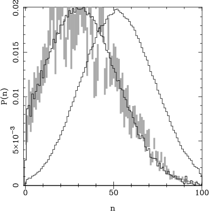
Figure 2: The output photon number distribution for a laser. The histogram with the error bars comes from a Quantum Jump simulation of a one atom laser. The other two histograms are obtained from the theories of Haake et al. [7] (histogram on the left) and Lugiato et al. [15] (histogram on the right). Note the agreement of the theory of Haake et al. with the numerical solution of the master equation. The laser parameters used in the simulation are $C=30;\ f=1;\ n_{s}=15;\ N=1;\ \sigma_{0}=0.05;\ \gamma t=\infty$.

In Fig. 2 we report a sample test with the detailed number probability distribution for the stationary state from the QJ method for a one-atom laser versus the results of simulations of the FPE of both Refs. [7] and [15]. One can see that in this regime the FPE of Ref. [7] perfectly reproduces results from the QJ, whereas there are discrepancies with results from the FPE of Ref. [15]. We have analyzed a wide range of parameters, and found always perfect agreement for the FPE (78), within the validity limits given in Subsec. 6.3.

7.2 Comparison between linear and saturable amplifiers

In this subsection we compare the ideal (i.e. with vacuum idler) PIA and the laser saturable amplifier described by the FPE (78). The amplifier is inserted in a binary communication channel, with the “0” bit encoded on the vacuum state $|0\rangle$ and the “1” bit encoded on a fixed coherent state $|\alpha\rangle$. We analyze the gain $G$, the noise figure $R$ and the bit error rate $B$. In the linear regime the laser is equivalent to a PIA with gain

$$G=\exp[2\gamma t(1-2\sigma_{0}C)]\;,$$ (88)

but with a non vacuum idler mode with number of photons

$$n_{b}=\frac{\mbox{min}\left\{C(1+\sigma_{0}),C(1-\sigma_{0})+1\right\}}{|2C\sigma_{0}-1|}.$$ (89)

From Eq. (88) one can see that the laser amplifies the radiation if the threshold condition $\sigma_{0}>1/2C$ is satisfied. The idler photons produce additional noise (see Eq. (58)) and the ideal PIA has always a better noise figure than the laser. Correspondingly, from numerical simulations we found that the ideal PIA also performs better than the laser in terms of BER. In the saturation regime, on the other hand, the noise figure of the laser can be much smaller than the 3-dB standard noise figure of the PIA, as assessed in Refs. [3],[20]. However, in such a regime, the noise figure $R$ is not the significant criterion of goodness to be considered, as explained in Sec. 4 and pointed out in Refs. [5] and [6]. As a matter of fact, the numerical analysis shows that the BER for the laser is always worse than (or, at best, very close to) that of the PIA, even if the noise figure for the laser is very small. The mechanism leading to such discrepancy between noise figure and BER criteria is illustrated in Fig. 3, where the output probability distribution of the two amplifiers is plotted in a regime of strong saturation for the laser.

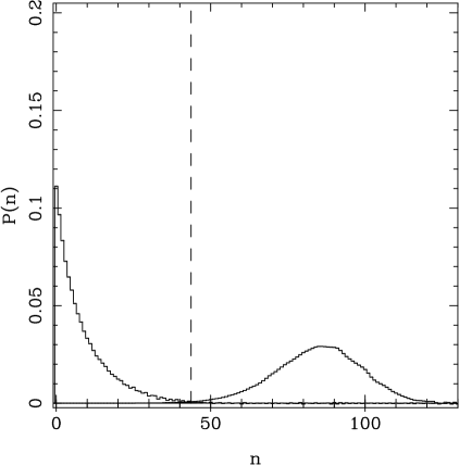
Figure 3: Comparison between the output photon number distributions $p_{n}$ of the saturable amplifier (left figure) and ideal PIA (right figure). The parameters used in this simulation are $C=4.5;\ n_{s}=N=55;\ \sigma_{0}=1;\ \gamma t=0.2;\ |\alpha|=3.95$ (amplitude of the input coherent state pertaining bit “1”). This amplifier has a gain of $6.873$ dB.

The saturated laser tends to cut off the right tail of the output distributions for high photon numbers. On the other hand, the ideal PIA, being a linear device, evolves both tails of the distribution in the same way. If we analyze the two amplifiers at the same gain, the left tail of the bit “1” distribution will be higher for the saturable laser than for the ideal PIA, since saturation needs a higher contribution from the left tail in order to achieve the same gain, and the left tail is less influenced by saturation than the right one. For the same reason the bit “0” distribution at the output of the laser turns out to be much more broadened than for the PIA. As a consequence the overlap region of the two (“0” and “1”) distributions – i.e. the bit error rate – is higher in the saturable laser than in the PIA.

8 Conclusions.

In this paper we have shown that, for direct detection, saturation effects in a traveling wave laser amplifier cannot yield BER better than those for a PIA, although they greatly reduce the noise figure greatly below the SQL of 3 dB. In fact, the saturation mechanism broadens the output probability distributions asymmetrically, in such a way that the noise figure is improved, whereas the overlap between the distributions, which gives the BER, is increased. This mechanism has been shown on the basis of a careful Monte Carlo simulation of a traveling wave laser amplifier. The question now is: is it possible to improve the BER of the PIA in some way? The answer is clearly affirmative, if one just considers that at least the ideal PNA could in principle achieve zero BER when amplifying input number states, or has $B=e^{-|\alpha|^{2}}$ independent of the gain $G$ for input bit “1” in the coherent state $|\alpha\rangle$, a value anyway much smaller than the corresponding BER for the PIA. Now the problem is how to achieve or to approach a PNA by a real device, and from the present analysis we conclude that the saturated laser does not approximate a PNA better than a PIA, even though it has a very low noise figure.

References

References

- 1 H. P. Yuen and M. Ozawa, Phys. Rev. Lett. 70, 363 (1993).
- 2 For example see: J.A. Levenson, I. Abram, Th. Rivera and Ph. Grangier, J. Opt. Soc. Am. B 10, 2233 (1993).
- 3 G. M. D’Ariano, C. Macchiavello, M. G. A. Paris, Phys. Rev. Lett. 73, 3187 (1994).
- 4 H. P. Yuen, Phys. Rev. Lett. 56, 2176 (1986).
- 5 O. Nilsson, A. Karlsson, J.-P. Poizat, E. Berglind, Phys. Rev. Lett. 76, 1972 (1996).
- 6 G. M. D’Ariano, C. Macchiavello, M. G. A. Paris, Phys. Rev. Lett. 76, 1973 (1996).
- 7 F. Haake, M. Lewenstein, Phys. Rev. A 27 1013 (1983).
- 8 C. W. Helstrom, Quantum Detection and Estimation Theory (Academic Press, New York, 1976).
- 9 H. P. Yuen, Phys. Lett. 91A, 101 (1982).
- 10 A. S. Holevo, Probl. Inf. Transm. 9, 177 (1973).
- 11 G. M. D’Ariano, C. Macchiavello and M. G. A. Paris, Information gain in quantum communication channels, in “Quantum Communications and Measurement”, ed. by V. P. Belavkin et al., Plenum Press, New York (1995), p.339.
- 12 E. B. Davies, Quantum theory of open systems, (Academic Press, London, New York, 1976).
- 13 G. Lindblad, Commun. Math. Phys. 48, 119 (1976).
- 14 G. M. D’Ariano, Phys. Lett. A 187, 231 (1994).
- 15 L. A. Lugiato, F. Casagrande and L. Pizzuto, Phys. Rev. A 26 3438 (1982).
- 16 K. Mølmer, Y. Castin, J. Dalibard, J. Opt. Soc. Am. B 10, 524 (1993)
- 17 R.Dum, P.Zoller and H.Ritsch, Phys. Rev. A 45, 4879 (1992).
- 18 G. M. D’Ariano, Phys. Rev. A 45, 3224 (1992)
- 19 G. M. D’Ariano, C. Macchiavello, S. Moroni, Mod. Phys. Lett. B 8, 239 (1994).
- 20 For the parameter choice exploited in Ref. [3] both theories of Haake [7] and Lugiato [15] give the same results.
- 21 G. M. D’Ariano, Int. J. Mod. Phys. B 6, 1291 (1992)
- 22 G. M. D’Ariano, C. Macchiavello, Phys. Rev. A 48, 3947 (1993)