Does Quantum Mechanics imply influences
acting backward in time
in impact series experiments?

Abstract

A real two-particle experiment is proposed in which one of the particles undergoes two successive impacts on beam-splitters. It is shown that the standard quantum mechanical superposition principle implies the possibility of influences acting backward in time (”retrocausation”), in striking contrast with the principle of causality. It is argued that nonlocality and retrocausation are not necessarily entangled.

Keywords: superposition principle, backward in time influences (retrocausation), superluminal nonlocality, multisimultaneous causality.

1 Introduction

Bell experiments with time-like separated impacts at the splitters have already been done [1] demonstrating the same correlations as for space-like separated ones. Consider such an experiment in which the measurement on particle $2$ lies time-like separated after the measurement on particle $1$. It is clear that at the time particle $1$ produces its outcome value, it cannot account for values of particle $2$ because such values do not exist at all, from any observer’s point of view. In this case which measurement is made first and which after dos not depend on the inertial frame. Therefore, in agreement with the principle that the effects cannot exist before the causes, it is reasonable to assume that the correlations appear because particle 1 chooses its outcome without being influenced by the choice particle 2 will make, and particle 2 chooses its outcome taking account of the choice particle 1 has made.

The impossibility of influences acting backward in time (the causality principle) is basic to any causal model, independently of one accepts or rejects the impossibility of superluminal influences (relativistic causality). In particular, the causality principle has been unified with the relativity of simultaneity in a consistent way to account for the superluminal nonlocal influences, and the consequent violation of relativistic causality, which happen in Bell experiments with space-like separated measuring devices. The resulting model is referred to as Relativistic Nonlocality (RNL) or Multisimultaneity [2, 3]. Assuming multisimultaneous causality, RNL is at odds with Lorentz-invariance [4]. And even though RNL agrees with QM for all experiments already done, both theories conflict in their predictions regarding new proposed experiments with fast moving polarizers.

The opposite view to the causal one is undoubtedly ”retrocausation”, i.e., the position admiting that decisions at present can influence the past. ”Retrocausation” has been developed as a consistent Lorentz-invariant interpretation of ordinary QM by O. Costa de Beauregard [5]. The discussion about the possibility of influences acting backwards in time has been recently stimulated by H. Stapp [6]. The ongoing controversy [7, 8, 9, 10] is highlighting that we have not yet found an specific experiment allowing us to decide between the causal view and retrocausation, in a similar way as Bell experiments allow us to decide between local realism and superluminal nonlocality.

In this paper a possible real experiment is discussed in which ordinary QM leads to predictions which imply influences backward into a timelike separated past, and therefore may contribute to clarify whether nature behaves retrocausal or not.

2 The experiment

Consider the setup sketched in Fig.1. Photon pairs are emitted through down-conversion from a source $S$. Photon 1 enters the left hand side interferometer and impacts on beam-splitter BS₁₁ before being detected in either D${}_{1}(+)$ or D${}_{1}(-)$, while photon 2 enters the 2-interferometer series on the right hand side impacting successively on BS₂₁ and BS₂₂ before being detected in either D${}_{2}(+)$ or D${}_{2}(-)$. Each interferometer consists in a long arm of length $L$, and a short one of length $l$. We assume as usual the path difference set to a value which largely exceeds the coherence length of the photon pair light, but which is still smaller than the coherence length of the pump laser light.

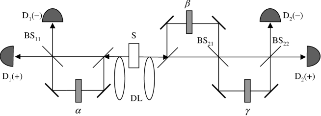
Figure 1: Impact series experiment with photon pairs: photon 2 impacts successively on beam-splitter BS₂₁ and BS₂₂. See text for detailed description.

For a pair of photons, eight possible path pairs lead to detection. We label them as follows: $(l,ll)$; $(L,ll)$; $(l,Ll)$ and so on; where, e.g., $(l,Ll)$ indicates the path pair in wich photon 1 has taken the short arm, and photon 2 has taken first the long arm, then the short one.

Ordinary QM assumes indistinguishability to be a sufficient condition for observing quantum interferences and entanglement, whereas RNL assumes this condition to be only a necessary one. In any case, as a first step we must distribute all possible paths in mutually distinguishable subensembles. The following table gives the four mutually distinguishable subensembles of the ensemble of all possible path pairs.

$$\begin{array}[]{lll}(l,LL)&:&2L-l\\ (L,LL)\,,\,(l,Ll)\,,\,(l,lL)&:&L\\ (l,ll)\,,\,(L,Ll)\,,\,(L,lL)&:&l\\ (L,ll)&:&2l-L\end{array}$$ (1)

where the right-hand side of the table indicates the path difference between the single paths of each photon characterising each subensemble of path pairs. From now on, unless stated otherwise, we consider only those events that are characterized by path difference $L$, i.e., $(L,LL)\,,\,(l,Ll)\,,\,(l,lL)$. Experimentally, this is done as usual by appropriate coincidence electronics [11].

By means of delay lines DL the impacts on BS₁₁ are set time-like separated from the impacts on BS₂₁ and BS₂₂. We are interested in two different time orderings:

1. The impact on BS₂₂ happens before the impact on BS₁₁.

2. The impact on BS₁₁ happens before the impact on BS₂₁.

3 The QM view

For reasons that will become clear in the next section we are not interested in the joint probabilities but in the single probabilities at each side of the setup, i.e., the probability of getting a count in detector D${}_{2}(\sigma)$ independently of where photon 1 is detected, which we denote $P^{QM}_{\pm\sigma}(L)$, and the probability of getting a count in detector D${}_{1}(\sigma)$ independently of where photon 2 is detected, which we denote $P^{QM}_{\sigma\pm}(L)$, where the $L$ in the parenthesis refers to the corresponding path difference.

The single probabilities are related to the conventional joint ones as follows:

$$\begin{array}[]{lll}P^{QM}_{\pm+}(L)\,\equiv\,P^{QM}_{++}(L)+P^{QM}_{-+}(L)\\ P^{QM}_{\pm-}(L)\,\equiv\,P^{QM}_{+-}(L)+P^{QM}_{--}(L)&\end{array}$$ (2)

and

$$\begin{array}[]{lll}P^{QM}_{+\pm}(L)\,\equiv\,P^{QM}_{++}(L)+P^{QM}_{+-}(L)\\ P^{QM}_{-\pm}(L)\,\equiv\,P^{QM}_{-+}(L)+P^{QM}_{--}(L)&\end{array}$$ (3)

Quantum mechanics is not time-ordering sensitive, and the superposition principle states for any possible time ordering:

$$P^{QM}_{\sigma\omega}(L) = \left|A_{\sigma\omega}(L,LL)+A_{\sigma\omega}(l,Ll)+A_{\sigma\omega}(l,lL)\right|^{2}$$ (4)

where $A_{\sigma\omega}(path)$, ($\sigma,\omega\in\{+,-\}$), denote the probability amplitudes for the path pair specified in the parenthesis and the outcome specified in the subscript. Substituting the amplitudes given in (17), (20) and (23) of the Appendix into Eq. (4) and adding according to (LABEL:eq:SPJP1) leads to the corresponding single probabilities for the detections at side 2 (right-hand side) of the setup:

$$\begin{array}[]{lll}P^{QM}_{\pm+}(L)&=&\frac{1}{2}+\frac{1}{3}\cos(\beta-\gamma)\\ P^{QM}_{\pm-}(L)&=&\frac{1}{2}-\frac{1}{3}\cos(\beta-\gamma)\end{array}$$ (5)

Adding according to (LABEL:eq:SPJP2) leads to the corresponding single probabilities for the detections at side 1 (left-hand side) of the setup:

$$\begin{array}[]{lll}P^{QM}_{+\pm}(L)&=&\frac{1}{2}-\frac{1}{3}\cos(\alpha+\beta)\\ P^{QM}_{-\pm}(L)&=&\frac{1}{2}+\frac{1}{3}\cos(\alpha+\beta)\end{array}\,$$ (6)

4 The causal view

According to the causal view, in experiments working with time orderings 1 or 2 (see Section 2) the photon impacting before must behave exclusively taking account of the local parameters, i.e., it cannot become influenced by the choices of the parameters the other photon meets at the other arm of the setup. This means for instance in the experiment described in [1] that the photon impacting before produce single counts equally distributed, in agreement with the predictions of QM and the observed results.

For reasons given in [2, 3] we consider in the following that the outcome values for detections after beam-splitter BS_ik are determined at the time of arrival at this beam-splitters, and not at the detectors watching the output ports of BS_ik.

Consider now an experiment with time ordering 2. We accept that whether photon 2 arriving at BS₂₁ or BS₂₂ undergoes a transmission or a reflection may depend on which choice photon 1 did in BS₁₁, and hence on which D${}_{1}(\sigma)$ it has been detected. However to admit that the transmitted output port in BS₂₁ corresponds necessarily to a short or a long arm in the interferometer means to accept retrocausation, for the physicist is always free to decide to shorten or lengthen the arm once photon 2 has made its choice. Accordingly we state the following condition:

Causality condition: The path length traveled by the photon impacting later does not depend on the outcome value produced by the photon impacting first.

This condition implies that the distribution of the counts in the single detectors produced by the photon impacting first, say photon 1, does not depend on the subensemble of path pairs in table (1) to which the event will belong once the detection of photon 2 has occurred. In other words, even if the measurement selects only those counts in the detectors D${}_{1}(\sigma)$ yielding path difference $L$ through coincidence with the counts in the detectors D${}_{2}(\omega)$, the measured distribution of the outcomes in D${}_{1}(\sigma)$ is the same as if it had been possible to perform the experiment nonselectively with only the three paths belonging to the subensemble $L$.

Taking account of this conclusion any causal model accepting the available observations on first order interferences leads to the following predictions:

Time ordering 1: After photon 2 impacts on BS₂₂ no ulterior detection makes it possible to distinguish between the paths (lL) and (Ll), but it is still possible to know whether photon 2 traveled path (LL) by detecting particle 1 before it impacts on BS₁₁. Therefore, if photon 2 behaves taking account only of local information, paths (lL) and (Ll) lead to first order interferences, and path (LL) does not interfere at all. The usual application of the sum-of-probability-amplitudes and the sum-of-probabilities leads to the relation:

$$P^{C}_{\pm\sigma}=\left|A_{\sigma}(LL)\right|^{2}+\left|A_{\sigma}(Ll)+A_{\sigma}(lL)\right|^{2}$$ (7)

where $P^{C}_{\pm\sigma}$ denotes the single probability of getting a count in detector D${}_{2}(\sigma)$ predicted by the causal view, and $A_{\sigma}(path)$ the amplitude associated with this detection for the single path of photon 2 specified in the parenthesis. Substituting according to (35), (38), and (41) in the Appendix one gets the following single probabilities for each detector D${}_{2}(\sigma)$:

$$\begin{array}[]{lll}P^{C}_{\pm+}&=&\frac{1}{2}+\frac{1}{3}\cos(\beta-\gamma)\\ P^{C}_{\pm-}&=&\frac{1}{2}-\frac{1}{3}\cos(\beta-\gamma)\end{array}$$ (8)

i.e. one gets the same probabilities as those predicted by QM in (5).

Time ordering 2: After the impact of photon 1 on BS₁₁ it is still possible to know whether it traveled path $L$ or $l$ by detecting photon 2 before it impacts on BS₂₁. Therefore photon 1 has to distribute its choices following the sum-of-probabilites rule and one is led to the following probabilities:

$$\begin{array}[]{lll}P^{C}_{+\pm}&=&\frac{1}{2}\\ P^{C}_{-\pm}&=&\frac{1}{2}\end{array}$$ (9)

which clearly contradicts the QM predictions in (6).

We would like to stress that the preceding result holds for any theory accepting the causality principle, i.e., the impossibility of influencing backward a timelike separated past. Obviously, one would like to know also which probabilities predicts the causal view for the single detections of photon 1 in time ordering 1, and of photon 2 in time ordering 2. Notice that first of all this point does not matter at all for our argument, and secondly these probabilities will depend on the particular causal model under consideration. As regards RNL or Mulsimultaneity [2, 3] we give an answer in Section 6 below.

5 Conflict between QM and Causality

As far as we know this is the first time in a two-particle experiment QM predicts single probabilities (6) for one of the particles which depend on parameters the other particle meets on the other side of the setup. The effect of retrocausation violating the principle of causality is plain because it occurs backward in time between timelike separated events.

Could such a retrocausation effect be used to built a time machine? Consider the single probabilities for the subensemble with path difference $l$ in Table (1). The superposition principle of QM states:

$$P^{QM}_{\sigma\omega}(l) = \left|A_{\sigma\omega}(l,ll)+A_{\sigma\omega}(L,Ll)+A_{\sigma\omega}(L,lL)\right|^{2}$$ (10)

Substituting the amplitudes of (26), (29) and (32) in the Appendix into Eq. (10) one gets:

$$\begin{array}[]{lll}P^{QM}_{+\pm}(L)&=&\frac{1}{2}+\frac{1}{3}\cos(\alpha+\beta)\\ P^{QM}_{-\pm}(L)&=&\frac{1}{2}-\frac{1}{3}\cos(\alpha+\beta)\end{array}\,$$ (11)

Eq. (6) and (11) together show that an observer watching only the detectors D₁ cannot become aware in the present of actions performed in the future of his light cone. However, according to QM the coincidences measurement should demonstrate such influences acting really backward in time. The similarity with the superluminal nonlocality implied by ordinary QM is impressive: in this case the coincidences measurement demonstrates real faster-than-light influences, even though these influences cannot be used for superluminal telegraphing.

6 The RNL or mulsimultaneous causal view

According to this theory [3] probabilities for counts in single detectors must depend exclusively on local information, i.e., they are the same for a before and a non-before impact. Since in the proposed experiment the sum-of-probability-amplitudes rule violates this principle, the probabilites have to be calculate applying sum-of-probabilities. In other words the violation of causality works in RNL in the same way as the violation of indistinguishability in QM. Accordingly (8) and (9) hold for the two considered time orderings, and also for any other time ordering in experiments with spacelike separated impacts: the presence of paths (lL) and (Ll) leading to first order interferences excludes in this case the second order ones.

Notice that RNL, though causal, is a specific nonlocal theory. That it conflicts with QM suggests that the issues of superluminal nonlocality and of retrocausation are not really entangled, and should be conceptually distinguished: Nothing speaks in principle against the possibility that Nature uses faster-than-light influences but avoids backward-in-time ones.

7 Real experiment

A real experiment can be carried out arranging the setup used in [1] in order that the photon traveling the long fiber of 4.3 km impacts on a second beam-splitter before it is getting detected. For the values:

$$\alpha+\beta=n\,\pi\,$$ (12)

with $n$ integer, the equations (6) and (8) yield the predictions:

$$E^{QM}=|P^{QM}_{+\pm}(L)-P^{QM}_{-\pm}(L)|=\frac{2}{3}$$

$$E^{C}=|P^{C}_{+\pm}(L)-P^{C}_{-\pm}(L)|=0$$ (13)

Hence, for settings according to (12) the experiment represented in Fig. 1 allow us to decide between quantum mechanics and the causal view through determining the experimental quantity:

$$E=\frac{R_{++}+R_{+-}-R_{-+}+R_{--}}{R_{++}+R_{+-}+R_{-+}+R_{--}},$$ (14)

where $R_{\sigma\omega}$ are the four measured coincidence counts in the detectors.

8 Conclusion

We have shown that in the proposed impact series experiment ordinary QM leads to influences backward in time, even if these influences cannot be used to build a time machine. If the experiment upholds QM, Costa de Beauregard’s and Stapp’s views would appear to be the correct way of interpreting QM, quite in agreement with Lorentz-invariance but in striking contradiction to the causality principle. If the experiment upholds causality, then Relativistic Non-Locality (RNL) or Multisimultaneity would receive strong support. In RNL, indistinguishability is no more a sufficient condition for entanglement, and both superluminal influences as well as the impossibility of influences acting backwards in time have the status of principles. Whatever the answer may be, the experiment is capable of bearing a promising controversy between QM and Causality, similar to the controversy between QM and Local Realism.

Appendix

In the following are listed the probability amplitudes of the path pairs and the single paths we are interested in.

8.1 Probability Amplitudes of the path pairs with length difference $L$ in Table (1)

We denote $A_{\sigma\omega}(\mbox{path})$ the probability amplitude associated to detection of photon 1 in $D_{1}(\sigma)$ and of photon 2 in $D_{2}(\omega)$, for the specified path. The probability amplitudes for the path pairs of subensemble $L$ in (1) normalized to only these three path pairs are:

$$(l,Ll) : \left\{\begin{array}[]{lllll}A_{++}(l,Ll)&=&-\,A_{--}(l,Ll)&=&-\frac{1}{\sqrt{3}}\,\frac{1}{2}\,e^{i\beta}\\ A_{+-}(l,Ll)&=&A_{-+}(l,Ll)&=&-i\,\frac{1}{\sqrt{3}}\,\frac{1}{2}\,e^{i\beta}\end{array}\right.$$ (17)

$$(l,lL) : \left\{\begin{array}[]{lllll}A_{++}(l,lL)&=&A_{--}(l,lL)&=&-\frac{1}{\sqrt{3}}\,\frac{1}{2}\,e^{i\gamma}\\ A_{+-}(l,lL)&=&-\,A_{-+}(l,lL)&=&i\,\frac{1}{\sqrt{3}}\,\frac{1}{2}\,e^{i\gamma}\end{array}\right.$$ (20)

$$(L,LL) : \left\{\begin{array}[]{lllll}A_{++}(L,LL)&=&-\,A_{--}(L,LL)&=&\frac{1}{\sqrt{3}}\,\frac{1}{2}\,e^{i(\alpha+\beta+\gamma)}\\ A_{+-}(L,LL)&=&A_{-+}(L,LL)&=&-i\,\frac{1}{\sqrt{3}}\,\frac{1}{2}\,e^{i(\alpha+\beta+\gamma)}\end{array}\right.$$ (23)

8.2 Probability Amplitudes of the path pairs with length difference $l$ in Table (1)

The probability amplitudes for the path pairs of subensemble $l$ in (1) normalized to only these three path pairs are:

$$(l,ll) : \left\{\begin{array}[]{lllll}A_{++}(l,ll)&=&-\,A_{--}(l,ll)&=&\frac{1}{\sqrt{3}}\,\frac{1}{2}\\ A_{+-}(l,ll)&=&A_{-+}(l,ll)&=&\frac{1}{\sqrt{3}}\,\frac{1}{2}\,i\end{array}\right.$$ (26)

$$(L,lL) : \left\{\begin{array}[]{lllll}A_{++}(L,lL)&=&-\,A_{--}(L,lL)&=&\frac{1}{\sqrt{3}}\,\frac{1}{2}\,e^{i(\alpha+\gamma)}\\ A_{+-}(L,lL)&=&A_{-+}(L,lL)&=&-\,\frac{1}{\sqrt{3}}\,\frac{1}{2}\,i\,e^{i(\alpha+\gamma)}\end{array}\right.$$ (29)

$$(L,Ll) : \left\{\begin{array}[]{lllll}A_{++}(L,Ll)&=&A_{--}(L,Ll)&=&\frac{1}{\sqrt{3}}\,\frac{1}{2}\,e^{i(\alpha+\beta)}\\ A_{+-}(L,Ll)&=&-\,A_{-+}(L,Ll)&=&\frac{1}{\sqrt{3}}\,\frac{1}{2}\,i\,e^{i(\alpha+\beta)}\end{array}\right.$$ (32)

8.3 Probability Amplitudes of the single paths $LL$, $Ll$, $lL$ traveled by photon 2 in the proposed experiment

We denote $A_{\sigma}(\mbox{path})$ the probability amplitude associated to detection of photon 2 in D${}_{2}(\sigma)$, for the specified path. The probability amplitudes for the paths $LL$, $Ll$, $lL$ photon 2 travels in an experiment selecting the path pairs with path difference $L$ in (1), normalized as if the experiment were performed with only these three paths are:

$$(Ll) : \left\{\begin{array}[]{lll}A_{+}(Ll)&=&-\frac{1}{\sqrt{3}}\frac{1}{\sqrt{2}}\,e^{i\beta}\\ A_{-}(Ll)&=&-i\,\frac{1}{\sqrt{3}}\frac{1}{\sqrt{2}}\,e^{i\beta}\end{array}\right.$$ (35)

$$(lL) : \left\{\begin{array}[]{lll}A_{+}(lL)&=&-\frac{1}{\sqrt{3}}\frac{1}{\sqrt{2}}\,e^{i\gamma}\\ A_{-}(lL)&=&i\,\frac{1}{\sqrt{3}}\frac{1}{\sqrt{2}}\,e^{i\gamma}\end{array}\right.$$ (38)

$$(LL) : \left\{\begin{array}[]{lll}A_{+}(LL)&=&-\frac{1}{\sqrt{3}}\frac{1}{\sqrt{2}}\,e^{i(\beta+\gamma)}\\ A_{-}(LL)&=&i\,\frac{1}{\sqrt{3}}\frac{1}{\sqrt{2}}\,e^{i(\beta+\gamma)}\end{array}\right.$$ (41)

References

- [1] P.R. Tapster, J.G. Rarity and P.C.M. Owens Phys.Rev.Lett., 73 (1994) 1923-1926.
- [2] A. Suarez and V. Scarani, Phys. Lett. A 232 (1997) 9-14, and quant-ph/9704038.
- [3] A. Suarez Phys. Lett. A 236 (1997) 383-390 and quant-ph/9711022.
- [4] A. Suarez and V. Scarani Phys. Lett. A 236 (1997) 605-606.
- [5] O. Costa de Beauregard Phys. Lett. A 236 (1997) 602-604, and references therein.
- [6] H. Stapp, American Journal of Physics, 65 (1997) 300-304, and: quant-ph/9711060, quant-ph/9801056.
- [7] W.G. Unruh, Is Quantum Mechanics Non-Local?,quant-ph/9710032.
- [8] N.D. Mermin, Nonlocality and Bohr’s reply to EPR, quant-ph/9712003.
- [9] J. Finkelstein, Yet another comment on ”Nonlocal character of quantum theory”, quant-ph/9801011.
- [10] V.S. Mashkevich, On Stapp-Unruh-Mermin Discussion on Quantum Nonlocality, quant-ph/9801032.
- [11] W. Tittel, J. Brendel, B. Gisin, T. Herzog, H. Zbinden, and N. Gisin quant-ph/9707042.