Transverse mode coupling in a Kerr medium

Abstract

We analyze non-linear transverse mode coupling in a Kerr medium placed in an optical cavity and its influence on bistability and different kinds of quantum noise reduction. Even for an input beam which is perfectly matched to a cavity mode, the non-linear coupling produces an excess noise in the fluctuations of the output beam. Intensity squeezing seems to be particularly robust with respect to mode coupling while quadrature squeezing is more sensitive. However it is possible to find a mode the quadrature squeezing of which is not affected by the coupling.
PACS number(s): 42.65.Sf

I Introduction

During the last years different kinds of systems for the generation of squeezed light have been proposed and realized. The bistable device obtained by placing a non-linear Kerr medium inside an optical cavity is one of them. When the bistability turning point is approached, the fluctuations in one of the field quadratures of the incoming beam are reduced below shot noise [1, 2, 3, 4]. Nearly perfect squeezing is expected when the non-linear medium is a lossless Kerr medium [5, 6, 7]. Squeezing via the optical Kerr effect was experimentally demonstrated at the output of a bistable cavity containing an atomic beam[8, 9] or a cloud of cold atoms released from a magneto-optical trap [10].

Most theoretical treatments have simplified the description of the field-matter interaction by modeling the laser beam as a plane-wave [1-7]. Thanks to these works, the squeezing mechanism in this system is well understood and it has been shown that this kind of device has the potential to generate very large squeezing. There is now a need for more complete models, either to analyze experimental results of current experiments or to estimate the limitations of future set-ups. For more realistic systems it is clear that the plane wave description has to be modified to account for the spatial structure of the laser beam. When dealing with a non-linear medium made of atoms, a first step consists in averaging the mean field as well as the fluctuations over the beam profile in order to take into account the differences of light intensity and of coupling strength at different localizations inside the beam [11, 12, 13, 14]. This leads to a modification of the bistability curve and of the squeezing obtainable with the device. Only in the limit of an ideal Kerr medium (characterized by a $\chi^{\left(3\right)}$ susceptibility) this single transverse mode approach leads to results identical to the plane wave model [14].

It is also well known that the interaction of a light beam with a non-linear medium gives rise to transverse spatial effects which may have a strong influence on the quantum fluctuations of the beam [15, 16]. For a Kerr medium, the first effects of the non-linearity (before the appearance of spatial instabilities) are self focusing or self defocusing. When dealing with a medium inside an optical cavity, these effects produce a coupling between different transverse modes, which depends on the intracavity intensity and changes not only the mean field but also field fluctuations. In particular the non-linear coupling produces an excess noise which is appreciable even if the cavity is perfectly matched to the spatial structure of the input beam. The existence of this coupling is of course well known, and most of the time cavities are designed to avoid a degeneration between a transverse mode and the fundamental mode of the cavity. Single mode operation is thus achieved. However, as we will show in this paper, transverse modes have to be taken into account even for an input mode which is perfectly matched to the fundamental mode of a nondegenerate cavity. We will evaluate their effect on the quantum noise reduction and show that they can constitute a limiting factor for squeezing obtainable in the fundamental mode.

We study in particular the influence of higher order transverse cavity modes on optical bistabilty and on different kinds of quantum noise reduction. The calculations are based on a linear input-output formalism where fluctuations are linearized around the working point of the system [17]. We describe the spatial beam structure in terms of Gauss-Laguerre modes. The effect of the Kerr non-linearity is then a coupling between the transverse modes. In section II, we derive the coupling coefficients between the modes for a light beam propagating through a thin Kerr medium. To present our approach we study in section III the propagation through a thin medium in free space. The modes coupling is at the origin of non-linear losses for the fundamental mode. We show that the fluctuations associated to these losses are not vacuum fluctuations but correspond to phase conjugated noise. In section IV we consider a Kerr medium inside an optical cavity. We derive analytic expressions for the excess noise produced in the fundamental mode through the coupling to higher order modes. In free space, this excess noise can not be neglected since its strength is of the same order of magnitude than the strength of the parametric noise modification. However, if the Kerr medium is placed in a cavity, the cavity provides a mode selection which can lead to an important reduction of the perturbing effect of higher order transverses modes on the fundamental mode. When the cavity is non degenerate and the transverse mode spacing is large compared to the cavity width, one can perform a perturbative treatment in order to evaluate the influence of transverse mode coupling on the fundamental cavity mode. The fundamental mode may also accidentally coincide with a higher order mode corresponding to an other longitudinal mode family. In this case, one can calculate steady state and fluctuations by performing a two mode approximation described in the second part of section IV. The analysis of transverse mode coupling will finally enable us to estimate the validity limit of a single mode approximation. The discussion of the results as well as some conclusive remarks will be presented in section V. Details of the calculations are exposed in the appendix.

II Nonlinear coupling of Gauss-Laguerre modes in a Kerr medium

In this section, we study the propagation of a light beam of arbitrary transverse shape through a thin Kerr medium. The analysis will supply us with the coupling coefficients between different transverse modes due to non-linear coupling. We consider a light beam of frequency $\omega_{{\rm L}}$ which is described by the complex amplitude $E\left({\bf r}\right)$ of the electric field where ${\bf r}$ stands for the three-dimensional position $\left(r,\theta,x\right)$ in cylindrical coordinates:

$${\cal E}\left({\bf r}\right)=e^{-i\omega_{L}t}E\left({\bf r}\right)+e^{i\omega_{L}t}E\left({\bf r}\right)^{\dagger}.$$ (1)

In the paraxial approximation, the propagation of the field amplitude along the $x$ direction is given by

$$\triangle_{{}_{\perp}}E\left({\bf r}\right)+2ik_{L}\frac{\partial E\left({\bf r}\right)}{\partial x}=-\frac{k_{L}^{2}}{\varepsilon_{0}}P_{{\rm NL}}\left({\bf r}\right).$$ (2)

$P_{{\rm NL}}\left({\bf r}\right)$ is the non-linear polarization of the medium, $\triangle_{{}_{\perp}}$ stands for the transverse Laplacian and $k_{L}=\omega_{{\rm L}}/c$ is the light wavevector. The electric field may be expanded in Gauss-Laguerre modes $u_{p}^{\left(l\right)}\left({\bf r}\right)$ which are solutions of the propagation equation in free space in cylindrical coordinates:

$$E\left({\bf r}\right) = \sum_{p,l}A_{p}^{\left(l\right)}\left(x\right)u_{p}^{\left(l\right)}\left({\bf r}\right),$$ (3)

$$u_{p}^{\left(l\right)}\left({\bf r}\right) = \sqrt{\frac{2}{\pi}}\sqrt{\frac{n!}{\left(n+l\right)!}}\frac{1}{w\left(x\right)}\left(\sqrt{2}\frac{r}{w\left(x\right)}\right)^{l}$$ (5)

$$\times L_{p}^{\left(l\right)}\left(2\frac{r^{2}}{w^{2}\left(x\right)}\right)\exp\left[-\frac{r^{2}}{w^{2}\left(x\right)}-i\varphi_{p}^{\left(l\right)}\left({\bf r}\right)\right].$$

$L_{p}^{\left(l\right)}$ is the generalized Laguerre polynomial, $\varphi_{p}^{\left(l\right)}\left({\bf r}\right)$ is the phase of the mode, $\lambda$ is the laser wavelength, $w\left(x\right)$ the beam size, $w_{0}$ the beam waist and $l_{R}$ the Rayleigh divergence length:

$$\varphi_{p}^{\left(l\right)}\left({\bf r}\right) = -\frac{\pi}{\lambda}\frac{x}{x^{2}+l_{R}^{2}}r^{2}+l\theta$$ (7)

$$+\left(2p+l+1\right){\arctan}\left(\frac{x}{l_{R}}\right),$$

$$w^{2}\left(x\right) = w_{0}^{2}\left(1+\frac{x^{2}}{l_{R}^{2}}\right),$$ (8)

$$l_{R} = \frac{\pi w_{0}^{2}}{\lambda}.$$ (9)

The fundamental Gaussian mode (TEM₀₀) corresponds to the indices $p=0$ and $l=0$. With the help of the normalization relations for Gauss-Laguerre modes[18] one can derive the propagation equation for the mode amplitudes $A_{p}^{\left(l\right)}\left(x\right)$ in presence of a dielectric medium:

$$\frac{\partial A_{p}^{\left(l\right)}\left(x\right)}{\partial x}=\frac{1}{2ik_{L}}\int dr\ d\theta\ u_{p}^{\left(l\right)}\left({\bf r}\right)^{*}P\left({\bf r}\right).$$ (10)

We will now assume the non-linearity to be represented by a lossless Kerr medium. The polarization $P\left({\bf r}\right)$ in this medium can be expressed through the non-linear susceptibility:

$$P_{{\rm NL}}\left({\bf r}\right)=\varepsilon_{0}\chi^{\left(3\right)}\left|E\left({\bf r}\right)\right|^{2}E\left({\bf r}\right).$$ (11)

From equation (10) we deduce the propagation equation for the field amplitudes

$$\frac{\partial A_{p}^{\left(l\right)}\left(x\right)}{\partial x} = i\frac{k_{L}\chi^{\left(3\right)}}{2}\sum_{mno,qrs}\Lambda_{pqrs}^{\left(lmno\right)}\left(x\right)A_{q}^{\left(m\right)}\left(x\right)^{*}$$ (13)

$$\times A_{r}^{\left(n\right)}\left(x\right)A_{s}^{\left(o\right)}\left(x\right),$$

where we have introduced the coupling coefficients $\Lambda_{pqrs}^{\left(lmno\right)}\left(x\right)$ between different modes:

$$\Lambda_{pqrs}^{\left(lmno\right)}\left(x\right) = \frac{1}{\pi w^{2}}\lambda_{pqrs}^{\left(lmno\right)}\delta_{l+m,n+o}$$ (15)

$$\times\exp\left[-2i\left(p+q-r-s\right)\arctan\left(\frac{x}{l_{R}}\right)\right],$$

$$\lambda_{pqrs}^{\left(lmno\right)} = 2\int_{0}^{\infty}dv\ v^{l+m}L_{p}^{\left(l\right)}\left(v\right)L_{q}^{\left(m\right)}\left(v\right)L_{r}^{\left(n\right)}\left(v\right)L_{s}^{\left(o\right)}\left(v\right)$$ (17)

$$\times\exp\left[-2v\right].$$

The dimensionless coefficients $\lambda_{pqrs}^{\left(lmno\right)}$ can be evaluated with the use of generating functions. Details of the calculation are exposed in appendix (A). In expression (15), one notices the presence of a selection rule $l+m=n+o$ which is due to the revolution symmetry of the problem. When a circularly symmetric beam ($l=0$) is sent into the medium, one can deduce from propagation equation (13) that it will only couple to higher order modes having the same (circular) symmetry. In this case, we will drop the index $l$

$$u_{p}\left({\bf r}\right) = u_{p}^{\left(0\right)}\left({\bf r}\right),$$ (18)

$$\lambda_{pqrs} = \lambda_{pqrs}^{\left(0000\right)}.$$ (19)

In this discussion we have neglected the effect of transverse instabilities, which arise in some region of parameter space[15], especially for high intensities, which we do not want to treat here.

III Field propagation in free space

We will now apply the treatment of non-linear coupling developed in the previous section to the propagation of a fundamental Gaussian mode through a Kerr medium. In order to simplify calculations we will consider a particular situation which is however often encountered in experiments. We assume the length $L$ of the medium to be much shorter than the Rayleigh divergence length. If the medium is placed in the beam waist, equation (13) for the propagation of the mode amplitudes simplifies to

$$\frac{\partial A_{p}\left(x\right)}{\partial x} = i\frac{\hat{K}}{L}\sum_{qrs}\lambda_{pqrs}A_{q}\left(x\right)^{*}A_{r}\left(x\right)A_{s}\left(x\right),$$ (20)

$$\hat{K} = \frac{k\chi^{\left(3\right)}L}{2\pi w^{2}}.$$ (21)

Let the amplitude of the incoming beam be $A_{{\rm in}}$. We will now study perturbatively the propagation of the fundamental mode inside the medium in the limit of a small non-linearity, that is $\hat{K}\left|A_{{\rm in}}\right|^{2}\ll 1$, condition which avoids the build-up of transverse instabilities. The calculation will be performed up to second order in the input intensity. Only in zero order the fundamental mode propagates undisturbed. Solving propagation equation (20) in iterative steps up to second order leads to the following expression for the fundamental mode amplitude after propagation through the medium

$$A_{0}\left(L\right) = \left[1+i\varphi_{{\rm NL}}-\frac{1}{2}\varphi_{{\rm NL}}^{2}-\frac{1}{2}\gamma_{{\rm NL}}\right]A_{{\rm in}},$$ (22)

$$\varphi_{{\rm NL}} = \hat{K}\left|A_{{\rm in}}\right|^{2},$$ (23)

$$\gamma_{{\rm NL}} = \frac{1}{3}\varphi_{{\rm NL}}^{2}.$$ (24)

In first order, the effect of the Kerr medium is a non-linear phase shift $\varphi_{{\rm NL}}$ proportional to the light intensity, like in the single mode approximation. After isolating the second order contribution of the non-linear phase shift, one notices also a non-linear loss term $\gamma_{{\rm NL}}$ due to the energy transfer into higher order modes. It has to be noted that as soon as the non-linear phase shift becomes important, the associated losses can not be neglected and a perturbative treatment of the coupling between the modes does not hold anymore.

Before calculating the propagation of fluctuations we will briefly introduce our notation and the input-output formalism. A detailed presentation of this method can be found in [19]. We will denote $\alpha_{p}$ the fluctuation amplitude of mode $p$ ($\alpha_{p}^{*}$ for its conjugate). To simplify notations it is convenient to use a vectorial notation where fluctuations of the light beam are completely described by a vector $\overrightarrow{\alpha}_{p}$ containing the two complex amplitudes:

$$\overrightarrow{\alpha}_{p}=\left[\begin{array}[]{c}{\cal\alpha}_{p}\\ {\cal\alpha}_{p}^{*}\end{array}\right].$$ (25)

We recall here that we will use a linear treatment of the fluctuations around the working point of the system. All relations for the complex amplitudes are therefore identical to the corresponding relations for the annihilation and creation operators $a_{p}$ and $a_{p}^{\dagger}$ of mode $p$. Fluctuations are characterized by their correlation functions $C_{\alpha\beta}\left(\tau\right)$:

$$C_{\alpha\beta}\left(\tau\right)=\left\langle\alpha\left(t+\tau\right)\beta\left(t\right)\right\rangle$$ (26)

The brackets correspond to the quantum mechanical expectation value. To calculate the explicit expressions for correlation functions it is convenient to consider the problem in Fourier space. Transformations between frequency and time domain are defined in the following way:

$$f\left[\omega\right]=\int dtf\left(t\right)e^{i\omega t}.$$ (27)

The Wiener Kinchin theorem establishes a relation between time and frequency dependent correlation functions:

$$\left\langle\alpha\left[\omega\right]\beta\left[\omega^{\prime}\right]\right\rangle = 2\pi\delta\left(\omega+\omega^{\prime}\right)C_{\alpha\beta}\left[\omega\right]$$ (28)

$$= 2\pi\delta\left(\omega+\omega^{\prime}\right)\int d\tau C_{\alpha\beta}\left(\tau\right)e^{i\omega\tau}.$$ (29)

Therefore fluctuations of a given mode may be completely described with the help of the following $2\times 2$ matrix $\underline{V}_{p}$ which contains all four field autocorrelation functions:

$\displaystyle\underline{V}_{p}\left[\omega\right]=\left[\begin{array}[]{cc}C_{{\cal\alpha}_{p}{\cal\alpha}_{p}^{*}}\left[\omega\right]&C_{{\cal\alpha}_{p}{\cal\alpha}_{p}}\left[\omega\right]\\ C_{{\cal\alpha}_{p}^{*}{\cal\alpha}_{p}^{*}}\left[\omega\right]&C_{{\cal\alpha}_{p}^{*}{\cal\alpha}_{p}}\left[\omega\right]\end{array}\right].$

After this brief introduction we will now consider the propagation of quantum fluctuations inside a Kerr medium. To this aim we will first derive a propagation equation for fluctuations of mode $p$ using the propagation equation for the mean field. Differentiating equation (20) leads to:

$$\frac{\partial\alpha_{p}}{\partial x}=i\frac{\hat{K}}{L}\sum_{qrs}\lambda_{pqrs}\left[A_{r}A_{s}\alpha_{q}^{*}+2A_{q}^{*}A_{r}\alpha_{s}\right].$$ (30)

In the case of a small non-linearity we develop the stationary mean field of the fundamental mode up to second order and obtain a perturbative solution for the modification $d\alpha_{0}$ of its fluctuations, which may be written as the sum of a parametric term $\left.d\alpha_{0}\right|_{{\rm par}}$ and additional fluctuations $\left.d\alpha_{0}\right|_{{\rm add}}$ coming from higher order modes:

$$d\alpha_{0} = \left.d\alpha_{0}\right|_{{\rm par}}+\left.d\alpha_{0}\right|_{{\rm add}},$$ (31)

$$\left.d\alpha_{0}\right|_{{\rm par}} = i\varphi_{{\rm NL}}\left(2\alpha_{0}+\alpha_{0}^{*}\right)-\frac{\varphi_{{\rm NL}}^{2}}{3}\left(3\alpha_{0}+2\alpha_{0}^{*}\right),$$ (32)

$$\left.d\alpha_{0}\right|_{{\rm add}} = 2i\varphi_{{\rm NL}}\sum_{q}\lambda_{q}\alpha_{q}+i\varphi_{{\rm NL}}\sum_{q}\lambda_{q}\alpha_{q}^{*}$$ (34)

$$-\frac{3}{2}\varphi_{{\rm NL}}^{2}\sum_{qr}\lambda_{q}\lambda_{qr}\alpha_{r}-\varphi_{{\rm NL}}^{2}\sum_{qr}\lambda_{q}\lambda_{qr}\alpha_{r}^{*}.$$

For simplicity we have assumed the incoming field amplitude $A_{{\rm in}}$ to be real. The parametric term may be readily obtained by differentiating equation (22). It corresponds to the usual parametric change of quantum fluctuations and is obtained similarly in the single mode approximation. The additional fluctuations can be understood as a consequence of the losses experienced by the fundamental mode due to its coupling to higher order modes. They correspond mainly to phase conjugated noise. Indeed in first order, they may be written as:

$$\left.d\alpha_{0}\right|_{{\rm add}}=i\varphi_{{\rm NL}}\sum_{q}\lambda_{q}\left(2\alpha_{q}+\alpha_{q}^{*}\right).$$ (35)

Their correlation function

$$\underline{V}_{{\rm add}}=\frac{1}{3}\hat{K}^{2}|A_{{\rm in}}|^{4}\left(\begin{array}[]{cc}4&-2\\ -2&1\end{array}\right)$$ (36)

is characteristic of the mode coupling by the Kerr medium and we will find it again in the following. Notice that even for small non-linearities this additional noise is never negligible.

IV Field propagation inside a bistable cavity

We come now to the case where the non-linear medium is not in free space but placed inside an optical cavity. We will consider the input field to be perfectly matched to the fundamental Gaussian mode of the cavity ($p=l=0$ for the input beam). Inside the cavity higher order transverse modes become important due to non-linear coupling. However, because of the cylindrical symmetry of the problem, we do not have to consider higher order modes with non-circular symmetry ($l\neq 0$). The cavity is supposed to be single ended, with an input mirror of amplitude transmissivity $\sqrt{2\gamma}$. In the limit of a high finesse cavity it is possible to derive an evolution equation for the intracavity field amplitude by evaluating the modification of the field during one roundtrip. The roundtrip propagation of the transverse mode $n,p$ gives rise to a phase shift $\varphi_{n,p}=\varphi_{0}+n\varphi_{{\rm L}}+p\varphi_{{\rm T}}$ which is the sum of the detuning $\varphi_{0}$ of the fundamental mode and integer multiple of the longitudinal phase spacing $\varphi_{{\rm L}}$ and the transverse phase spacing $\varphi_{{\rm T}}$ between different transverse modes. In a first approach, we will suppose the spacing between longitudinal modes to be much larger than $\varphi_{{\rm T}}$. In this limit, only one family of modes corresponding a longitudinal index $n_{0}$ has to be considered. This assumption will be given up in the last section, where we will consider also the influence of different longitudinal cavity modes.

Compared to the case of field propagation through a non-linear medium placed in free space, the field evolution equation inside the cavity has now to contain additional terms which take into account losses of the intracavity field as well as transmission of the input field through the cavity coupling mirror:

$$\tau_{c}\frac{dA_{p}(t)}{dt} = \sqrt{2\gamma}A_{p}^{{\rm in}}(t)-\left(\gamma+i\varphi_{p}\right)A_{p}(t)$$ (38)

$$\times+i\hat{K}\sum_{qrs}\lambda_{pqrs}A_{q}^{*}(t)A_{r}(t)A_{s}(t).$$

$\tau_{c}$ is the roundtrip time of the field inside the cavity. In the last term one recognizes the field modification due to the presence of the Kerr medium. For an empty cavity at resonance, the mean amplitude of the fundamental mode is $A_{\max}=\sqrt{2/\gamma}A^{{\rm in}}$ where the mean amplitude of the fundamental mode is $A^{{\rm in}}=\left\langle A_{0}^{{\rm in}}\right\rangle$. We can then define normalized mode amplitudes ${\cal A}_{p}=A_{p}/A_{\max}$, ${\cal A}_{p}^{{\rm in}}=A_{p}^{{\rm in}}/A^{{\rm in}}$ and ${\cal A}_{p}^{{\rm out}}=A_{p}^{{\rm out}}/A^{{\rm in}}$ respectively for the intracavity, input and output fields. They obey a dimensionless evolution equation

$$\frac{d{\cal A}_{p}}{d\tau}={\cal A}_{p}^{in}-\left(1+i\phi_{p}\right){\cal A}_{p}+iK\sum_{qrs}\lambda_{pqrs}{\cal A}_{q}^{*}{\cal A}_{r}{\cal A}_{s},$$ (39)

where $\tau=\gamma t/\tau_{{\rm c}}$ is a dimensionless time, $\phi_{p}=\varphi_{p}/\gamma$ is the normalized phase shift of mode $p$ and $K=\hat{K}\left|A_{\max}\right|^{2}/\gamma$ the normalized non-linear coupling coefficient. The output field is given as a sum of the reflected input field and the transmitted intracavity field:

$${\cal A}_{p}^{{\rm out}}(t)=-{\cal A}_{p}^{{\rm in}}(t)+2{\cal A}_{p}(t).$$ (40)

In a single mode approximation, the intracavity intensity exhibits bistable behaviour because of the intensity dependent phase shift. This phenomenon occurs as soon as the non-linear phase shift $\phi_{{\rm NL}}$ of the field is of the same order than the cavity width $\gamma$. Expressed with the dimensionless non-linear coupling coefficient $K$ the corresponding condition is $K\gtrsim 1$.

The evolution equation for the fluctuations is obtained by differentiating equation (39) for the mode amplitudes around the stationary working point

$$\partial_{\tau}{\cal\alpha}_{p} = {\cal\alpha}_{p}^{{\rm in}}-\left(1+i\phi_{p}\right){\cal\alpha}_{p}$$ (42)

$$+iK\sum_{qrs}\lambda_{pqrs}\left({\bar{{\cal A}}}_{r}{\bar{{\cal A}}}_{s}{\cal\alpha}_{q}^{*}+2{\bar{{\cal A}}}_{r}^{*}{\bar{{\cal A}}}_{s}{\cal\alpha}_{q}\right).$$

${\bar{{\cal A}}}_{r}$ is the stationary intracavity amplitude of mode $p$. Although we consider an input field which is spatially matched to the fundamental cavity mode, we nevertheless have to take into account fluctuations entering the cavity through all possible input modes. The output fluctuations can be deduced from

$${\cal\alpha}_{p}^{{\rm out}}=-{\cal\alpha}_{p}^{{\rm in}}+2{\cal\alpha}_{p}.$$ (43)

We have denoted here ${\cal\alpha}_{p}$, ${\cal\alpha}_{p}^{{\rm in}}$ and ${\cal\alpha}_{p}^{{\rm out}}$ the fluctuations of the normalized amplitudes ${\cal A}_{p}$, ${\cal A}_{p}^{{\rm in}}$ and ${\cal A}_{p}^{{\rm out}}$.

A Multimode perturbative approximation

As mentioned in the beginning of this section we will first consider the case where the transverse mode spacing is large compared to the cavity bandwidth. ($\phi_{{\rm T}}=\varphi_{{\rm T}}/\gamma\gg 1$). Hence, when the fundamental mode is nearly resonant, higher order transverse modes are far off resonance and their amplitudes will be small compared to the amplitude of the fundamental mode. This situation allows one to adopt a perturbative treatment of the coupling between fundamental and higher order modes, where the latter enter as first order quantities. Equation (39) can now be solved in iterative steps up to second order in the fundamental mode amplitude which leads to the new stationary state:

$$1 = \left[\left(1+\mu_{2}\frac{K^{2}{\cal A}_{0}^{4}}{\phi_{{\rm T}}^{2}}\right)+i\left(\phi_{0}-K{\cal A}_{0}^{2}-3\mu_{1}\frac{K^{2}{\cal A}_{0}^{4}}{\phi_{T}}\right.\right.$$ (45)

$$\left.\left.+3\mu_{2}\frac{\phi_{0}K^{2}{\cal A}_{0}^{4}}{\phi_{T}^{2}}-15\mu_{3}\frac{K^{3}{\cal A}_{0}^{6}}{\phi_{{\rm T}}^{2}}\right)\right]{\cal A}_{0},$$

$$\mu_{1} = \sum_{p\neq 0}\frac{\lambda_{p}^{2}}{p}=\ln\left(\frac{4}{3}\right)\simeq 0.288,$$ (46)

$$\mu_{2} = \sum_{p\neq 0}\frac{\lambda_{p}^{2}}{p^{2}}\simeq 0.268,$$ (47)

$$\mu_{3} = \sum_{p,q\neq 0}\frac{\lambda_{p}\lambda_{q}\lambda_{pq}}{pq}\simeq 0.197.$$ (48)

$\phi_{0}$ is the normalized linear phase shift. The first bracket gives the loss in the fundamental mode due to energy transfer to higher order modes. The last three terms in the second bracket describe the non-linear phase shift of the fundamental mode by the presence of higher order modes. Energy transfer and phase shift arise as soon as higher order transverse modes exist, but they are the smaller the more distant the perturbing transverse modes are from a cavity resonance. However, they increase with increasing intensity in the fundamental mode. At lowest order, their expressions are given by

$$\phi_{{\rm NL}} = \frac{\varphi_{{\rm NL}}}{\gamma}=K|{\cal A}_{0}|^{2},$$ (49)

$$\frac{\gamma_{{\rm NL}}}{\gamma} = \mu_{2}\frac{K^{2}|{\cal A}_{0}|^{4}}{\phi_{{\rm T}}^{2}}=\mu_{2}\frac{\phi_{{\rm NL}}^{2}}{\phi_{{\rm T}}^{2}}.$$ (50)

By comparing this relation to the free space situation (cf. equation (24)), one notices that the relations depend now on the cavity width $\gamma$ as well as on the transverse mode spacing $\phi_{{\rm T}}$. In general the cavity may therefore suppress or enhance the non-linear losses depending on whether the fundamental mode and higher order modes are degenerate or not. For the non degenerate cavity that we consider here the cavity reduces the non-linear losses considerably.

We will now discuss the treatment of fluctuations where we will calculate the field autocorrelation functions following the same iterative steps as in the mean field calculation. Equation (42) couples fluctuations of all transverse modes and their conjugates. In the frequency domain it takes the following algebraic form

$$-i\omega\overrightarrow{\alpha}_{p}\left[\omega\right] = \overrightarrow{\alpha}_{p}^{\rm in}\left[\omega\right]-\left(1+i\underline{\eta}\left(\phi_{0}+p\phi_{{\rm T}}-\underline{M}_{pp}\right)\right)\overrightarrow{\alpha}_{p}\left[\omega\right]$$ (52)

$$+i\underline{\eta}\sum_{q\neq p}\underline{M}_{pq}\overrightarrow{\alpha}_{q}\left[\omega\right],$$

where we have introduced the matrices $\underline{M}_{pq}$ and $\underline{\eta}$ defined by

$$\underline{\eta} = \left(\begin{array}[]{cc}1&0\\ 0&-1\end{array}\right),$$ (55)

$$\underline{M}_{pq} = K\sum_{rs}\lambda_{pqrs}\left(\begin{array}[]{cc}2{\cal A}_{r}^{*}{\cal A}_{s}&{\cal A}_{r}{\cal A}_{s}\\ -{\cal A}_{r}^{*}{\cal A}_{s}^{*}&-2{\cal A}_{r}^{*}{\cal A}_{s}\end{array}\right).$$ (58)

$\omega$ is the fluctuation frequency normalized by the cavity bandwidth $\gamma$. By manipulating (52) the intracavity fluctuations $\overrightarrow{\alpha}_{p}$ of mode $p$ may be expressed as a function of its incoming fluctuations $\overrightarrow{\alpha}_{p}^{\rm in}$ and of intracavity fluctuations $\overrightarrow{\alpha}_{q}$ in other modes:

$$\overrightarrow{\alpha}_{p}=\underline{G}_{p}\left(\overrightarrow{\alpha}_{p}^{in}+i\underline{\eta}\sum_{q\neq p}\underline{M}_{pq}\overrightarrow{\alpha}_{q}\right).$$ (59)

$\underline{G}_{p}$ is the propagator of an arbitrary mode $p\neq 0$ defined by

$$\underline{G}_{p}=(1-i\omega+i\underline{\eta}\left(\phi_{0}+p\phi_{{\rm T}}-\underline{M}_{pp}\right))^{-1}.$$ (60)

With the use of standard projector techniques, it is possible to express fluctuations in the fundamental mode in an analogous way:

$$\overrightarrow{\alpha}_{0}=\tilde{\underline{G}}_{0}\left(\overrightarrow{\alpha}_{0}^{{\rm in}}+i\underline{\eta}\sum_{q\neq 0}\tilde{\underline{T}}_{q}\overrightarrow{\alpha}_{q}^{\rm in}\right).$$ (61)

Here we have taken explicitly into account the coupling of fluctuations in the fundamental mode with input fluctuations in higher order modes by introducing the transfer function $\tilde{\underline{T}}_{q}$. $\tilde{\underline{G}}_{0}$ is the propagator of the fundamental mode, which may be written as

$$\tilde{\underline{G}}_{0}=(1-i\omega+i\underline{\eta}\phi_{0}+\underline{R}_{0})^{-1}.$$ (62)

$\underline{R}_{0}$ is a matrix corresponding to non-linear phase shifts and losses. Equation (61) clearly shows that the intracavity fluctuations of the fundamental mode are of the same order of magnitude than its incoming fluctuations. In the case of large transverse mode spacing $\Phi_{{\rm T}}$ one can now analyze perturbatively the intracavity fluctuations of higher order modes. We present the detailed calculation in the appendix (B) where we give in particular the results for non-linear phase shifts and losses as well as for the transfer function. Here we will concentrate on the calculation and discussion of the physically more interesting quantity, the fluctuations in the output beam.

We might first rewrite the intracavity fluctuations in a more compact form as the sum of two contributions, one coming from the input fluctuations the other from non-linear coupling:

$$\overrightarrow{\alpha}_{0} = \tilde{\underline{G}}_{0}\left(\overrightarrow{\alpha}_{0}^{{\rm in}}+\overrightarrow{\alpha}_{{\rm add}}\right),$$ (63)

$$\overrightarrow{\alpha}_{{\rm add}} = i\underline{\eta}\sum_{q\neq 0}\tilde{\underline{T}}_{q}\overrightarrow{\alpha}_{q}^{{\rm in}}.$$ (64)

The fluctuations in the output beam may now be calculated with the help of expression (43):

$$\overrightarrow{\alpha}_{0}^{{\rm out}}=\left(-1+2\tilde{\underline{G}}_{0}\right)\overrightarrow{\alpha}_{0}^{{\rm in}}+2i\tilde{\underline{G}}_{0}\underline{\eta}\sum_{q\neq 0}\tilde{\underline{T}}_{q}\overrightarrow{\alpha}_{q}^{{\rm in}}.$$ (65)

Their correlation function is found to split into the same distinct parts, the input noise which is transformed by the cavity and the added noise due to non-linear coupling:

$$\underline{V}_{0}^{{\rm out}}=\left(-1+2\tilde{\underline{G}}_{0}\right)\underline{V}_{{\rm in}}\left(-1+2\tilde{\underline{G}}_{0}\right)^{\dagger}+4\tilde{\underline{G}}_{0}\underline{V}_{{\rm add}}\tilde{\underline{G}}_{0}^{\dagger}.$$ (66)

The propagator $\tilde{\underline{G}}_{0}$ of fluctuations in the fundamental mode is uniquely determined by the matrix $\underline{R}_{0}$ given in the appendix (B). It is important to notice that all losses and phase shifts due to coupling to higher order modes vanish at least with $1/\phi_{{\rm T}}$. $\underline{R}_{0}$ reduces therefore to a term corresponding to a simple Kerr phase shift as soon as $\phi_{{\rm T}}$ becomes large. The incoming beam is supposed to be in a coherent state so that its input fluctuations correspond to vacuum noise. In this case the sum over all transverse modes in (65) may be performed and we find the correlation function of the added noise to be

$$\underline{V}_{{\rm add}}=\mu_{2}\frac{K^{2}{\cal A}_{0}^{2}}{\phi_{{\rm T}}^{2}}\left(\begin{array}[]{cc}4\left|{\cal A}_{0}\right|^{2}&-2{\cal A}_{0}^{2}\\ -2{\cal A}_{0}^{*2}&1\left|{\cal A}_{0}\right|^{2}\end{array}\right).$$ (67)

This result may be compared to the case of a fundamental Gaussian mode propagating through a Kerr medium without a surrounding cavity (cf. equation (36)). Clearly, the additional noise is more and more suppressed with an increasing spacing between transverse modes. Under these conditions it is possible to describe the system in a single mode approximation.

B The two mode approximation

In the previous sections, we have considered only one longitudinal mode and assumed the corresponding fundamental mode and transverse modes to be non degenerate. However, complications might arise when a transverse mode corresponding to a different longitudinal mode coincides with the fundamental mode of the cavity. In that case we expect important changes in the mean intracavity intensity as well as in the quantum fluctuations of the fundamental mode. We therefore consider now a situation where not only the transverse modes (index $p$) of the cavity are important, but also its longitudinal modes (index $n$)

$$\varphi_{p}=\varphi_{0}+n\varphi_{{\rm L}}+p\varphi_{{\rm T}}.$$ (68)

$\varphi_{{\rm L}}$ is the free spectral range of the cavity. As before we will assume in this section the fundamental mode and higher order transverse modes of the same longitudinal mode family to be non degenerate, i.e. $\varphi_{{\rm T}}\gg\gamma$. However there is still the possibility of degeneracy between two modes $a$ and $b$ when $n_{a}\varphi_{{\rm L}}+p_{a}\varphi_{{\rm T}}\simeq n_{b}\varphi_{{\rm L}}+p_{b}\varphi_{{\rm T}}$. In such a situation, the degeneracy concerns the whole family of modes. Since the coupling coefficients between the fundamental mode and higher order modes rapidly decrease with increasing mode order we will only consider the first two modes of the family.

The fundamental TEM₀₀ mode, denoted ${\cal A}$ with fluctuations $\alpha$, will be coupled to an arbitrary transverse mode ${\cal B}$ (with fluctuations $\beta$) of order $p$. When the input field is perfectly matched to the fundamental cavity mode, the evolution equations for the two modes, derived from equation (39), are

$$\partial_{\tau}{\cal A} = 1-\left(1+i\phi_{a}\right){\cal A}+iK\left[\left|{\cal A}\right|^{2}{\cal A}\right.$$ (71)

$$+\lambda_{p}\left({\cal A}^{2}{\cal B}^{*}+2\left|{\cal A}\right|^{2}{\cal B}\right)$$

$$+\lambda_{pp}\left({\cal B}^{2}{\cal A}^{*}+2\left|{\cal B}\right|^{2}{\cal A}\right)+\left.\lambda_{ppp0}\left|{\cal B}\right|^{2}{\cal B}\right],$$

$$\partial_{\tau}{\cal B} = 0-\left(1+i\phi_{b}\right){\cal B}+iK\left[\lambda_{p}\left|{\cal A}\right|^{2}{\cal A}\right.$$ (74)

$$+\lambda_{pp}\left({\cal A}^{2}{\cal B}^{*}+2\left|{\cal A}\right|^{2}{\cal B}\right)$$

$$\left.+\lambda_{ppp0}\left({\cal B}^{2}{\cal A}^{*}+2\left|{\cal B}\right|^{2}{\cal A}\right)+\lambda_{pppp}\left|{\cal B}\right|^{2}{\cal B}\right].$$

The coefficient $\lambda_{p}=1/2^{p}$ is at the origin of the energy transfer from mode $a$ to mode $b$. Its value decreases rapidly with increasing mode order $p$. This effect may be seen in figure 1 where we have plotted the intracavity intensity of the fundamental mode as a function of cavity detuning. Different bistability curves correspond to different transverse mode orders $p$. The relative linear detuning between the fundamental mode and the transverse mode is here chosen to be zero. As soon as the mode order is larger than 4, the modification of the intracavity intensity of the fundamental mode due to non-linear coupling with the transverse mode becomes negligible compared to the single mode approximation (dashed line). The influence of the non-linear coupling between the two modes is expected to vary with their relative detuning.

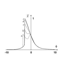
FIG. 1.: Bistability curves showing the intracavity intensity ${\cal I}=|{\cal A}|_{0}^{2}$ in the fundamental mode as a function of cavity detuning $\phi$ in the two mode approximation. The non-linear coefficient is $K=2.5$, the relative detuning $\delta\phi=\phi_{b}-\phi_{a}=0$. Differents curves in solid line correspond to increasing transverse mode order $p$: (a) $p=1$, (b) $p=2$, (c) $p=3$, (d) $p=4$, (e) $p=5$. The dashed line corresponds to the single mode approximation.

The modification of the bistability curve of the fundamental mode for various detunings between the two modes can be seen in figure 2, where the fundamental mode is coupled to the transverse mode $p=4$. Its perturbation is maximal when the transverse mode is resonant with the fundamental mode. Since the two modes experience both linear and non-linear phase shifts, resonance occurs for a non-zero linear detuning $\delta\phi=\phi_{b}-\phi_{a}$, where $\phi_{a}$ and $\phi_{b}$ denote respectively the linear phaseshifts of mode a and b.

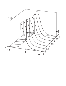
FIG. 2.: Intracavity intensity ${\cal I}=|{\cal A}|_{0}^{2}$ in the fundamental mode as a function of cavity detuning $\phi$ in the two mode approximation for a transverse mode $p=4$. The non-linear coefficient is $K=2.5$. Different curves correspond to different detunings $\delta\phi$ between the two modes. The dashed line marks the maxima of the bistability curves.

We will now analyze the influence of the non-linear coupling on fluctuations of the fundamental mode. It is first worth noting that the behaviour of coefficient $\lambda_{pp}$ for a large transverse mode order is

$$\lambda_{pp}=\frac{1}{4^{p}}\frac{\left(2p\right)!}{\left(p!\right)^{2}}\sim\sqrt{\frac{1}{p\pi}}.$$ (75)

This expression looks similar to a cross Kerr effect between the two modes. The value of this coefficient is decreasing only slowly with increasing mode order. The consequences will be discussed in the following paragraph.

The equation for the evolution of fluctuations in the two modes is obtained by linearizing the mean field equations (71,74). It is convenient to represent these fluctuations in a four element vector $\overrightarrow{\alpha}$

$$\overrightarrow{\alpha}=\left[\begin{array}[]{c}{\cal\alpha}\\ {\cal\alpha}^{*}\\ {\cal\beta}\\ {\cal\beta}^{*}\end{array}\right],$$ (76)

which satisfies the evolution equation:

$$\partial_{\tau}\overrightarrow{\alpha}=\overrightarrow{\alpha}^{{\rm in}}-\left(1+i\underline{\Phi}+iK\underline{M}\right)\overrightarrow{\alpha}.$$ (77)

$\underline{\Phi}$ is a diagonal four by four matrix containing the linear detunings $\phi_{a}$ and $\phi_{b}$ for the two modes. In the matrix $\underline{M}$ we have collected all non-linear terms. The exact expressions of both $\underline{\Phi}$ and $\underline{M}$ can be found in appendix (C). The input-output relations for field fluctuations in terms of correlation matrices $V_{{\rm out}}$ and $V_{{\rm in}}$ lead to the following relation between the correlation functions

$$\underline{V}^{{\rm out}}=\left(\frac{1-\underline{M}+i\omega}{1+\underline{M}-i\omega}\right)\underline{V}^{{\rm in}}\left(\frac{1-\underline{M}+i\omega}{1+\underline{M}-i\omega}\right)^{\dagger}.$$ (78)

Again the input field is supposed to be in the vacuum state. With the help of the exact expression for $\underline{M}$ (cf. equation (C3)) it is then possible to calculate the correlation functions of the output field. We will discuss the result by showing the corresponding numerical noise spectra.

Figure 3 shows the optimum noise reduction in the fundamental mode as a function of the dimensionless frequency $\omega$. We have supposed fluctuations to be measured in a homodyne detection[20, 21, 22] where the output beam is superimposed with a local oscillator whose spatial structure corresponds to the TEM₀₀ mode. The shot noise level is normalized to 0, perfect squeezing corresponds to $-1$. For all curves, the working point has been chosen on the upper branch of the bistability curve near the bistability turning point. Different curves correspond to transverse mode orders. Clearly, the effect of different non-linear coupling compared to the single mode approximation (dashed line) is a reduction and even suppression of the squeezing in the fundamental mode due to added

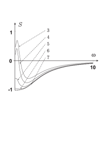
FIG. 3.: Optimum squeezing in the fundamental mode versus normalized frequency $\omega$ for a coupling to various higher order modes. The local oscillator is supposed to be matched to the TEM₀₀ mode. The working point is on the upper branch of the bistability curve close to the turning point. The non-linear coefficient is $K=2.5$, the relative detuning $\delta\phi=1$. Different curves in solid line correspond to increasing transverse mode order $p$ as mentioned in the figure. The dashed line corresponds to the single mode approximation.

noise coming from the perturbing mode, even though the spatial structure of the fundamental mode is perfectly matched to a cavity mode. It has to be noticed that this perturbation is higher than what would have been expected from the examination of the bistability curves: for the mode $p=5$, the steady state (figure 1(e)) is almost the steady state of the single mode cavity and only a small fraction of the incoming photons is transferred to the second mode. However, the added noise is sufficient to degrade significantly the squeezing around zero frequency. This large modification is due to the non negligible value of the ”cross Kerr” coupling $\lambda_{pp}$ between the two modes, which is still important for $p=5$.

The influence of the relative detuning between the two modes is shown in figure 4 where the squeezing spectra of the fundamental mode are plotted for a coupling with the transverse mode $p=4$ and various relative detunings. A comparison with figure 2 shows that fluctuations are much more sensitive to the detuning between the two modes than the mean field. In particular, quadrature squeezing in the fundamental mode is found to be completely suppressed in some range of cavity detuning. This shows that even in a perfectly matched cavity the non-linear transverse mode coupling can limit the value of quadrature squeezing attainable.

However, it is possible to recover an optimal quantum noise reduction in the output beam, if the spatial structure of the local oscillator is chosen more carefully. To illustrate this effect we have plotted in figure 5 the optimum squeezing in a field quadrature corresponding to a linear superposition between the fundamental and the pertubing mode. Fundamental and higher order mode are supposed to be resonant so that the perturbation due to the mode coupling is maximal. Even for a coupling with a mode of an order as low as $p=3$ the squeezing at

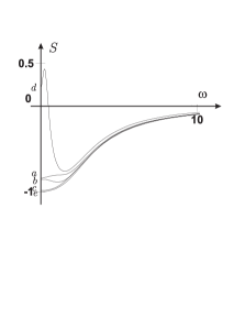
FIG. 4.: Optimum squeezing in the fundamental mode versus normalized frequency $\omega$ for various relative detunings $\delta\phi$. The working point is on the upper branch of the bistability curve close to the turning point. The non-linear coefficient is $K=2.5$. Different curves in solid line correspond to: (a) $\delta\phi=2$, (b) $\delta\phi=1$, (c) $\delta\phi=0$, (d) $\delta\phi=-1$, (e) $\delta\phi=-2$.

zero frequency is here almost perfect. This result has to be seen in comparison with figure 3 where we had shown the optimum squeezing in the output beam for the same experimental parameters but measured with a local oscillator the spatial structure of which was not optimized. It can also be noticed that here the noise reductions obtained for a coupling with different transverse modes show little differences. This can be understood from the squeezing mechanism. The bistability turning point is a critical point at which fluctuations in one of the field quadratures diverge. Since the system is lossless, fluctuations in the conjugated field quadrature have to tend to zero when the turning point is reached.

Compared to quadrature squeezing the influence of non-linear coupling on intensity squeezing is very differ-

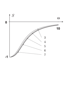
FIG. 5.: Optimum squeezing versus normalized frequency $\omega$ for a coupling to various higher order modes. The local oscillator is supposed to have an optimzed spatial structure. The working point is on the upper branch of the bistability curve close to the turning point. The non-linear coefficient is $K=2.5$, the relative detuning $\delta\phi=1$. Different curves in solid line correspond to increasing transverse mode order $p$ as mentioned in the figure. The single mode approximation coincides with the curve of mode 7.

ent. Figure 6 shows a comparison of the attainable intensity squeezing for a coupling to various modes. Clearly, this squeezing is very robust against the mode coupling. Furthermore the curves for various modes show little differences.

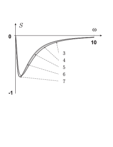
FIG. 6.: Intensity squeezing versus normalized frequency $\omega$ for a coupling to various higher order modes. The working point is on the upper branch of the bistability curve close to the turning point. The non-linear coefficient is $K=2.5$, the relative detuning $\delta\phi=1$. Different curves in solid line correspond to increasing transverse mode order $p$. The single mode approximation coincides with the curve $p=7$.

As expected from the squeezing by a lossless medium the noise at zero frequency is not modified since the total photon number is conserved. It also has to be noticed that for a coupling with mode $p=3$, the energy transfer from the fundamental mode to the transverse mode is not negligible. As a consequence the spatial structure of the beam going out of the cavity is quite different from the fundamental mode. Its intensity fluctuations are nevertheless reduced and this reduction corresponds to the one that could be expected from the single mode situation.

V Conclusion

In this paper, we have studied the non-linear coupling between transverse modes in a Kerr medium and its effect on bistability and quantum noise if the medium is placed inside a cavity. Whereas in free space the non-linear coupling becomes important as soon as the non-linear phase shift is appreciable, the use of an optical cavity can reduce significantly the perturbing effect of the transverse modes by selecting only a few modes. When fundamental and higher order modes belong to the same longitudinal mode family and only the fundamental mode is resonant, it is possible to treat higher order transverse modes perturbatively. The non-linear coupling leads to losses for the fundamental mode associated with an excess noise which contains a contribution from phase conjugated noise. The non-linear loss scales with the inverse of transverse mode spacing. Perturbations due to higher order transverse modes can therefore be neglected as soon as the transverse mode spacing becomes large compared to the cavity width. In this case a single mode approximation is valid.

In an experiment the fundamental mode may accidentally coincide with a transverse mode corresponding to a different longitudinal mode family. In this case, one can perform the calculations in a two mode approximation. We have shown that even if the spatial structure of the input beam is perfectly adapted to the fundamental mode of the cavity, the non-linear coupling produces an excess noise in the fluctuations of the fundamental mode and therefore can limit the optimum squeezing. The perturbation always arises when low order modes ($p\leq 6$) coincide resonantly with the fundamental mode during the resonance scan of the cavity. The reduction or even suppression of the obtainable squeezing occurs then in the central part of the noise spectrum. Quadrature squeezing in the fundamental mode is thus sensitive on perturbations by higher order modes. However, it is possible to recover the optimum squeezing in the output beam if the spatial structure of the local oscillator is optimized. Fluctuations are then not measured in the fundamental mode but in a mode corresponding to a linear superposition of the fundamental and the perturbing mode.

In contrast to quadrature squeezing quantum noise reduction in the total output intensity of the fundamental mode turns out to be very robust to perturbations by higher order modes. Hence, a Kerr medium inside an optical cavity remains a good intensity “noise eater” even when taking into account higher order transverse modes.

Acknowledgments: Thanks are due to S. Reynaud, C. Fabre, C. Schwob and L. Hilico for discussions.

A Nonlinear coupling coefficients

The calculation of expression for the non-linear coupling coefficients $\lambda_{pqrs}^{\left(lmno\right)}$ between Gauss-Laguerre modes in a Kerr medium can be performed by making use of the generating functions of the Laguerre Polynomials $G_{n}^{\left(l\right)}\left(x,z\right)$:

$$L_{n}^{\left(l\right)}\left(x\right) = \frac{1}{n!}\left.\frac{\partial^{n}}{\partial z^{n}}\right|_{z=0}$$ (A1)

$$G_{n}^{\left(l\right)}\left(x,z\right) = \frac{1}{\left(1-z\right)^{l+1}}\exp\left(\frac{xz}{z-1}\right).$$ (A2)

The coupling coefficient may then be reexpressed as a function of the generating functions

$$\lambda_{pqrs}^{\left(lmno\right)} = \frac{2}{p!q!r!s!}\frac{\partial^{p+q+r+s}}{\partial z_{1}^{p}\partial z_{2}^{q}\partial z_{3}^{r}\partial z_{4}^{s}}\int_{0}^{\infty}dxx^{l+m}G_{p}^{\left(l\right)}\left(x,z_{1}\right)$$ (A5)

$$\times G_{q}^{\left(l\right)}\left(x,z_{2}\right)G_{r}^{\left(l\right)}\left(x,z_{3}\right)G_{s}^{\left(l\right)}\left(x,z_{4}\right)$$

$$\times\exp\left[-2x\right]\left.\right|_{z_{1}=z_{2}=z_{3}=z_{4}=0}.$$

In cylindrical symmetry and with $r=s=0$ they simplify to

$$\lambda_{pq=} = \frac{2}{p!q!}\frac{\partial^{p+q}}{\partial z_{1}^{p}\partial z_{2}^{q}}\int_{0}^{\infty}dx\frac{1}{\left(1-z_{1}\right)\left(1-z_{2}\right)^{1}}$$ (A7)

$$\times\exp x\left(\frac{z_{1}}{z_{1}-1}+\frac{z_{2}}{z_{2}-1}-2\right)\left.\right|_{z_{1}=z_{2}=0}$$

$$= \frac{2}{p!q!}\frac{\partial^{p+q}}{\partial z_{1}^{p}\partial z_{1}^{q}}\frac{1}{2-z_{1}-z_{2}}\left.\right|_{z_{1}=z_{2}=0}=\frac{1}{2^{p+q}}\frac{\left(p+q\right)!}{p!q!}$$ (A8)

B The multimode approximation

The evolution equation of mode p may be rewritten as

$$\overrightarrow{\alpha}_{p}=\underline{G}_{p}\overrightarrow{\alpha}_{p}^{{\rm in}}+i\underline{G}_{p}\underline{\eta}\underline{M}_{p0}\overrightarrow{\alpha}_{0}+i\underline{G}_{p}\underline{\eta}\sum_{q\neq p,0}\underline{M}_{pq}\overrightarrow{\alpha}_{q}.$$ (B1)

By iterating once and inserting the result in the evolution equation of the fundamental mode (B1) gives

$$\underline{G}_{0}^{-1}\overrightarrow{\alpha}_{0} = \overrightarrow{\alpha}_{0}^{{\rm in}}-\sum_{q\neq 0}\underline{\eta}\underline{M}_{0q}\underline{G}_{q}\underline{\eta}\underline{M}_{q0}\overrightarrow{\alpha}_{0}$$ (B2)

$$- i\sum_{q\neq 0}\sum_{r\neq q,r\neq 0}\underline{\eta}\underline{M}_{0q}\underline{G}_{q}\underline{\eta}\underline{M}_{qr}\underline{G}_{r}\underline{\eta}\underline{M}_{r0}\overrightarrow{\alpha}_{0}$$ (B5)

$$+i\underline{\eta}\sum_{q\neq 0}\underline{M}_{0q}\underline{G}_{q}\overrightarrow{\alpha}_{q}^{{\rm in}}$$

$$-\sum_{q\neq 0}\sum_{r\neq q,0}\underline{\eta}\underline{M}_{0q}\underline{G}_{q}\underline{\eta}\underline{M}_{qr}\underline{G}_{r}\overrightarrow{\alpha}_{r}^{{\rm in}}.$$

This equation may be resolved for $\alpha_{0}$, and fluctuations in the fundamental mode may now be rewritten in the more convenient form

$$\overrightarrow{\alpha}_{0}=\underline{\tilde{G}}_{0}\left(\overrightarrow{\alpha}_{0}^{{\rm in}}+i\underline{\eta}\sum_{q\neq 0}\underline{\tilde{T}}_{q}\overrightarrow{\alpha}_{q}^{{\rm in}}\right),$$ (B6)

with the propagator $[\tilde{G}_{0}]$ for the fundamental mode and the transfer matrix $\underline{\tilde{T}}_{q}$

$$\underline{\tilde{G}}_{0} = \left(1-i\omega+\underline{R}_{0}+i\underline{\eta}\phi_{0}\right)^{-1},$$ (B7)

$$\underline{\tilde{T}}_{q} = \underline{M}_{0q}\underline{G}_{q}+i\sum_{r\neq q,0}\underline{M}_{0q}\underline{G}_{q}\underline{\eta}\underline{M}_{qr}\underline{G}_{r},$$ (B8)

$$\underline{R}_{0} = -i\underline{\eta}\underline{M}_{00}+\sum_{q\neq 0}\underline{\eta}\underline{M}_{0q}\underline{G}_{q}\underline{\eta}\underline{M}_{q0}$$ (B9)

$$+ i\sum_{q\neq 0}\sum_{r\neq q,0}b\underline{\eta}\underline{M}_{0q}\underline{G}_{q}\underline{\eta}\underline{M}_{qr}\underline{G}_{r}\underline{\eta}\underline{M}_{r0}.$$ (B10)

In the multimode perturbative expansion the expression of $\underline{R}_{0}$ can be simplified to

$$\underline{R}_{0} = +\mu_{2}\frac{K^{2}{\cal A}_{0}^{2}}{\phi_{{\rm T}}^{2}}\left(\begin{array}[]{cc}3\left|{\cal A}_{0}\right|^{2}&2{\cal A}_{0}^{2}\\ 2{\cal A}_{0}^{*2}&3\left|{\cal A}_{0}\right|^{2}\end{array}\right)-3i\mu_{2}\frac{\omega K^{2}{\cal A}_{0}^{4}}{\phi_{{\rm T}}^{2}}$$ (B22)

$$-iK\left(\begin{array}[]{cc}2\left|{\cal A}_{0}\right|^{2}&{\cal A}_{0}^{2}\\ -{\cal A}_{0}^{*2}&-2\left|{\cal A}_{0}\right|^{2}\end{array}\right)-3i\frac{K^{2}{\cal A}_{0}^{2}}{\phi_{{\rm T}}}\left(\mu_{1}-\mu_{2}\frac{\phi_{0}}{\phi_{{\rm T}}}\right)$$

$$\times\left(\begin{array}[]{cc}3\left|{\cal A}_{0}\right|^{2}&2{\cal A}_{0}^{2}\\ -2{\cal A}_{0}^{*2}&-3\left|{\cal A}_{0}\right|^{2}\end{array}\right)$$

$$-12i\mu_{3}\frac{K^{3}{\cal A}_{0}^{4}}{\phi_{{\rm T}}^{2}}\left(\begin{array}[]{cc}4\left|{\cal A}_{0}\right|^{2}&3{\cal A}_{0}^{2}\\ -3{\cal A}_{0}^{*2}&-4\left|{\cal A}_{0}\right|^{2}\end{array}\right).$$

The specific expression for the transfer matrix evaluates to

$$\underline{\tilde{T}}_{q} = \left(-\frac{i\lambda_{q}K}{q\phi_{T}}+i\frac{\lambda_{q}\phi_{0}K}{q^{2}\phi_{T}^{2}}-2i\frac{K^{2}{\cal I}_{0}}{\phi_{T}^{2}}\sum_{r\neq 0}\frac{\lambda_{r}\lambda_{qr}}{qr}\right)$$ (B32)

$$\times\left(\begin{array}[]{cc}2\left|{\cal A}_{0}\right|^{2}&{\cal A}_{0}^{2}\\ -{\cal A}_{0}^{*2}&-2\left|{\cal A}_{0}\right|^{2}\end{array}\right)$$

$$-i\frac{K^{2}}{\phi_{T}^{2}}\sum_{r\neq 0}\frac{\lambda_{q}\lambda_{qr}}{qr}\left(\begin{array}[]{cc}5\left|{\cal A}_{0}\right|^{2}&4{\cal A}_{0}^{2}\\ -4{\cal A}_{0}^{*2}&-5\left|{\cal A}_{0}\right|^{2}\end{array}\right)$$

$$+\frac{\lambda_{q}K}{q^{2}\phi_{T}^{2}}\left(1-i\omega\right)\left(\begin{array}[]{cc}2\left|{\cal A}_{0}\right|^{2}&{\cal A}_{0}^{2}\\ {\cal A}_{0}^{*2}&2\left|{\cal A}_{0}\right|^{2}\end{array}\right).$$

C The two mode approximation

The evolution equation for the complex amplitude of the two modes is

$$\partial_{\tau}\overrightarrow{\alpha}=\overrightarrow{\alpha}^{{\rm in}}-\left(1+i\underline{\Phi}+iK\underline{M}\right)\overrightarrow{\alpha},$$ (C1)

with the four dimensional matrices $[\phi]$ and $[M]$:

$$\begin{array}[]{ccc}\underline{\Phi}=\left[\begin{array}[]{cc}\Phi_{a}&0\\ 0&\Phi_{b}\end{array}\right],&\Phi_{a}=\left[\begin{array}[]{cc}\phi_{a}&0\\ 0&-\phi_{a}\end{array}\right],&\Phi_{b}=\left[\begin{array}[]{cc}\phi_{b}&0\\ 0&-\phi_{b}\end{array}\right],\end{array}$$ (C2)

$$\underline{M}=\underline{M}_{0}+\lambda_{p}\underline{M}_{1}+\lambda_{pp}\underline{M}_{2}+\lambda_{ppp0}\underline{M}_{3}+\lambda_{pppp}\underline{M}_{4},$$ (C3)

$$\begin{array}[]{cc}M_{a}=\left[\begin{array}[]{cc}-2\left|{\cal A}\right|^{2}&-{\cal A}^{2}\\ {\cal A}^{*2}&2\left|{\cal A}\right|^{2}\end{array}\right],&M_{b}=\left[\begin{array}[]{cc}-2\left|{\cal B}\right|^{2}&-{\cal B}^{2}\\ {\cal B}^{*2}&2\left|{\cal B}\right|^{2}\end{array}\right]\end{array}$$ (C9)

$$\begin{array}[]{cc}M_{ab}=\left[\begin{array}[]{cc}-2\left({\cal A^{*}B+AB^{*}}\right)&-2{\cal AB}\\ 2{\cal AB}&2\left({\cal A^{*}B+AB^{*}}\right)\end{array}\right]&\end{array}$$ (C13)

$$\begin{array}[]{cc}\underline{M}_{0}=\left[\begin{array}[]{cc}M_{a}&0\\ 0&0\end{array}\right],&\underline{M}_{1}=\left[\begin{array}[]{cc}M_{ab}&M_{a}\\ M_{a}&0\end{array}\right],\\[14.22636pt] \underline{M}_{2}=\left[\begin{array}[]{cc}M_{b}&M_{ab}\\ M_{ab}&M_{a}\end{array}\right],&\underline{M}_{3}=\left[\begin{array}[]{cc}0&M_{b}\\ M_{b}&M_{ab}\end{array}\right],\\[14.22636pt] \underline{M}_{4}=\left[\begin{array}[]{cc}0&0\\ 0&M_{b}\end{array}\right].\end{array}$$ (C14)

REFERENCES

- [1] L. A. Lugiato and G. Strini, Opt. Comm. 41, 67 (1982)
- [2] M. Xiao, H. J. Kimble, and H. J. Carmichael, J. Opt. Soc. Am. B4, 1546 (1987)
- [3] M. A. Reid, Phys. Rev. A37, 4792 (1988)
- [4] L. Hilico, C. Fabre, S. Reynaud. and E. Giacobino, Phys. Rev. A46, 4397 (1992)
- [5] M. J. Collett and D. F. Walls, Phys. Rev. A32, 2887 (1985)
- [6] R. M. Shelby, M. D. Levenson, D. F. Walls, A. Aspect, and G. J. Milburn, Phys. Rev. A33, 4008 (1986)
- [7] S. Reynaud, C. Fabre, E. Giacobino, and A. Heidmann, Phys. Rev. A40, 1440 (1989)
- [8] M. G. Raizen, L. A. Orozco, M. Xiao, T. L. Boyd, and H. J. Kimble, Phys. Rev. Lett. 59, 198 (1987)
- [9] D. M. Hope, H. A. Bachor, P. J. Manson, D. E. McClelland, P. T. H. Fisk, Phys. Rev. A46, R1181 (1992)
- [10] A. Lambrecht, J. M. Courty, S. Reynaud, E. Giacobino, Appl. Phys. B60, 129 (1995)
- [11] P. D. Drummond, IEEE J. Quant. Electr. QE17, 301 (1981)
- [12] M. Xiao, H. J. Kimble, and H. J. Carmichael, Phys. Rev. A35, 3832 (1987)
- [13] D. M. Hope, D. E. McClelland, and C. M. Savage, Phys. Rev. A41, 5074 (1990)
- [14] A. Lambrecht, J. M. Courty, and S. Reynaud, Journal de Physique II (to be published)
- [15] L. A. Lugiato and L. M. Narducci, Les Houches Lecture Notes, Session LIII, 1990, eds. J. Dalibard, J. M. Raimond and J. Zinn-Justin, Elsevier Science Publisher
- [16] L. A. Lugiato, A. Gatti and H. Wiedemann, Les Houches Lecture Notes, Session LXIII, 1995, eds. S. Reynaud, E. Giacobino and J. Zinn-Justin, Elsevier Science Publisher (to appear) and references therein
- [17] S. Reynaud and A. Heidmann, Opt. Comm. 71, 209 (1989)
- [18] M. Abramovitz and I. A. Stegun, Handbook of Mathematical Functions, Dover Publications, New York, 1972
- [19] J. M. Courty, P. Grangier, L. Hilico and S. Reynaud, Opt. Comm. 83, 251 (1991)
- [20] C. M. Caves, Phys. Rev. D23, 1693 (1981)
- [21] H. P. Yuen and V. W. S. Chan, Opt. Lett. 8, 177 (1983)
- [22] J. H. Shapiro and S. S. Wagner, IEEE J. Quant. Electr. QE20, 803 (1984)