The Born and Markov approximations for atom lasers.

Abstract

We discuss the use of the Born and Markov approximations in describing the dynamics of an atom laser. In particular, we investigate the applicability of the quantum optical Born-Markov master equation for describing output coupling. We derive conditions based on the atomic reservoir, and atom dispersion relations for when the Born-Markov approximations are valid and discuss parameter regimes where these approximations fail in our atom laser model. Differences between the standard optical laser model and the atom laser are due to a combination of factors, including the parameter regimes in which a typical atom laser would operate, the different reservoir state which is appropriate for atoms, and the different dispersion relations between atoms and photons. We present results based on an exact method in the regimes in which the Born-Markov approximation fails. The exact solutions in some experimentally relavent parameter regimes give non-exponential loss of atoms from a cavity.

I Introduction

An atom laser is a device which, in analogy to the optical laser, would emit a coherent beam of bosonic atoms. Various models of atom lasers have been presented [2, 3, 4, 5, 6, 7, 8, 9].

Many of these schemes are based around a master equation description for the dynamics of the system[2, 3, 4, 5, 9]. In these, the atom laser output is described by a Born-Markov master equation. Making the Born-Markov approximation involves assuming that reservoir correlations decay rapidly compared with the system damping time and that the reservoir does not change significantly with time due to the effect of the system. We discuss these approximations in the context of atom output coupling.

Born-Markov master equations were initially derived for optical systems[10]. There they are used to describe a system (for instance an optical laser mode) coupled to a large, unchanging reservoir (the external modes). In optics the Born-Markov approximations allow an equation containing only system variables to be derived. One of the fundamental assumptions involved in deriving such a Born-Markov master equation is that the reservoir correlation functions decay rapidly. This allows the reservoir to be approximated as unchanging in time. While it is assumed the system does not affect the reservoir, the reservoir does affect the system.

An equation in terms of system variables alone is also an important goal for describing atom lasers. However, atom and photon devices work in substantially different parameter regimes. Moreover, atoms and photons have different dispersion relations, which affects the behaviour of the reservoir correlation functions. Furthermore, typically the reservoir for an optical cavity is taken to be at thermal equilibrium at a nonzero temperature. For atoms, a vacuum reservoir with all modes initially empty is often more appropriate.

In this paper we look at the validity of the Born-Markov master equation for describing output coupling from a single mode atomic system to a reservoir. The reservoir is described as a continuum of free-space modes. Our description of the coupling will initially be quite general, though our later discussion will focus on particular schemes in which the atom becomes free of the system through a change of state. Such a change of state to an untrapped state can be achieved using either a Raman transition [8] or an RF transition[12, 13, 14]. We will also discuss the effects of gravity on output coupling. In the latter part of the paper we will focus on broadband coupling. This allows a comparison with exact results[16, 17], however we also present finite coupling results which more accurately describe output coupling through a change of state. We will discuss exact equations which can be obtained in regimes where the Born-Markov approximations fail.

In section II we present our model of output coupling from a single mode trap. This allows exact equations of motion, and their solutions, to be obtained for system variables. In section III we model this system using the master equation formalism, emphasising the importance of the Born and Markov approximations. In section IV we then consider the validity of these approximations. In the optical case, the adequacy of the Born-Markov approximation means that the standard model we are using leads to exponential decay of the number of photons in a cavity. The equivalent model for atoms does not lead to an atom number which tends to zero for sufficiently long time. In section VI we discuss the reasons for this and consider the results obtained from models which include the effects of gravity. Having noted that the Born-Markov approximations may fail, we discuss in section VII a non-Markovian master equation and show that for atoms the Born-approximation is not valid for our parameters even if we avoid making the Markov approximation. In the regimes where these approximations fail, the output field becomes correlated with the system and hence cannot be traced over to provide a master equation. Finally we discuss ways of proceeding when the Born-Markov master equation fails. The most straightforward method is that used in section II where exact equations for the whole system and reservoir are obtained.

II Exact solutions

Dilute gas Bose Einstein Condensates (BEC) are now available in the laboratory. To produce a continuously running atom laser from a BEC requires the addition of a suitable pumping mechanism, and an output coupler. A change of atomic state through RF transition has been used to produce a “pulsed atom laser”[12, 13]. The output coupling from a single mode to a large reservoir is sometimes described by a Born-Markov master equation of the form

$$\frac{d\rho(t)}{dt} = C(2a\rho(t)a^{{\dagger}}-a^{{\dagger}}a\rho(t)-\rho(t)a^{{\dagger}}a),$$ (1)

where $C$ describes the strength of the coupling and $a$ ($a^{{\dagger}}$) is the annihilation (creation) operator for the single mode system. Two important approximations involved in such a description are that the evolution is Markovian and that it depends only on the system operators. The Markovian property means that the rate of change of the state depends only on the state at that time. There is no explicit dependence on the state at previous times. The equation is a function of system variables only, due to tracing over the reservoir. This is appropriate if the reservoir remains uncorrelated with the system. In fact, it is approximated in deriving Eq. (1) that the reservoir does not change with time.

We wish to investigate these two approximations, and their validity for describing atomic output coupling. In a full atom laser model it is essential that a pumping term is also included. However, in this paper we consider a single mode coupled only through output coupling to the outside world. Experimentally this corresponds to a leaky BEC. We focus on the output coupling term which would be present in a full master equation model alongside other terms.

We begin by considering a generic output coupling mechanism which we have previously analysed in the context of Heisenberg equations of motion[16, 17]. Here we investigate how such a model can be described by a density operator equation - in particular a master equation. When the output field is constrained by a waveguide such as in a hollow optical fibre model[8], the output field is effectively one dimensional. We consider a single mode system (the lasing mode with creation operators $a^{{\dagger}}$) coupled to a one-dimensional continuum of free space modes. The free space modes are labelled by their momentum, $\hbar k$ (creation operators $b_{k}^{{\dagger}}$). In a general three dimensional model $b_{k}$ would also be labelled by indicies describing the transverse modes. Here, however, we suppress these indicies and assume that the output is coupled into a waveguide with the atoms remaining in a single transverse mode. The Hamiltonian describing the system is given by

$${H} = {H_{\mbox{s}}}+{H_{\mbox{r}}}+{H_{\mbox{sr}}},$$ (2)

$${H_{\mbox{s}}} = \hbar\omega_{0}~{}a^{{\dagger}}a,$$ (3)

$${H_{\mbox{r}}} = \int_{-\infty}^{\infty}\mbox{dk}~{}\hbar\omega_{k}~{}b_{k}^{{\dagger}}b_{k},$$ (4)

$${H_{\mbox{sr}}} = -i\hbar\int_{-\infty}^{\infty}\mbox{dk}~{}~{}(\kappa(k)~{}b_{k}a^{{\dagger}}-\kappa^{*}(k)~{}b_{k}^{{\dagger}}a).$$ (5)

The function $\kappa(k)$ describes the shape of the coupling in $k$ space, and is left general here. By appropriately choosing $\kappa(k)$ we may simulate a wide range of practical output coupling mechanisms, including position dependant coupling and the effect of momentum kicks. The latter may result from laser photons when an atom undergoes a change of state. Choosing $\kappa(k)$ as constant over a broad region corresponds to broadband coupling. This model is used for optical input-output theory[11], and in proposed atom laser theories which result in Born-Markov master equations. For the atom case this model ignores potentially important effects such as gravity and atom-atom interactions. For now, we neglect these effects in order to investigate the validity of the Born-Markov approximations. We use this model to understand the differences between optical and atomic output coupling. We will extend the model in section VI.

We use the Hamiltonian presented above to write Heisenberg equations of motion for the operators $a$, $b_{k}$. We can also obtain equations for combinations of these operators which may be of more interest, such as the number of atoms in the system, $a^{{\dagger}}a$. These equations can be difficult to solve in general. However, since they include the output and system explicitly, they describe the dynamics of the model exactly[16, 17]. Exact solutions can be compared with Born-Markov master equations.

To facilitate this comparison we present exact equations for the expectation values of the system operators, $a^{{\dagger}}$ and $a^{{\dagger}}a$. In these we assume (as we will do in the master equation descriptions to follow) that the reservoir is initially empty, $\langle b_{k}^{{\dagger}}(0)b_{k}(0)\rangle=0$. We do not place any further restrictions on $\langle b_{k}^{{\dagger}}(t)b_{k}(t)\rangle$. This is the first fundamental difference between the atom and photon case. An empty reservoir for photons is inapropriate at finite temperatures[18]. In experiments where a Bose-Einstein condensate is allowed to leak out of a trap, however, the most appropriate initial state for the outside atom modes is a vacuum. Similarly, for an atom laser in a hollow fibre, which we discussed in [8], the initial output modes would be empty.

We obtain

$$\frac{d}{dt}\langle a^{{\dagger}}(t)\rangle = i\omega_{0}\langle a^{{\dagger}}(t)\rangle-$$ (7)

$$~{}\int_{0}^{t}d\tau~{}f^{\prime*}(\tau)\langle a^{{\dagger}}(t-\tau)\rangle e^{i\omega_{0}\tau},$$

$$\frac{d}{dt}\langle a^{{\dagger}}(t)a(t)\rangle = -\int_{0}^{t}d\tau~{}f^{\prime}(\tau)~{}\langle a^{{\dagger}}(t)a(t-\tau)\rangle e^{-i\omega_{0}\tau}~{}$$ (9)

$$~{}+\mbox{h.c}.$$

These equations have solutions given by [16, 17]

$$\langle a^{{\dagger}}(t)\rangle = \langle a^{{\dagger}}(0)\rangle e^{i\omega_{0}t}~{}{\cal L}^{-1}\left\{\frac{1}{s+{\cal L}\left\{f^{\prime}(t)^{*}\right\}(s)}\right\}(t),$$ (10)

$$\langle a^{{\dagger}}(t)a(t)\rangle = \langle a^{{\dagger}}(0)a(0)\rangle~{}\times$$ (12)

$$~{}\left|{\cal L}^{-1}\left\{\frac{1}{s+{\cal L}\left\{f^{\prime}(t)\right\}(s)}\right\}(t)\right|^{2},$$

where ${\cal L}$ and ${\cal L}^{-1}$ denote Laplace and inverse Laplace transforms respectively. $f^{\prime}(t)$ is the function defined by [17]

$$f^{\prime}(t) = \int_{-\infty}^{\infty}dk|\kappa(k)|^{2}e^{-i(\omega_{k}-\omega_{0})t}.$$ (13)

The function $f(t)=f^{\prime}(t)e^{-i\omega_{0}t}$ is the “reservoir correlation function” in the master equation picture which we describe in the next section. Here $\omega_{k}=\hbar k^{2}/(2m)$ for atoms, in contrast to $\omega_{k}=c_{L}|k|$ for photons. Here $m$ is the mass of the atoms, and $c_{L}$ is the speed of light.

For a previously described output coupling from a condensate through state change[17], $\kappa(k)$ is a Gaussian of width $\sigma_{k}$,

$$\kappa(k) = i\Gamma^{\frac{1}{2}}(2\pi\sigma_{k}^{2})^{-1/4}\exp{\left(-k^{2}/(4\sigma_{k}^{2})\right)}.$$ (14)

Here, the strength of the coupling is given by the coupling constant, $\Gamma$. For this form of coupling $f^{\prime}(t)$ may be evaluated as:

$$f^{\prime}(\tau)=\frac{e^{i\omega_{0}\tau}\Gamma}{\sqrt{1+i\alpha\tau}},$$ (15)

where we have defined

$$\alpha=\hbar\sigma_{k}^{2}/m.$$ (16)

For the broadband limit of Eq. (16) (discussed in section IV) we may use methods similar to those given in reference [17] to obtain an analytical form for the inverse Laplace transform,

$${\cal L}^{-1}\left\{\frac{1}{s+{\cal L}\left\{f^{\prime}(t)\right\}(s)}\right\}(t) = e^{i\omega_{0}t}$$ (18)

$$\rule{-99.58464pt}{0.0pt}\times~{}(W(a,b,c)+W(b,a,c)+W(c,b,a)),$$

$$W(a,b,c) = \frac{a^{2}e^{a^{2}t}~{}(1+\mbox{erf}[a\sqrt{t}])}{(a-b)(a-c)}.$$ (19)

The variables, a,b and c are the three solutions of the equation $s^{3}+i\omega_{0}s+\Gamma c\sqrt{i}=0$. Note that Eq. (10) gives that $\langle a(t)\rangle$ will always remain zero if $\langle a(0)\rangle=0$. For the case of damping of a BEC which we consider here, the initial state corresponds to a BEC in an atom trap. According to spontaneous symmetry breaking arguments BECs are in coherent states with a definite global phase [15], so that $\langle a(0)\rangle\neq 0$. This is a useful assumption. Nevertheless, even if $\langle a\rangle=0$, the form of the equation for $\langle a(t)\rangle$ must be as given.

The equations of motion given by Eqs. (7,9) and the corresponding solutions, Eqs. (10,12) are exact for the system under consideration. In specific cases it is very difficult to solve for these inverse Laplace transforms. Moreover, the Heisenberg equations for system operators depend on the external operators, $b_{k}(0)$ in general. We next investigate equations of motion based on the Born and Markov approximations. These are compared with the exact solutions given above.

III The Born-Markov Master Equation

Derivations of the Born-Markov master equation for a general system reservoir interaction are given in references [18, 19, 20]. Here we present a derivation for the specific model of Eq. (2) to Eq.(5). We assume that the atom reservoir is initially in a vacuum state - that is, there are initially no atoms outside the system. This assumption was also made in the exact solutions presented in Sec. II. We make the Born approximation. It involves ignoring correlations which may arise between the system and reservoir and ignoring any time evolution of the reservoir density operator. We use the interaction Hamiltonian in Eq. (5). This leads to the non-Markovian master equation:

$$\frac{d{\widetilde{\rho}}}{dt} = -\int_{0}^{t}~{}d\tau\left\{a^{{\dagger}}a\widetilde{\rho}(t-\tau)-a\widetilde{\rho}(t-\tau)a^{{\dagger}}\right\}\times$$ (21)

$$f^{\prime}(\tau)~{}+\mbox{h.c},$$

where, ${\widetilde{\rho}}$ is the density operator in the interaction picture. The function, $f^{\prime}(\tau)$, defined as $f^{\prime}(\tau)=f(\tau)~{}e^{i\omega_{0}\tau}$ is the same as defined in Eq. (13) and Eq. (15). Here $f(\tau)$ is the reservoir correlation function.

Eq. (21) is non-Markovian. The second major approximation required to produce a Born-Markov master equation is the Markov approximation. The Markov approximation is made on the assumption that the reservoir correlation function, $f(\tau)$ goes to zero rapidly compared with the time scale on which $\widetilde{\rho}(t)$ changes. Making the Markov approximation thus involves replacing the terms $\widetilde{\rho}(t-\tau)$ in Eq. (21) with $\widetilde{\rho}(t)$. In the optics case, this approximation is also usually accompanied with the extension of the upper limit of the integral from $t$ to infinity. Making these approximations gives

$$\dot{\widetilde{\rho}} = \left\{(c+c^{*})a\widetilde{\rho}(t)a^{{\dagger}}-c~{}a^{{\dagger}}a\widetilde{\rho}(t)-c^{*}\widetilde{\rho}(t)a^{{\dagger}}a\right\},$$ (22)

where

$$c = \int_{0}^{t\rightarrow\infty}d\tau\int_{-\infty}^{\infty}|\kappa(k)|^{2}e^{-i(\omega_{k}-\omega_{0})\tau}dk$$ (23)

$$= \int_{0}^{\infty}f^{\prime}(\tau)d\tau$$ (24)

$$= \frac{\Gamma\sqrt{2\pi}\exp{\left[-\omega_{0}/\alpha\right]}}{\sqrt{2\omega_{0}\alpha}}~{}\left(1+\mbox{Erf}\left[i\sqrt{\frac{\omega_{0}}{\alpha}}\right]\right).$$ (25)

The upper integration limit $t$ has been extended to $\infty$, as is done in the optical case, without affecting our subsequent conclusion regarding the Born and Markov approximations. This produces an equation of the form which has been used previously to describe atom lasers. We further note that we could redefine $c$ to be real without loss of generality by incorporating the imaginary part of $c$ in with the free part of the system Hamiltonian. This reduces the form of the loss term to the familiar $C(2a\rho a^{{\dagger}}-a^{{\dagger}}a\rho-\rho a^{{\dagger}}a)$, with $C={\cal R}e[c]$ the (real) coupling strength.

The value of the constant $c$ depends on the form of $f^{\prime}(\tau)$. In the following, we consider $f^{\prime}(t)$ to be either that resulting from the Gaussian coupling presented in this section, or the broadband limit of this function which we discuss in the next section.

IV Timescale conditions

The Born-Markov master equation, Eq. (22), is the form used recently in various discussions of atom laser dynamics [2, 3, 4, 5, 9]. This Born-Markov master equation is used ubiquitously in quantum optics. The validity of the Markov approximation depends on the interplay between the reservoir correlation timescale, the system timescale, and the timescale on which the system decays.

The condition for the validity of the Born-Markov approximations is given in standard optics texts by the timescale separation condition [18, 19, 20]

$$t_{R}<<\Delta t<<t_{D}$$ (26)

where $t_{R}$ is the reservoir correlation time, and $t_{D}$ is the cavity decay time. $\Delta t$ defines a coarse grained timescale on which the equations of motion are valid. Generally $t_{R}$ is defined as the “timescale on which the reservoir correlations are non-zero”. $t_{D}$ is the decay timescale of the system which can be obtained by solving the equations for system and reservoir self consistently. In the Markov approximation this timescale goes as $1/(c+c^{*})$ for $c$ similar to that defined in Eq. (25) except with the optics dispersion relation.

Both $t_{R}$ and $t_{D}$ depend on the function $f^{\prime}(\tau)$, and thus in turn on the form of $\omega_{k}$ as a function of $k$. For atoms $\omega_{k}=\hbar k^{2}/(2m)$, whereas for photons $\omega_{k}=c_{L}|k|$, where $c_{L}$ is the speed of light. It also depends on factors such as the nature of the reservoir and the parameter regime in which atom lasers operate.

A second timescale condition for the Born-Markov approximation which is discussed in some treatements [19, 20] of the optical Born-Markov approximation is that the system timescale, defined as $t_{s}=1/\omega_{0}$ must satisfy

$$t_{s}<<\Delta t.$$ (27)

This is equivalent to requiring $\omega_{0}$ to be very large. A large $\omega_{0}$ condition is required in optics for a number of reasons. First, the initial coupling Hamiltonian, of the form ($ab_{k}^{{\dagger}}+a^{{\dagger}}b_{k})$, is in the rotating wave approximation and ignores terms of the form $ab_{k}$ and $a^{{\dagger}}b_{k}^{{\dagger}}$. This rotating wave approximation in optics can only be made in the case of large $\omega_{0}$. For the atom coupling, however, the correct form of the coupling does not include such (non atom number conserving) terms, even for small $\omega_{0}$. The terms which are eliminated in the optics case[19, 20] through the assumption of large $\omega_{0}$ are already zero for our model, due to the assumption of an atom vacuum reservoir. Thus, one may be led from these treatments to suppose that the Born-Markov approximation is made independently of $\omega_{0}$ for an atom-vacuum reservoir. This however is not the case as we will discuss later.

In optics, these timescale conditions are usually satisfied. For a coupling based on a mirror it is standard to assume that the coupling is broadband[10]. That is, we assume $\kappa(k)$ is flat in k-space. In this case the reservoir correlation function, $f^{\prime}(\tau)$, given by Eq. (13) becomes

$$f^{\prime}(\tau) \approx |\kappa(k_{0})|^{2}e^{i\omega_{0}\tau}~{}\int_{-\infty}^{\infty}~{}e^{-i\omega_{k}\tau}~{}dk$$ (28)

$$= 2|\kappa(k_{0})|^{2}~{}\int_{-\omega_{0}/c_{L}}^{\infty}~{}e^{-ic_{L}k\tau}~{}dk$$ (29)

$$\approx 2|\kappa(k_{0})|^{2}~{}\delta(\tau).$$ (30)

In the final equation the Dirac delta function, $\delta(\tau)$, is obtained by extending the frequency integral into physically unrealistic negative frequencies. This is a standard technique in optics [10] where $\omega_{0}$ is typically large.

Typically, for a laser, $\omega_{0}\approx 10^{15}\mbox{s}^{-1}$ is large and the assumption of a Dirac delta function decay is very good. Atom traps work in rather different parameter regimes with $\omega_{0}\approx 10^{3}\mbox{s}^{-1}$. If we avoid using negative frequencies, with the assumption of the empty reservoir considered here, we obtain the sum of a Dirac delta function, and an imaginary part corresponding to the Cauchy principal value of the integral in Eq. (30).

$$f^{\prime}(\tau)=\frac{2\pi}{c_{L}}|\kappa(k_{0})|^{2}e^{i\omega_{0}\tau}\left(\delta(\tau)-\frac{i}{\pi\tau}\right).$$ (31)

However, for an optical reservoir this estimate of correlation function decay based on our reservoir model is not strictly valid. This is because, while we have considered here the photonic dispersion relation, a vacuum is unrealistic for an optical reservoir at finite temperatures. More appropriate is a thermal reservoir, which leads to a decay time of order $\hbar/k_{B}T\approx 10^{-13}\mbox{s}$[18].

These reservoir correlation times must be short compared with the decay time, $t_{D}$. The system timescale, $1/\omega_{0}$ must also be short compared with $t_{D}$ for a standard optical reservoir. $t_{D}$ is the timescale of exponential decay, given by $e^{-(c+c^{*})t}$ in the Born-Markov limit. From an equivalent derivation of the optical master equation to that given in section III, the decay timescale is given by $t_{D}=1/(c+c^{*})\propto(\sigma_{k}/\Gamma)$. That is $t_{D}$ is inversely proportional to the strength of the coupling, given by $\Gamma/\sigma_{k}$ in the broadband limit. We will see later that for the atom coupling, the different dispersion relation makes $t_{D}$ depend on $\omega_{0}$ and other parameters, such as the mass of the atom. For optical systems this decay time is typically of the order $10^{-8}\mbox{s}$. Thus, in typical optical systems, the Born-Markov approximation holds for a number of reasons. The condition $t_{R}<<t_{D}$ holds, because in the large $\omega_{0}$ limit the reservoir correlations decay as a Dirac delta function. $t_{D}$ does not depend on $\omega_{0}$ and is typically many orders of magnitude larger than the reservoir decay times. Similarly, the system timescale $t_{s}$ for realistic optical cavities is very much shorter than the decay timescale, $t_{D}$.

In contrast, the large $\omega_{0}$ limit is not necessarily valid for realistic atom traps. Moreover, even in the limit of infinitely large $\omega_{0}$, the atom correlation function $f^{\prime}(\tau)$ does not tend towards a Dirac delta function. This is due to the atomic dispersion relations, which lead to a dependence of $t_{D}$ on parameters other than the coupling strength. Furthermore, the assumption of an initially empty reservoir is realistic for atoms. For atoms, the broadband limit of the function $f^{\prime}(t)$ is given by

$$f^{\prime}(\tau) \approx |\kappa(k_{0})|^{2}e^{i\omega_{0}\tau}~{}\int_{-\infty}^{\infty}~{}e^{-i\omega_{k}\tau}~{}dk$$ (32)

$$= 2|\kappa(k_{0})|^{2}e^{i\omega_{0}\tau}~{}\int_{0}^{\infty}~{}e^{-i\hbar k^{2}/(2m)\tau}~{}dk$$ (33)

$$= |\kappa(k_{0})|^{2}~{}e^{i\omega_{0}\tau}~{}\frac{\sqrt{m\pi}\left(1-i\right)}{\sqrt{\hbar\tau}}.$$ (34)

This is the broadband limit of the general reservoir correlation function, Eq. (15) given in Sec. III. Both broadband and Gaussian coupling give forms for $f^{\prime}(\tau)$ which fall off as inverse $\sqrt{\tau}$. The broadband limit of Eq. (15) is obtained as both $\sigma_{k}$ and $\Gamma$ tend to infinity, with $\Gamma/\sigma_{k}=\mbox{const.}=\sqrt{2\pi}|\kappa(k_{0})|^{2}$. $\sigma_{k}$ and $\Gamma$ are both defined in Sec. III with $\sigma_{k}$ giving the width of the Gaussian coupling, $\kappa(k)$. We note that the broadband limit of Eq. (15) is not correctly obtained by taking $\sigma_{k}\rightarrow\infty$ while keeping $\Gamma$ constant. If $\sigma_{k}\rightarrow\infty$ then the coupling function $\kappa(k)$ and the constant $c$ in the master equation, Eq. (22), go to zero everywhere due to the normalisation of our coupling, Eq. (14).

We may now highlight three significant differences between optical and atomic output coupling. Firstly, Eq. (34) shows that the atomic reservoir correlation function decays as $1/\sqrt{\tau}$. This is different from the optical case even for finite $\omega_{0}$, and will lead to different behaviour of the exact equations. Secondly, the system timescale, $1/\omega_{0}$, is significantly larger for atom traps than for optical cavities. Thirdly, the timescale on which the system decays is given by $t_{D}\approx 1/(c+c^{*})$ where $c$ is related to the integral of the correlation function, $f^{\prime}$, given in Eq. (25).

The optical dispersion relation causes the system decay time to depend only on the coupling strength, $\Gamma/\sigma_{k}$, and the speed of light, $c_{L}$. For the atom dispersion relation, $t_{D}$ also depends on the system frequency, $\omega_{0}$ and the mass of the atom, $m$, and is given by

$$t_{D}=2\sqrt{\frac{\omega_{0}\hbar}{m\pi}}\left(\frac{\sigma_{k}}{\Gamma}\right)$$ (35)

These timescale considerations based on the differing dispersion relations, reservoir model, and parameter regimes for atoms compared with optics suggest that the Born-Markov approximation may not be generally valid in describing output from practical atom lasers. In fact, the optical Born-Markov theory is not universally valid for optics, either. In a photonic band gap material the dispersion relation for the photons and the radiation reservoir may be modified. Bay et al. [22] have discussed fluorescence into a radiation continuum in which a band gap with dispersion relation near the band edge, $\omega_{k}=\omega_{e}+A(k-k_{0})^{2}$, similar to the atomic dispersion relation, is present. They find behaviour which cannot be described using the Born-Markov theory.

In the next section, we discuss equations of motion obtained from the Born-Markov master equation for $\langle a^{{\dagger}}(t)\rangle$ and $\langle a^{{\dagger}}(t)a(t)\rangle$. We will compare these with those obtained from the exact equations, Eq. (7) and Eq. (9) and hence examine the regimes of validity of the Born-Markov approximation.

V The validity of the Born-Markov approximation.

We consider first the Born-Markov master equation, Eq. (22). Using the relation,

$$\frac{d\langle\tilde{o}\rangle}{dt}=\mbox{Tr}\left[\tilde{o}\frac{d\tilde{\rho}}{dt}\right],$$ (36)

where $\tilde{o}$ is any system operator in the interaction picture, we obtain the following equations of motion for $\langle a^{{\dagger}}\rangle$ and $\langle a^{{\dagger}}a\rangle$ from the Markovian master equation, Eq. (22).

$$\frac{d\langle a^{{\dagger}}(t)\rangle}{dt} = \left[i\omega_{0}-c^{*}\right]\langle a^{{\dagger}}\rangle(t),$$ (37)

$$\frac{d\langle a^{{\dagger}}(t)a(t)\rangle}{dt} = -(c+c^{*})\langle a^{{\dagger}}(t)a(t)\rangle.$$ (38)

We compare the exact equations, Eq. (7) and Eq. (9) with Eq. (37) and Eq. (38) respectively. The equations derived from the Born-Markov master equations are equivalent to the exact equations under the approximation that the term $\langle a^{{\dagger}}(t-\tau)\rangle e^{i\omega_{0}\tau}=\langle a^{{\dagger}}(t)\rangle$ and $\langle a^{{\dagger}}(t)a(t-\tau)\rangle e^{-i\omega_{0}\tau}=\langle a^{{\dagger}}(t)a(t)\rangle$. That is, if we ignore the effect of the interaction on the system evolution. Alternatively, the exact and Born-Markov equations will agree if $f^{\prime}(\tau)$ can be approximated by a Dirac delta function. For atoms, however, there is no limit in which $f^{\prime}(\tau)$ tends to a Dirac delta function.

When $f^{\prime}(\tau)$ is not given by a Dirac delta function, the approximation to replace $\langle a^{{\dagger}}(t-\tau)\rangle e^{i\omega_{0}\tau}$ by $\langle a^{{\dagger}}(t)\rangle$ in Eq. (7) will still be valid in some parameter regimes. In particular, if we consider the exact equation, Eq. (9), and the solutions obtained from the Heisenberg equations of motion, we can see that the exact equation can be rewritten as

$$\frac{d}{dt}\langle a^{{\dagger}}(t)a(t)\rangle=-\langle a^{{\dagger}}(t)a(t)\rangle\times\int_{0}^{t}~{}f^{\prime}(\tau)~{}$$ (39)

$$\times\frac{{\cal L}^{-1}\left\{\frac{1}{s+{\cal L}\left\{f^{\prime}(t)\right\}(s)}\right\}(t-\tau)}{{\cal L}^{-1}\left\{\frac{1}{s+{\cal L}\left\{f^{\prime}(t)\right\}(s)}\right\}(t)}~{}d\tau~{}+\mbox{h.c}.$$ (40)

From this form of the exact equation, the Born-Markov equation is obtained by the assumption that $f^{\prime}(\tau)$ decays rapidly on the timescale on which the other (inverse Laplace transform) terms in the integral change with $\tau$. For parameters in which the Born-Markov approximation is valid, we know that this ratio, given exactly from Eq. (18), is approximately exponential with a timescale of order $t_{D}$. This fact can be motivated by considering Eq (12). This equation shows that the number of atoms in the cavity as a function of time is given by the square of the absolute value of the inverse Laplace transform term, identical to that found in Eq. (40) above. In the Born-Markov regime we know the number of atoms in the cavity must decay approximately exponentially on the timescale $t_{D}$. Thus, for the Born-Markov approximation to hold we require that the the timescale on which $f^{\prime}(t)$ decays must be small compared to $t_{D}$.

For the non-broadband case, we can define a timescale on which $f^{\prime}(t)$ decays by the width at half maximum of the absolute value of the reservoir correlation function $|f(\tau)|$

$$t_{R} = \frac{\sqrt{15}m}{\hbar\sigma_{k}^{2}}=\frac{\sqrt{15}}{\alpha}.$$ (41)

Here $m$ is the mass of the atoms and $\sigma_{k}$ is the width of the Gaussian lasing mode in momentum space. This timescale must be small compared with the decay timescale, $t_{D}$ discussed earlier. This condition, by itself, would suggest that as the coupling becomes increasingly broadband the Born-Markov approximations become increasingly good. However, this is not the case. Although the function $f^{\prime}(\tau)$ becomes infinite at zero in the broadband limit and therefore must have a zero half width, $t_{R}$, there are significant contributions to the integral in Eq. (40) away from $\tau=0$. Instead of the half width of the reservoir correlation function, $t_{R}$, we are more interested in the half width of the integral of $f^{\prime}(\tau)$. This timescale is defined in terms of the reservoir correlation function, $f(\tau)$, and the system frequency, $\omega_{0}$.

We define $t_{rs}$ such that

$$\int_{0}^{t_{rs}}f^{\prime}(\tau)d\tau=1/2\int_{0}^{\infty}f^{\prime}(\tau)d\tau.$$ (42)

For broadband coupling we find that $t_{rs}=1/\omega_{0}$ is equivalent to the system timescale, $t_{s}$, defined earlier. The atomic dispersion relations make $t_{D}$ also depend on $\omega_{0}$, Eq. (35) which means that the condition $t_{rs}<<t_{D}$, can be written as

$$\omega_{0}^{3/2}\sqrt{\frac{\hbar}{m\pi}}\left(\frac{\sigma_{k}}{\Gamma}\right)>>1.$$ (43)

For broadband coupling, this timescale condition determines the parameter regimes in which the Born-Markov approximation is valid. The dependence on $\omega_{0}^{3/2}$ and on the mass in this condition comes from the dependence of $t_{D}$ on m and $\omega_{0}$. In the equivalent model with optical dispersion relations, $t_{D}$ only depends on the strength of the coupling, given by $\Gamma/\sigma_{k}$.

We now compare the results of the exact and Born-Markov equation. We initially consider Gaussian coupling with similar parameters to those discussed in [17]. For atoms, $m\approx 5\times 10^{-26}\mbox{kg}$. Atom traps in which BEC has been achieved have frequencies of $\omega_{0}\approx 2\pi\times 123\mbox{s}^{-1}$[14]. Values for the coupling strength, $\Gamma$ depend on the method used. For Raman coupling, for instance, $\Gamma$ depends on the intensity of the lasers[17], so a range of values down to zero can be achieved. The value $\Gamma\approx 10^{6}\mbox{s}^{-2}$ can be achieved with laser intensities similar to those discussed in [17]. The width of the Gaussian we assume to be determined by $\sigma_{k}\approx 10^{6}\mbox{m}^{-1}$ corresponding to a ground state wavefunction of size $\approx 2\mu\mbox{m}$.

In Fig 1a the solution for the expectation value of the number of atoms in the system at time $t$ is plotted for the parameters quoted above. The exact solution is given by Eq. (12). The solution derived from the Born-Markov master equation is also shown. This is given by

$$\langle a^{{\dagger}}(t)a(t)\rangle = \langle a^{{\dagger}}(0)a(0)\rangle~{}e^{-(c+c^{*})t}.$$ (44)

Figure 1 demonstrates that the results for the number of atoms using the Born-Markov approximations disagree with the exact solutions in the case of Gaussian output coupling. For these parameters, $t_{R}\approx 2.0\times 10^{-3}\mbox{s}$, $t_{s}\approx 1.4\times 10^{-3}\mbox{s}$ and $t_{D}\approx 5.0\times 10^{-4}\mbox{s}$, so that both the inequalities $t_{R}<t_{D}$ and $t_{s}<t_{D}$ fail.

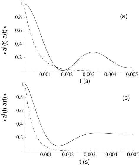
FIG. 1.: A comparison between $\langle a^{{\dagger}}(t)a(t)\rangle$ found using the Born-Markov master equation (dashed line) and the exact solution (solid line). Atom numbers are normalized so that $\langle a^{{\dagger}}(0)a(0)\rangle=1$. Parameters are (a) $\Gamma=1\times 10^{6}\mbox{s}^{-2}$, $\sigma_{k}=10^{6}\mbox{m}^{-1}$ for Gaussian coupling and (b) $|\kappa(k_{0})|^{2}=1.0/\sqrt{2\pi}\mbox{m}\mbox{s}^{-2}$ for broadband coupling. Other parameters are $m=5\times 10^{-26}\mbox{kg}$, $\omega_{0}=2\pi\times 123~{}\mbox{s}^{-1}$.

We have presented results in terms of the Gaussian coupling discussed in Sec. (III). This reflects a possible realistic output coupling method. However from the inequality $t_{s}<t_{D}$ we see that even in the broadband limit, atoms do not couple out of the system in a Born-Markov manner for parameters which correspond to the ones we discuss above. Figure 1b compares the exact and Born-Markov solutions to our model in the broadband limit. In this limit the timescale, $t_{R}$ as defined above tends to zero, thus the first inequality is satisfied. However, the inequality, Eq. (43), fails. This figure demonstrates that even for infinitely broad atom coupling the Born-Markov approximation may fail. The parameters chosen are the same as those for the Gaussian coupling, with a strength of coupling in the exact solutions given by

$$|\kappa(k_{0})|^{2}=\frac{\Gamma}{\sqrt{2\pi}~{}\sigma_{k}}\approx 0.4\mbox{m s}^{-2},$$ (45)

In this case the Born-Markov solution again gives exponential decay. However, the decay constant is now given as the broadband limit of Eq. (25).

Figure 1 demonstrates that for our model of output coupling from an atom laser, results for the number of atoms using the Born-Markov approximations disagree qualitatively with the exact solutions. One of the effects of not being able to ignore the back-action from the reservoir is that for the model we are considering the number of atoms in the cavity does not tend to zero for long times (Figure 1). We discuss reasons for this behaviour in the next section. If effects such as gravity and repulsive interactions are included the cavity number will tend to zero. However, even with these effects included the loss is not exponential and the conclusion that the Born-Markov approximation fails to describe the output coupling remains.

Here, we have demonstrated the failure of the Born-Markov approximation by the use of the particular system variable, $\langle a^{{\dagger}}a\rangle$. However, the problems with using the Born-Markov approximations are not confined to this particular example. For instance, if the output from a BEC is described using a Born-Markov master equation, the resulting long time energy spectrum is Lorentzian. However, if we avoid making the Born-Markov approximations for atoms the exact spectrum may be non-Lorentzian for some values of coupling strength, $\Gamma$, and frequency, $\omega_{0}$ [17].

VI Effect of gravity on the model

In this section we present a quasi-single particle model which allows us to consider the effects of gravity on our output coupling. Such a model cannot be extended to show interesting effects, such as noise suppression due to gain saturation if pumping is added to the model as it does not give information about the general quantum statistics of the output atom field. However, it shows that the inclusion of gravity causes the atom number to asymptote to zero. It does this in a non-exponential way, however, and therefore cannot be modelled by a damping term based on the Born-Markov approximation. Moreover, we demonstrate that the short time behaviour predicted by the models with gravity agree with the exact solutions we have presented earlier which ignore the effects of gravity.

The previous section demonstrated qualitative differences between the exact solution of our model and the solution which uses the Born-Markov approximation. In fact, the exact solution of the model has a stable, nondispersing state which means that not all of the atoms leave the cavity, whereas the approximate solution shows an exponential decay of atoms from the cavity. The presence of the stable state is due to a coherence between the atoms in the cavity and the output modes. The Born-Markov approximation ignores any coherence between the cavity mode and the output modes, and therefore cannot describe any model which produces such features. We now show that such features would be destroyed by gravity.

For coherent dynamics without atom-atom interactions, the multiparticle evolution is identical to the evolution of a single particle [23]. The gravitational term makes it impossible to derive analytical results as in section  II, so we solved the corresponding time-dependent Schrödinger equation numerically. This was done in the position basis rather than the momentum basis for convenience. The Hamiltonian for our system with the inclusion of a gravitational potential is

$$H = H_{s}+H_{r}+H_{sr}+H_{g},$$ (46)

$$H_{s} = \hbar\omega_{0}|\psi_{a}\rangle\langle\psi_{a}|,$$ (47)

$$H_{r} = \frac{\hat{P}^{2}}{2M},$$ (48)

$$H_{sr} = \int~{}dx~{}\left(g^{*}(x)|\psi_{a}\rangle\langle x|~{}+~{}g(x)|x\rangle\langle\psi_{a}|\right),$$ (49)

$$H_{g} = Mg\hat{x}\sin(\theta),$$ (50)

where the coupling function, $g(x)$ is related to $\kappa(k)$ by a Fourier transform,

$$g(x) = \int~{}dk\frac{i\hbar\kappa^{*}(k)~{}e^{ikx}}{\sqrt{2\pi}}.$$ (51)

$\hat{P}$ is the momentum operator. With the term $H_{g}=0$, this model is equivalent to a single particle version of our earlier many particle description, Eq. (2), and produces a time dependance for the probability of finding an atom in the cavity which is identical to $\langle a^{{\dagger}}(t)a(t)\rangle$, found previously. These show a long time steady state in the number of atoms in the cavity which does not tend towards zero. With the inclusion of gravity ($H_{g}\neq 0$), however, the number of atoms decays to zero in a non-exponential manner. This behaviour is shown in Figure 2.

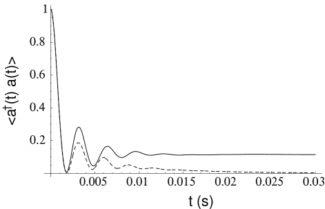
FIG. 2.: The effect of introducing gravity into the model on the number of atoms in the cavity $\langle a^{{\dagger}}(t)a(t)\rangle$. Atom numbers are normalized so that $\langle a^{{\dagger}}(0)a(0)\rangle=1$. The solid line shows the figure with gravity turned off and agrees with the results presented in Fig. 1a. The dashed line includes gravity, $g~{}\mbox{sin}(\theta)$, $g=9.8\mbox{m s}^{-1},\theta=\pi/20$.

In figure 2 we can see collapses and revivals in the number of atoms in the cavity. This is due to the evolving phase relationship between the atoms in the cavity and the atoms which have been coupled into the output field modes. There is no version of the Born-Markov approximation that can describe behaviour such as this, as such an approximation requires that there be no entanglement between the lasing mode and the output modes.

The presence of gravity changes the long time behaviour of our model so that the number of atoms asymptotes to zero, while the short time behaviour remains the same. Other effects may also lead to the long time decay of atom number. Repulsive interactions, for instance, would be expected to destroy the thin stable structure in position space which leads to the long time non-zero population of the cavity mode. The effect of repulsive interactions can be included in this model by including in Eq. (46) a nonlinear Hamiltonian term given by

$$H_{i} = NU_{0}|\psi(x)|^{2}.$$ (52)

Including such interactions into our model produces a Gross-Pitaevskii type equation [21], where $N$ is the number of atoms in the system and $U_{0}$ an interaction strength. We find that introducing such an interaction term does cause the atom number to go below the nonzero steady state predicted in the interaction free model.

VII A non Markovian master equation

In the previous two sections we have shown that the standard master equation does not correctly describe the dynamics of our model for particular parameters. However a master equation, in terms of only the system variables, would be an important tool for describing an atom laser. We now consider whether a non-Markovian master equation can give a correct description of the atom laser. To do this, we continue to make the Born approximation, but do not make a Markov approximation.

The master equation with the Born approximation only is given in Eq. (21). Again, we check the validity of the Born approximation by comparing the results obtained from this Born master equation with the exact solutions. We begin by considering the resulting equation for the expectation value $\langle a^{{\dagger}}\rangle$,

$$\frac{d\langle a^{{\dagger}}(t)\rangle}{dt} = i\omega_{0}\langle a^{{\dagger}}\rangle(t)-\int_{0}^{t}dt^{\prime}\langle a^{{\dagger}}(t^{\prime})\rangle\times$$ (54)

$$\int|\kappa(k)|^{2}e^{i\omega_{k}(t-t^{\prime})}dk,$$

Eq. (54) is the same as that obtained through the full system plus reservoir equations given in Eq. (7). This can be seen by making the transformation $\tau=t-t^{\prime}$ in Eq. (54) to obtain the alternative form, Eq. (7). Despite this success, the density operator equation with the Born approximation, Eq. (21) is not correct. In particular, the Born approximation does not give correct values for higher order expectation values, such as $\langle a^{{\dagger}}a\rangle$.

The equation derived from the non-Markovian master equation, Eq. (21) for the number operator expectation value is

$$\frac{d\langle a^{{\dagger}}(t)a(t)\rangle}{dt} = -\int_{0}^{t}d\tau\langle a^{{\dagger}}a\rangle(t-\tau)\times$$ (56)

$$\int|\kappa(k)|^{2}e^{i(\omega_{0}-\omega_{k})\tau}dk+\mbox{h.c},$$

with solution

$$\langle a^{{\dagger}}(t)a(t)\rangle=\langle a^{{\dagger}}(0)a(0)\rangle\times$$ (58)

$${\cal L}^{-1}\left\{\frac{1}{s+{\cal L}\left\{f^{\prime}(t)\right\}(s)+{\cal L}\left\{f^{\prime}(t)^{*}\right\}(s)}\right\}(t).$$

These do not agree with the corresponding exact equations given in Eq. (9) and Eq. (12), as is shown in Fig. 3.

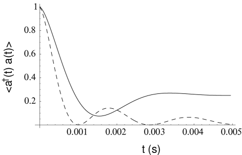
FIG. 3.: A comparison between $\langle a^{{\dagger}}(t)a(t)\rangle$ found using the Born (non-Markovian) master equation (dashed line) and the exact solution (solid line) respectively in the broadband regime. Atom numbers are normalized so that $\langle a^{{\dagger}}(0)a(0)\rangle=1$. Parameters are the same as in Fig. 1b.

This figure compares the exact results for $\langle a^{{\dagger}}(t)a(t)\rangle$ with the solution in the Born approximation only, Eq. (58). The parameter values chosen are the same as those discussed in section V and the comparison is made for broadband coupling. The reason for the failure of the non-Markovian master equation is that where the correct equations lead to the term $\langle a^{{\dagger}}(t)e^{-i\omega_{0}\tau}a(t-\tau)\rangle$, the non-Markovian master equation with the Born approximation leads to $\langle a^{{\dagger}}(t-\tau)a(t-\tau)\rangle$. These two terms are equal if we consider only the free evolution of the system, and ignore the interaction term. That is, to zeroth order in $|\kappa(k)|^{2}$, $\langle a^{{\dagger}}(t-\tau)a(t-\tau)\rangle\approx\langle a^{{\dagger}}(t)a(t-\tau)\rangle(t)e^{-i\omega_{0}t}$. However, there are interaction terms between the system and reservoir. Due to the interaction, terms obtained using the Born approximation are not equal to the exact results. To reproduce equations for the correct system dynamics we cannot ignore the correlations which arise between the system and reservoir.

In optics the Born-Markov approximation is a useful approximation in almost all practical parameter regimes. In fact, in optics the value of $\omega_{0}$ is sufficiently large that, if one assumes a linear dispersion relation the reservoir correlation can be well approximatied by a Dirac delta function. This is not the case for atoms.

The non-Markovian master equation, Eq. (21), gives correct results for single operator expectation values. Nevertheless, the Born approximation neglects higher orders in the interaction term, $|\kappa(k)|^{2}$, thus ignoring reservoir evolution. This leads to incorrect results for higher order expectation values, such as $\langle a^{{\dagger}}(t)a(t)\rangle$.

VIII Conclusion

We have discussed the use of master equations and other density operator equations for atom lasers. We find that the Born-Markov master equation, as is commonly used in optics, is not valid in parameter regimes in which atom lasers may work. The output modes correlation function for photons is well approximated by a delta function in the broadband limit, and for typical optical parameters. In comparison, this function falls off as $1/\sqrt{\tau}$ for atoms because of the atom dispersion relations.

The Born-Markov approximations must be made self consistently. In regimes where the Born-Markov approximations fail, the system can be solved in the Heisenberg picture, treating the output modes fully [16, 17]. For broadband coupling, the parameter regimes in which the Born-Markov approximation is valid is given in Eq. (43). Another possibility for describing such systems involves the use of quantum trajectories. These have been found to be useful for other systems in which no Born-Markov master equation exists[22].

The breakdown of the Born and Markov approximations means that new theoretical methods will be required to understand the atom laser in some regimes. However, it also opens up the possibility of finding new properties of atom lasers significantly different from those found in the optical laser.

REFERENCES

- [1] Email address: Glenn.Moy@anu.edu.au
- [2] M. Holland, K. Burnett, C. Gardiner, J.I. Cirac and P.Zoller, Phys. Rev. A 54, R1757 (1996).
- [3] H.M. Wiseman and M.J.Collett, Physics Lett. A 202,246 (1995).
- [4] H.M. Wiseman, A. Martin, and D.F. Walls, Quantum Semiclass. Opt. 8, 737 (1996).
- [5] A.M. Guzman, M. Moore, and P.Meystre, Phys. Rev. A53, 977 (1996).
- [6] R.J.C. Spreeuw, T. Pfau, U. Janicke and M. Wilkens, Europhysics Letters 32, 469 (1995).
- [7] M. Olshanii, Y. Castin and J. Dalibard, Proc. of the 12th Int. Conference on Laser Spectroscopy, edited by M. Inguscio, M. Allegrini and A. Sasso. (1995).
- [8] G.M. Moy, J.J. Hope, and C.M. Savage, Phys. Rev. A55,3631 (1997).
- [9] H. Wiseman, Phys. Rev. A56,2068 (1997).
- [10] see for example D. Walls, G. Milburn, Quantum Optics (Springer-Verlag, Berlin, 1994).
- [11] M.J. Collett and C.W. Gardiner, Phys. Rev. A30, 1386 (1984).
- [12] M.R. Andrews, C.G. Townsend, H.J. Miesner, D.S. Durfee, D.M.Kurn, and W.Ketterle, Science 275,637 (1997).
- [13] M.O. Mewes, M.R. Andrews, D.M. Kurn, D.S. Durfee, C.G.Townsend, and W.Ketterle, Phys. Rev. A78,582 (1997).
- [14] M.O. Mewes et al., Phys. Rev. Lett.77,416 (1996).
- [15] see for example K. Huang, Statistical Mechanics (John Wiley and Sons, New York, 1987).
- [16] J.J. Hope, Phys. Rev. A55, 2531 (1997).
- [17] G.M. Moy and C.M. Savage, Phys. Rev. A56,1087 (1997).
- [18] H. Carmichael, An open systems approach to quantum optics (Springer-Verlag, Berlin, 1991).
- [19] W. Louisell, Quantum statistical properties of radiation (Wiley Interscience publications, 1990).
- [20] C. Cohen-Tannoudji et al, Atom Photon Interactions (Wiley Interscience publications, 1992).
- [21] E. M. Lifshitz, and L.P. Pitaevskii, Statistical Physics (Pergamon Press, Oxford, 1980), Pt2.
- [22] S. Bay, P. Lambropoulos, and K. Molmer, Phys. Rev. Lett.79, 14 (1997).
- [23] M.A. Kasevich and S.E. Harris, Optics Letters 21, 677 (1996).