Linear quantum trajectories: Applications to continuous projection measurements

Abstract

We present a method for obtaining evolution operators for linear quantum trajectories. We apply this to a number of physical examples of varying mathematical complexity, in which the quantum trajectories describe the continuous projection measurement of physical observables. Using this method we calculate the average conditional uncertainty for the measured observables, being a central quantity of interest in these measurement processes.

I Introduction

Quantum master equations, which govern the evolution of a density matrix representing the state of a physical system, have a wide application in quantum dissipation and continuous measurement theory BHE ; Arg ; WandM . They describe the evolution of a quantum system that is interacting with an environment which, due to the interaction, may absorb energy from the system (dissipation), and will continually provide information about the state of the system (continuous measurement). A classic example of a system interacting with an environment is that of a single mode of an optical cavity which is allowed to leak out of the cavity via an imperfect end-mirror. The photons in the cavity leak out over time, and these may be detected with a photo-detector. The environment consists of the continuum of optical modes outside the cavity, and provides a mechanism for dissipation and continuous measurement. A master equation would describe the evolution of the system averaged over all the possible times at which the photons may be detected leaving the cavity. However, the master equation may be rewritten in an equivalent form as a stochastic equation which describes the evolution of the system for each set of photo-detection times nonLSE . Each possible realisation of the stochastic equation corresponds to a set of detection times, or more generally, to a particular set of measurement results. Each set of results is termed a quantum trajectory Hcarm , and the stochastic equation is said to unravel the master equation. The kind of stochastic process appearing in the equation will depend upon the kind of measurement process. For photo-detection of the output of a cavity mode the stochastic process is a point process Point , while for homodyne detection it is a Wiener process StochMeth . However, the master equation, giving the overall average evolution, does not depend upon the choice of measurement. In other words, there are many different ways to unravel any particular master equation. Here we will be concerned with stochastic equations which contain the Wiener process.

The fact that quantum master equations may be rewritten as Linear Stochastic Equations (LSE’s) for the quantum state vector, referred to alternatively as linear quantum trajectories, has been known in the mathematical physics literature for some time mathLSE , but has only fairly recently seen exposure in the physics literature GandG ; HMWetc ; Strunz , where it has been common to use non-linear stochastic equations solNLSE ; BS . The advantage of writing master equations as LSE’s, rather than the more familiar non-linear version, is that in certain cases it has been found that explicit evolution operators corresponding to these equations may be obtained in a straightforward manner. However, as far as we are aware, the only method that has been used to obtain evolution operators for these equations to date is to choose an initial state which allows the stochastic equation for the state to be written as a stochastic equation for an eigenvalue, or which simplifies the action of the evolution operator GandG ; HMWetc . In this paper we present a more general method for obtaining explicit evolution operators for these equations which makes no reference to the initial state. Naturally the resulting evolution operators contain classical random variables. The complexity of the stochastic equations which govern these classical random variables depends upon the complexity of the commutation relations between the operators appearing in the LSE. If the complexity of the commutation relations is sufficiently high then the stochastic equations governing the classical random variables become too complex to solve analytically. Nevertheless, even if this is the case, the form of the evolution operator provides information regarding the type of states produced by the LSE, and the problem is reduced to integrating the classical stochastic equations numerically. We also note that the solution to an LSE provides additional information to that contained in the solution to the equivalent master equation, because it gives the state of the system for each trajectory. For example, the variance of a system operator may be calculated for each final state (ie. for each trajectory), and this is referred to as the conditional variance as it is conditional upon the results of the measurement. The overall average of these variances may be then be calculated. The solution to the master equation allows us to calculate only the variance which is obtained by first averaging the final states over all trajectories, which is, in general, quite a different quantity.

In the following we use as examples LSE’s corresponding to the continuous measurement of physical observables. A term of the form

$$\dot{\rho}=\cdots-k[O,[O,\rho]]\cdots$$ (1)

in a quantum master equation for the evolution of a density matrix, $\rho$, for a quantum system $S$, describes a continuous projection measurement of an observable $O$ of $S$. The rate at which information is gained regarding the observable is determined by $k$ which is a positive constant. That a continuous measurement of a physical observable can be described in this way has been demonstrated by Barchielli and co-workers Barchielli , and also by Ueda et al. Ueda using a quite different approach. For the theory of continuous measurement the reader is referred to these works and references cm0 ; cm1 ; cm2 ; cm3 . We refer to this measurement process as a continuous projection measurement because in the absence of any system evolution, the sole effect of this term is to reduce the off-diagonal elements of the density matrix to zero in the eigenbasis of that observable. That is, it describes, in the long time limit, a projection onto one of the eigenstates of the observable under observation. If, in addition, the observable commutes with the Hamiltonian describing the free evolution of the system under observation, then the free evolution does not interfere with this process of projection, and the measurement is referred to as a continuous Quantum Non-Demolition (QND) measurement QNDdefn ; WandM .

Before we proceed we note the following points. The LSE which is equivalent to the general master equation Lindblad

$$\dot{\rho}=-\frac{i}{\hbar}[H,\rho]+\sum_{n=1}^{N}(2O_{n}\rho O^{\dagger}_{n}-O^{\dagger}_{n}O_{n}\rho-\rho O^{\dagger}_{n}O_{n}),$$ (2)

where $H$ is Hermitian and the $O_{n}$ are arbitrary operators, is

$$d|\psi\rangle=\left[-\frac{i}{\hbar}Hdt-\sum_{n=1}^{N}(O^{\dagger}_{n}O_{n}dt-\sqrt{2}O_{n}dW_{n}(t))\right]|\psi\rangle,$$ (3)

where the $dW_{n}(t)$ are independent stochastic Wiener increments which obey the Ito calculus relation $dW_{n}(t)^{2}=dt$ StochMeth .

During evolution an initialy pure quantum state remains pure, but changes in a random way determined by the values taken by the Wiener process. The state at time $t$, $|\psi(t)\rangle_{\mbox{\scriptsize w}}$, is not normalised, and the probability measure for the system to have evolved to that particular state at that time is given by GandG

$$\langle\psi(t)|\psi(t)\rangle_{\mbox{\scriptsize w}}\mbox{d}P_{\mbox{\scriptsize w}},$$ (4)

where $\mbox{d}P_{\mbox{\scriptsize w}}$ is the Wiener measure. That is, it is the joint probability measure for all the random variables that appear in the expression for $|\psi(t)\rangle_{\mbox{\scriptsize w}}$. It follows therefore that moments of system operators calculated with the equivalent master equation at time $t$ are given by the expression

$$\langle{\cal O}\rangle=\int\langle\psi(t)|{\cal O}|\psi(t)\rangle_{\mbox{\scriptsize w}}\mbox{d}P_{\mbox{\scriptsize w}}.$$ (5)

where ${\cal O}$ is the system operator in question, and $\mbox{d}P_{\mbox{\scriptsize w}}$ represents integration over all possible values of the random variables. For an in-depth account of LSE’s and their relationship to physical measurements we refer the reader to reference GandG .

II Obtaining Evolution Operators for Linear Quantum Trajectories

II.1 General method

We will explicitly treat here LSE’s which contain only one stochastic increment. However it will be clear that this treatment may be easily extended for multiple stochastic increments. Let us write a general LSE with a single stochastic increment as

$$d|\psi\rangle=(\tilde{A}\;dt+B\;dW(t))|\psi\rangle.$$ (6)

In this equation $\tilde{A}$ and $B$ are arbitrary operators. We will see that the complexity of the evolution operator will depend upon the complexity of the commutation relations between $\tilde{A}$ and $B$.

Let us define the integral of Wiener increments over a time $\Delta t$ as $\Delta W(t)$. The probability density for $\Delta W(t)$ is StochMeth

$$P(\Delta W(t))=\frac{1}{\sqrt{2\pi\Delta t}}e^{-(\Delta W(t))^{2}/(2\Delta t)},$$ (7)

so that $\langle\Delta W(t)\rangle=0$ and $\langle(\Delta W(t))^{2}\rangle=\Delta t$. As a first step in obtaining an evolution operator for the LSE in Eq.(6) we rewrite it in the form

$$|\psi(t+dt)\rangle = e^{(\tilde{A}-(B^{2}/2))dt}e^{BdW(t)}|\psi\rangle$$ (8)

$$= e^{Adt}e^{BdW(t)}|\psi\rangle,$$

were we have defined $A=\tilde{A}-B^{2}/2$. It is easily verified that this is correct to first order by expanding the exponentials to second order and using the Ito calculus relation $dW(t)^{2}=dt$. To first order the state at time $t+\Delta t$ is therefore

$$|\psi(t+\Delta t)\rangle=e^{A\Delta t}e^{B\Delta W(t)}|\psi(t)\rangle,$$ (9)

so that the state at time $t$ may be written

$$|\psi(t)\rangle_{\mbox{\scriptsize w}}=\lim_{\Delta t\rightarrow 0}\prod_{n=1}^{N}(e^{A\Delta t}e^{B\Delta W_{n}})\;|\psi(0)\rangle,$$ (10)

where

$$\Delta W_{n}=\int_{(n-1)\Delta t}^{n\Delta t}\!\!\!\!\!\!\!\!\!\!\!\!dW(t),$$ (11)

and $N\rightarrow\infty$ as $\Delta t\rightarrow 0$ so that $N\Delta t=t$ is always true. To complete the derivation of the evolution operator we must take the limit in Eq.(10). To do this we must combine the arguments of the exponentials which appear in the product, so that we may sum the infinitessimals. We will choose to do this by first repeatedly swapping the order of the exponentials containing the operator $A$ with those containing the operator $B$. The simplest case occurs when $A$ and $B$ commute so that the problem essentially reduces to the single variable case, and we treat this in Sec.II.2. The simplest non-trivial case occurs when the commutator $[A,B]$, while non-zero, commutes with both $A$ and $B$, and we treat this in Sec.II.3. In the final part of this section we examine a more complicated example in which the commutator $[A,B]$ does not commute with either $A$ or $B$.

II.2 A QND measurement of photon number

The mathematically trivial case occurs when $A$ and $B$ commute. A non-trivial physical example to which this corresponds is a QND measurement of the photon number of a single cavity mode. Denoting the annihilation operator describing the mode by $a$, the free cavity field Hamiltonian is given by WandM

$$H=\hbar\omega(a^{\dagger}a+\frac{1}{2}),$$ (12)

in which $\omega$ is the frequency of the cavity mode, and the observable to be measured is $O=a^{\dagger}a$. With this we have

$$A = -i\omega(a^{\dagger}a+\frac{1}{2})-2k(a^{\dagger}a)^{2},$$ (13)

$$B = \sqrt{2k}a^{\dagger}a,$$ (14)

in which $k$ is the measurement constant introduced in Eq.(1). As $A$ and $B$ commute the exponentials in Eq.(10) combine trivially and we obtain

$$|\psi(t)\rangle_{\mbox{\scriptsize w}} = \lim_{\Delta t\rightarrow 0}e^{AN\Delta t}\exp\left[{B\sum_{n}\Delta W_{n}}\right]\;|\psi(0)\rangle$$ (15)

$$= e^{At}e^{BW(t)}\;|\psi(0)\rangle.$$

As the Wiener process, $W(t)$, is a sum of independent Gaussian distributed random variables, $W_{n}$, it is naturally Gaussian distributed, the mean and variance of $W(t)$ being zero and $t$ respectively. In a particular realisation of the stochastic equation Eq.(6), the Wiener process will have a particular value at each time $t$, and as we mentioned above, the set of all these values corresponds to the trajectory that is taken by that particular realisation. The fact that to obtain the state at time $t$ we require only the value of the Wiener process at that time means that we do not require all the trajectory information, but just a single variable associated with that trajectory. For more complicated cases, in which the operators do not commute, we will find that other variables associated with the trajectory appear in the evolution operator.

As the situation we consider here is a QND measurement, the phase uncertainty introduced by the measurement of photon number does not feed back to affect the measurement, so that the result is simply to decrease continuously the uncertainty in photon number, and the state of the system as $t$ tends to infinity tends to a number state. If we denote the evolution operator derived in Eq.(15) by $V(t)$, and start the system in an arbitrary mixed state $\rho(0)$, then at time $t$ the normalised state of the system may be written

$$\rho(t)=\frac{V(t)\rho(0)V^{\dagger}(t)}{\mbox{Tr}\left\{V(t)\rho(0)V^{\dagger}(t)\right\}}.$$ (16)

As $V(t)$ is diagonal in the photon number basis, we only require the diagonal elements of the initial density matrix to calculate moments of the photon number operator. Denoting the diagonal elements of the initial density matrix by $\rho_{n}$, and the diagonal elements of $V(t)V^{\dagger}(t)$ by $V_{n}$, the variance of the photon number, for a given trajectory, is given by

$$\sigma_{\scriptsize n}^{2}(t)_{\mbox{\scriptsize w}}=\frac{\sum_{n}n^{2}\rho_{n}V_{n}}{\sum_{n}\rho_{n}V_{n}}-\frac{\left(\sum_{n}n\rho_{n}V_{n}\right)^{2}}{\left(\sum_{n}\rho_{n}V_{n}\right)^{2}}.$$ (17)

The uncertainty in our knowledge of the number of photons is the square root of this variance. Averaging this uncertainty over all trajectories therefore tells us, on average, how accurately we will have determined the number of photons at a later time. To calculate the value of the uncertainty for each trajectory, averaged over all trajectories we must multiply $\sigma_{\scriptsize n}(t)_{\mbox{\scriptsize w}}$ by the probability for each final state and average over all the final states. The probability measure for the final states, $\rho(t)$, is given by the Wiener measure multiplied by the norm of the final state, $\mbox{Tr}\left\{V(t)\rho(0)V^{\dagger}(t)\right\}$. This probability measure is not in general Gaussian in $W(t)$, but a weighted sum of Gaussians, one for each $n$. Performing the multiplication, we obtain the average conditional uncertainty in photon number as

$$\langle\sigma_{\scriptsize n}(t)_{\mbox{\scriptsize w}}\rangle=\int\sqrt{\sum_{nm}n(m-n)\rho_{n}\rho_{m}V_{n}V_{m}}\;\mbox{d}P_{\mbox{\scriptsize w}},$$ (18)

in which

$$V_{n} = e^{-4ktn^{2}+2\sqrt{2k}nW},$$ (19)

$$\mbox{d}P_{\mbox{\scriptsize w}} = \frac{1}{\sqrt{2\pi t}}e^{-W^{2}/(2t)}\mbox{d}W.$$ (20)

We note that $\langle\sigma_{\scriptsize n}(t)_{\mbox{\scriptsize w}}\rangle$ may be written as a function of $\tau=kt$, being the time scaled by the measurement constant. Hence, as we expect, increasing the measurement time has the same effect on $\langle\sigma_{\scriptsize n}(t)_{\mbox{\scriptsize w}}\rangle$ as increasing the measurement constant. We evaluate $\langle\sigma_{\scriptsize n}(\tau)_{\mbox{\scriptsize w}}\rangle$ numerically for an initial thermal state, and an initial coherent state, and display the results in figure 1. We have chosen the initial states so that they have the same uncertainty in photon number, with the result that the mean number of photons in each of the two states is quite different. The results show the decrease in uncertainty with time, which is seen to be only weakly dependent upon the initial state.

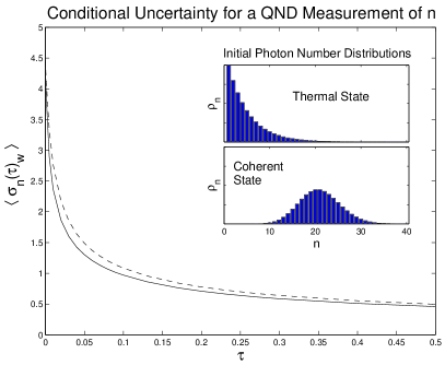
Figure 1: The conditional uncertainty in photon number averaged over all trajectories, $\langle\sigma_{n}(t)_{\mbox{\scriptsize w}}\rangle$, is plotted here against the dimensionless scaled time, $\tau=kt$. The dotted line corresponds to an initial coherent state, and the solid line to an initial thermal state. Both initial states were chosen to have $\sigma_{n}^{2}=20$, giving the thermal state a mean photon number of $\langle n\rangle=4$, and the coherent state a mean photon number of $\langle n\rangle=20$. The photon number distributions for the two initial states are displayed in the inset.

II.3 A measurement of momentum in a linear potential

The simplest mathematically non-trivial case occurs when the commutator between $A$ and $B$, while non-zero, is such that it commutes with both $A$ and $B$. A physical situation to which this corresponds is a continuous measurement of the momentum of a particle in a linear potential. If we denote the position and momentum operators for the particle as $Q$ and $P$ respectively, then the Hamiltonian is given by

$$H=\frac{1}{2m}P^{2}-FQ,$$ (21)

in which $m$ is the mass of the particle and $F$ is the force on the particle from the linear potential. In this case we have

$$A = (\frac{-i}{2\hbar m}-2k)P^{2}+\frac{iF}{\hbar}Q,$$ (22)

$$B = \sqrt{2k}P,$$ (23)

in which $k$ is again the measurement constant.

Returning to Eq.(10) we see that to obtain a solution we must pass all the exponentials containing the operator $B$ to the right through the exponentials containing the operator $A$. In order to perform this operation we need a relation of the form

$$e^{B}e^{A}=e^{A}e^{C}.$$ (24)

For the present case the required relation is simply given by the Baker-Campbell-Hausdorff formula BCH ; BHE

$$e^{B}e^{A}=e^{A}e^{B}e^{-[A,B]}.$$ (25)

Using this relation to propagate successively all of the exponentials containing $B$ to the right in the product in Eq.(10) we obtain

$$\prod_{n=1}^{N}(e^{A\Delta t}e^{B\Delta W_{n}})=\exp\left[{AN\Delta t}\right]\exp\left[{B\sum_{n=1}^{N}\Delta W_{n}}\right]$$

$$\times\exp\left[{-[A,B]\Delta t\sum_{n=1}^{N}(n-1)\Delta W_{n}}\right].$$ (26)

All that remains is to calculate the joint probability density for the random variables. The first is the Wiener process, and the second is

$$Y(t) = \lim_{\Delta t\rightarrow 0}\Delta t\sum_{n=1}^{N}(n-1)\Delta W_{n}=\int_{0}^{t}t^{\prime}dW(t^{\prime}).$$ (27)

Clearly these are both Gaussian distributed with zero mean and all that we require is to calculate the covariances $\langle Y(t)^{2}\rangle$ and $\langle W(t)Y(t)\rangle$ to determine completely the joint density at time $t$. Using $\langle\Delta W_{n}\Delta W_{n}\rangle=\delta_{nm}\Delta t$ these quantities are easily obtained:

$$\langle Y(t)^{2}\rangle = \lim_{\Delta t\rightarrow 0}\Delta t\sum_{n=1}^{N}((n-1)\Delta t)^{2}\Delta t$$ (28)

$$= \int_{0}^{t}t^{\prime 2}\;dt^{\prime}=t^{3}/3,$$

$$\langle W(t)Y(t)\rangle = \lim_{\Delta t\rightarrow 0}\sum_{n=1}^{N}((n-1)\Delta t)\Delta t$$ (29)

$$= \int_{0}^{t}t^{\prime}\;dt^{\prime}=t^{2}/2.$$

The state at time $t$, under the evolution described by the stochastic equation, is therefore

$$|\psi(t)\rangle_{\mbox{\scriptsize w}}=e^{At}e^{BW(t)}e^{-[A,B]Y(t)}|\psi(0)\rangle,$$ (30)

where the joint probability density for $W$ and $Y$ at time $t$ is given by

$$P_{\mbox{\scriptsize w}}(W,Y)=\left(\frac{\sqrt{12}}{2\pi t^{2}}\right)\exp\left[-\frac{2}{t}W^{2}-\frac{6}{t^{3}}Y^{2}+\frac{6}{t^{2}}WY\right].$$

Note that to obtain the probability density for the final state, this must be multiplied by the norm of the state at time $t$.

Returning to the specific case of a particle in a linear potential, we may now obtain results for various quantities of interest. Writing the evolution operator in terms of the momentum and position operators we have

$$|\psi(t)\rangle_{\mbox{\scriptsize w}} = \exp\left[{((\frac{-i}{2\hbar m}-2k)P^{2}+\frac{iF}{\hbar}Q)t}\right]$$ (31)

$$\times \exp\left[\sqrt{2k}(PW(t)+FY(t))\right]|\psi(0)\rangle.$$

Using the Zassenhaus formula Witschel to disentangle the argument of the first exponential we may rewrite this in the more convenient form

$$|\psi(t)\rangle_{\mbox{\scriptsize w}} = \exp\left[{\frac{iF}{\hbar}Qt}\right]\exp\left[{\eta(-P^{2}t-PFt^{2}-F^{2}t^{3}/3)}\right]$$ (32)

$$\times \exp\left[{\sqrt{2k}(PW(t)+FY(t))}\right]|\psi(0)\rangle,$$

in which $\eta=(\frac{i}{2\hbar m}+2k)$. For those not familiar with the Zassenhaus formula, it is complementary to the BCH formula. While the BCH formula shows how to write an exponential of the sum of two operators as a product of exponentials of the operators and their commutator (or in more complicated cases repeated commutators of the two operators), the Zassenhaus formula shows how to write the product of exponentials of two operators as the exponential of the sum of the operators and repeated commutators.

Let us first take an arbitrary initial state, writing it in the momentum eigenbasis so that we have

$$|\psi(0)\rangle=\int_{-\infty}^{\infty}\!\!\!\!\!\Psi(p)|p\rangle\;\mbox{d}p\;\;,\;\;\;\int_{-\infty}^{\infty}\!\!\!\!\!|\Psi(p)|^{2}\;\mbox{d}p=1.$$ (33)

Using Eqs.(32) and (33) in Eq.(5) to calculate the moments of $p$ given by first averaging over all trajectories (that is, the moments which would be given by the equivalent master equation) we readily obtain

$$\langle p(t)^{n}\rangle=\langle(p(0)+Ft)^{n}\rangle.$$ (34)

In particular, for any initial state, $|\psi(0)\rangle$, the average value of the momentum at time $t$, $\langle p(t)\rangle$, is simply shifted from the initial value by the impulse $Ft$. The variance of the momentum at time $t$, $\sigma_{p}^{2}(t)=\langle p(t)^{2}\rangle-\langle p(t)\rangle^{2}$, remains equal to its original value. That is, the uncertainty introduced into the position of the particle by the momentum measurement does not feed back into the momentum, even though the momentum does not commute with the Hamiltonian. This is because while the momentum determines the position at a later time, the converse is not true. These results for the moments are easily checked using the equivalent master equation.

Now let us consider the conditional variance of the momentum at time $t$ averaged over all trajectories. In the previous section we calculated the conditional uncertainty, being the square root of the variance, and averaged this over all trajectories. Here however, we will find that the conditional variance is independent of the trajectory taken, and depends only on the measurement time. This will also be true of the example which we will treat in the next section. In this case clearly it does not matter if we first average the conditional variance over the trajectories, and then take the square root, or if instead we average the conditional uncertainty, because the averaging procedure is redundant. However, in general the two procedures are not equivalent. We will denote the conditional variance by $\langle\sigma_{p}^{2}(t)_{\mbox{\scriptsize w}}\rangle$. As the uncertainty in position does not feed back into the momentum, we expect that this variance should steadily decrease to zero. This is because during a trajectory our knowledge of the momentum steadily increases so that the distribution over momentum becomes increasingly narrow. To perform this calculation we take the initial state to be the minimum uncertainty wave-packet given by the ground state of a harmonic oscillator of frequency $\omega$. The average values of the position and momentum of the particle are both zero in this state and the respective variances are

$$\langle Q^{2}\rangle = \frac{\hbar}{2m\omega}\equiv\sigma_{Q}^{2}(0)\;\;,\;\;\;\langle P^{2}\rangle=\frac{m\hbar\omega}{2}\equiv\sigma_{p}^{2}(0),$$

and in momentum space the state may be written

$$|\psi(0)\rangle=\left(\frac{1}{\pi m\hbar\omega}\right)^{\frac{1}{4}}\int_{-\infty}^{\infty}\!\!\!\!\!e^{-P^{2}/(2m\hbar\omega)}|p\rangle\;\mbox{d}p.$$ (35)

The moments of momentum for each trajectory are given by

$$\langle p^{n}\rangle_{\mbox{\scriptsize w}}=\frac{\langle\psi(t)|p^{n}|\psi(t)\rangle_{\mbox{\scriptsize w}}}{\langle\psi(t)|\psi(t)\rangle_{\mbox{\scriptsize w}}},$$ (36)

and we calculate the first and second to give $\sigma_{p}^{2}(t)_{\mbox{\scriptsize w}}=\langle p(t)^{2}\rangle_{\mbox{\scriptsize w}}-\langle p(t)\rangle^{2}_{\mbox{\scriptsize w}}$. We obtain

$$\langle\sigma_{p}^{2}(t)_{\mbox{\scriptsize w}}\rangle=\frac{\sigma_{p}^{2}(0)}{1+8k\sigma_{p}^{2}(0)t}.$$ (37)

This is independent of $W$ and $Y$ and hence independent of the trajectory. It is therefore unnecessary to average over the final states. Indeed $\langle\sigma_{p}^{2}(t)_{\mbox{\scriptsize w}}\rangle$ decreases steadily from the initial value to zero as $t\rightarrow\infty$ as we expect from the discussion above. This means that while the average value of momentum is determined by the measurement results, the error in our estimate of the momentum at time $t$ is not.

II.4 A quadrature measurement with a general quadratic Hamiltonian

We now consider an LSE in which the commutator $[A,B]$ does not commute with either $A$ or $B$. As in the previous example, let $P$ and $Q$ be, respectively, the canonical momentum and position operators for a single particle so that they obey the canonical commutation relation $[Q,P]=i\hbar$. With this definition we will take $A$ and $B$ to have the following forms:

$$A = \alpha P^{2}+\gamma Q^{2}+\xi QP+\eta P+\zeta Q,$$ (38)

$$B = kQ+\kappa P,$$ (39)

where $\alpha,\gamma,\eta,\zeta,k$ and $\kappa$ are complex numbers. This example applies to an optical mode of the electromagnetic field, including classical driving and/or classically driven subharmonic generation subharm and for which an arbitrary quadrature is continuously measured. It also applies to the situation of a single particle, which may feel a linear and/or harmonic potential, and which is subjected to continuous observation of an arbitrary linear combination of its position atfm and momentum.

To obtain an evolution operator for the LSE with this choice of the operators $A$ and $B$, we require, as before, a relation of the form given by Eq.(24). To derive this relation we proceed in the following manner.

First we may use the Baker-Campbell-Hausdorff expansion BHE , or alternatively solve the equations of motion given by $dB/d\epsilon=[A,B]$, to obtain an expression for $e^{\epsilon A}Be^{-\epsilon A}$. The result is

$$e^{-\epsilon A}\varepsilon Be^{\epsilon A}=\varepsilon f_{1}(\epsilon)Q+\varepsilon f_{2}(\epsilon)P+\varepsilon f_{3}(\epsilon),$$ (40)

in which

$$f_{1}(\epsilon) = \frac{1}{\lambda}(-2\kappa\gamma+k\xi)S+kC,$$ (41)

$$f_{2}(\epsilon) = \frac{1}{\lambda}(2k\alpha-\kappa\xi)S+\kappa C,$$ (42)

$$f_{3}(\epsilon) = \frac{1}{\lambda^{2}}(k\eta\xi+2k\alpha\zeta-\kappa\zeta\xi-2\kappa\gamma\eta)[C-1]$$ (43)

$$+\frac{1}{\lambda}(k\eta+\kappa\zeta)S.$$

In these expressions $C=\cosh(i\hbar\lambda\epsilon)$, $S=\sinh(i\hbar\lambda\epsilon)$ and $\lambda=\sqrt{\xi^{2}-4\alpha\gamma}$. Using the relation

$$e^{-\epsilon A}f(\varepsilon B)e^{\epsilon A}=f(e^{-\epsilon A}\varepsilon Be^{\epsilon A}),$$ (44)

we obtain from Eq.(40)

$$e^{-\epsilon A}e^{\varepsilon B}e^{\epsilon A}=e^{\varepsilon f_{1}(\epsilon)Q+\varepsilon f_{2}(\epsilon)P}e^{\varepsilon f_{3}(\epsilon)}.$$ (45)

Multiplying both sides of this equation on the left by $e^{\epsilon A}$ we obtain a relation of the form $e^{\varepsilon B}e^{\epsilon A}=e^{\epsilon A}e^{\varepsilon D(\epsilon)}$, as we require.

We see from the above procedure that the relation in Eq.(24) may be obtained so long as a closed form can be found for the solution to the operator differential equation $dB/d\epsilon=[A,B]$. Clearly this is straightforward if this equation is linear in $B$, which is true in the example we have treated here, and is sometimes possible in cases in which the equations are non-linear.

In addition, for this example we also require the BCH relation in the form

$$e^{A}e^{B}=e^{A+B+\frac{1}{2}[A,B]}.$$ (46)

This is so that we can sum up in one exponential the operators that result from swapping $e^{\Delta W_{n}B}$ and $e^{n\Delta tA}$.

Using the expressions derived above, with the replacements $\epsilon=n\Delta t$ and $\varepsilon=\Delta W_{n}$, for each $n$ from 1 to $N$, by repeatedly swapping the exponentials containing $B$ with those containing $A$ as in the previous example, we obtain

$$\lim_{\Delta t\rightarrow 0}\prod_{n=1}^{N}(e^{A\Delta t}e^{B\Delta W_{n}}) = e^{At}e^{X_{1}(t)Q+X_{2}(t)P}$$ (47)

$$\times e^{X_{3}(t)}e^{i\hbar Z(t)},$$

in which the classical stochastic variables $X_{i}$ and $Z$, are given by

$$X_{i}(t) = \int_{0}^{t}\!\!\!f_{i}(t^{\prime})dW(t^{\prime}),$$ (48)

$$Z(t) = \int_{0}^{t}\!\!\!f_{1}(t^{\prime})X_{2}(t^{\prime})dW(t^{\prime})-\int_{0}^{t}\!\!\!f_{2}(t^{\prime})X_{1}(t^{\prime})dW(t^{\prime}),$$

where the expressions for the $f_{i}$ are given above, and the integrals are Ito integrals. The $X_{i}$ are Gaussian distributed with zero mean, and their covariances are easily calculated as in the previous example:

$$\langle X_{i}(t)X_{j}(t)\rangle=\!\!\int_{0}^{t}\!\!\!\!f_{i}(t^{\prime})f_{j}(t^{\prime})\;dt^{\prime}.$$ (49)

In addition, the two-time correlation functions for these variables are also easily obtained analytically. In particular we have

$$\langle X_{i}(t)X_{j}(\tau)\rangle=\!\!\int_{0}^{\mbox{min}(t,\tau)}\!\!\!\!f_{i}(t^{\prime})f_{j}(t^{\prime})\;dt^{\prime}.$$ (50)

However, $Z(t)$ is not Gaussian distributed. We are not aware of an analytic expression for this variable, so that its probability density may have to be obtained numerically. We note in passing, however, that in some cases double stochastic integrals of this kind may be written explicitly in terms of products of Gaussian variables StochMeth . We note also that $Z$ determines only the normalisation of the final state, and not the state itself. The normalised state at time $t$ is therefore independent of $Z$, and we examine the consequences of this in appendix A.

We may now write the state at time $t$ as

$$|\psi(t)\rangle_{\mbox{\scriptsize w}}=e^{At}e^{X_{1}(t)Q+X_{2}(t)P}e^{X_{3}(t)+i\hbar Z(t)}|\psi(0)\rangle.$$ (51)

Hence even though values for averages over all trajectories may in general have to be calculated numerically, the evolution operator provides us with information regarding the type of states that will occur at time $t$. In particular, if the initial state is Gaussian in position (and therefore also Gaussian in momentum), then as each of the exponential operators in the above equation transform Gaussian states to Gaussian states, we see that the state of the system remains Gaussian at all times. The mean of the Gaussian in both position and momentum change with time in a random way determined by the values of the stochastic variables.

We will shortly consider a particular example: that of a harmonic oscillator undergoing a continuous observation of position, and use this evolution operator to calculate the conditional variance for the position at time $t$. We will take the initial state to be a coherent state, which is a Gaussian wave packet. This conditional variance does not depend upon the trajectory, but simply upon the initial state and the measurement time, as indeed we found to be the case for the momentum measurement in section II.3.

Let us first show that for an initial coherent state the conditional variance of any linear combination of position and momentum is independent of the trajectory for all of the cases covered by the evolution operator in Eq.(51). To do this we must calculate the effect of this evolution operator on a coherent state. Clearly the effect of the right-most exponential operator is at most to change the normalisation, which effects neither the average values of position and momentum, nor the respective variances. The effect of the next exponential, being linear in $P$ and $Q$, is calculated in appendix B. We find that it changes the mean values of the position and momentum, and alters the normalisation, but the state remains coherent in that the position variance (and hence the momentum variance) is unchanged. Finally, the effect of the exponential quadratic in $P$ and $Q$ is calculated in appendix B. We find that this operator modifies the position variance. However, as the operator does not contain any stochastic variables, and as the manner in which it changes the position variance is independent of the mean position and momentum, we obtain the result that the effect on the position variance, and hence the variance of any linear combination of position and momentum, is trajectory independent.

Let us now consider a harmonic oscillator in which the position is continuously observed. This situation has been analysed by Belavkin and Staszewski using the equivalent non-linear equations BS . The operators $A$ and $B$ in this case are given by

$$A = \left(\frac{-i}{2\hbar m}\right)P^{2}+\left(\frac{-im\omega^{2}}{2\hbar}-2k\right)Q^{2},$$ (52)

$$B = \sqrt{2k}Q,$$ (53)

in which $m$ is the mass of the particle, $\omega$ is the frequency of the harmonic oscillation, and $k$ is the measurement constant for the continuous observation of position. Taking the initial state to be coherent, and denoting it $|\alpha\rangle$, the initial position wave-function is given by

$$\langle x|\alpha\rangle=\left(\frac{2s^{2}}{\pi}\right)^{1/4}e^{-s^{2}x^{2}+2sx\alpha-\frac{1}{2}(|\alpha|^{2}+\alpha^{2})},$$ (54)

where $s^{2}=m\omega/(2\hbar)$. Using the results in appendix B, we find that the coefficient of $x^{2}$ at a later time $t$ is given by

$$s^{\prime 2}=s^{2}\left[\frac{1-2l}{3-2l}\right]\left[1+2\frac{1-2l}{1+2l}\right]$$ (55)

where

$$l=\frac{-1/2}{rz\coth(z\omega t)+(1+ir)},$$ (56)

and we have defined the parameters

$$z=\sqrt{\frac{2i}{r}-1}\;\;,\;\;\;r=\frac{m\omega^{2}}{2\hbar k}.$$ (57)

After some algebra this may be written as

$$s^{\prime 2}=s^{2}iz\frac{iz\tanh(z\omega t)-1}{\tanh(z\omega t)-iz},$$ (58)

in agreement with that derived by Belavkin and Staszewski. The conditional variance for $x$ at time $t$ is given by

$$\sigma_{x}^{2}(t)_{\mbox{\scriptsize w}}=\frac{1}{4\mbox{\small Re}[s^{\prime 2}]}.$$ (59)

As $t$ tends to infinity, Eq.(58) gives a steady state value for the conditional variance, which is

$$\sigma_{x}^{2}=\frac{1}{4\mbox{\small Im}[z]}=\left(\sqrt{2}s^{2}\sqrt{\sqrt{4/r^{2}+1}+1}\right)^{-1}.$$ (60)

The parameter $r$ is a dimensionless quantity which gives essentially the ratio between the frequency of the harmonic oscillator, and the rate of the position measurement. We may view the dynamics of the position variance as being the result of two competing effects. One is the action of the measurement which is continuously narrowing the distribution in position, and consequently widening the distribution in momentum. The other is the action of the harmonic motion, which rotates the state in phase space, so converting the widened momentum distribution into position. Depending on the relative strengths of these two processes, determined by the dimensionless constant $r$, a steady state is reached in which they balance. If the rate of the measurement is very fast compared to the frequency of the oscillation (corresponding to $r\ll 1$), then the localisation in position is much greater than it would be for an unmonitored oscillator, and in that case we succeed effectively in tracking the position of the particle. However, if the frequency of oscillation is much greater than the rate of localisation do to the measurement, then the steady state position variance remains essentially that of the unmonitored oscillator.

III Conclusion

We have presented a method for obtaining evolution operators for various classes of stochastic equations describing linear quantum trajectories, and applied this to a number of physical examples pertaining to physical systems subjected to the continuous projection measurement of an observable. We have shown how the complexity of the stochastic equations governing the random variables which appear in the evolution operator depends upon the commutation relations between the operators appearing in the LSE. For the case in which both these operators commute with their commutator, probability densities for the random variables may be obtained analytically. We have also shown that in cases in which the commutation relations are more complex it is sometimes still possible to obtain an explicit evolution operator. This is possible even in cases in which the classical stochastic integrals, or equivalently the stochastic equations, governing the random variables which appear in this operator are too complex to solve analytically.

Appendix A Eliminating variables which affect only the final normalisation

We found in section II.4 that not all the random variables which appear in the evolution operator are Gaussian distributed. This result is surprising because it has been shown previously, using the non-linear equations, that for an initial Gaussian state, the probability density for the conditional mean position and momentum, and therefore for the final state, are Gaussian distributed for this case solNLSE . These two results may be reconciled due to the fact that the non-Gaussian variable in the evolution operator given in Eq.(51) affects purely the normalisation of the final state, rather than the state itself.

Let us assume that we have an initial state $|\psi\rangle$, and an evolution operator which is a function of the random variables $X$ and $Z$ (which may in general be vector valued). We let the random variable $Z$ determine only the normalisation of the final state, so that the evolution operator may be written

$$V(X,Z,t)={\cal O}(X,t)f(Z,t),$$ (61)

where ${\cal O}$ is an operator valued function, and $f$ is simply a complex valued function. The unnormalised state at time $t$ is then given by

$$|\psi(t)\rangle_{\mbox{\scriptsize w}}={\cal O}(X,t)f(Z,t)|\psi\rangle.$$ (62)

Clearly once we have normalised that state at time $t$, it is no-longer dependent upon $Z$. In particular the normalised state is given by

$$|\tilde{\psi}(t)\rangle_{\mbox{\scriptsize w}}=\frac{{\cal O}(X,t)|\psi\rangle_{\mbox{\scriptsize w}}}{\sqrt{\langle\psi|{\cal O}^{\dagger}(X,t){\cal O}(X,t)|\psi\rangle_{\mbox{\scriptsize w}}}}.$$ (63)

The probability density for the final state is

$$P(X,Z,t)=\langle\psi(t)|\psi(t)\rangle_{\mbox{\scriptsize w}}P_{\mbox{\scriptsize w}}(X,Z,t),$$ (64)

in which $P_{\mbox{\scriptsize w}}(X,Z,t)$ is the probability density given by the Wiener measure for the variables $X$ and $Z$. However, seeing as the normalised state depends only upon $X$, we require for all calculations only the marginal probability density for $X$. Denoting this marginal density also by $P$, we have

$$P(X,t)=\int P(X,Z,t)\;\mbox{d}Z.$$ (65)

In certain cases the probability measure for the normalised state may therefore be Gaussian, even though the measure for the unnormalised state is not. However, as $P(X,Z,t)$ contains a factor of the norm of $|\psi(t)\rangle_{\mbox{\scriptsize w}}$, the probability measure for the output process will, in general, only be Gaussian if the norm is Gaussian in $X$. Clearly the norm is Gaussian in $X$ for initial Gaussian states in the case we investigate in section II.4.

Appendix B The effect on a coherent state of exponentials linear and quadratic in P and Q

We first calculate the effect of an operator of the form

$$e^{\nu P+\mu Q}$$ (66)

on a coherent state $|\alpha\rangle$. The coherent state is defined as the eigenstate of the annihilation operator $a$, such that

$$a|\alpha\rangle=\alpha|\alpha\rangle,$$ (67)

and

$$a=\sqrt{\frac{m\omega}{2\hbar}}\;x+i\sqrt{\frac{1}{2\hbar m\omega}}\;p.$$ (68)

Here $m$ and $\omega$ are the mass and frequency of a harmonic oscillator which serves for the purposes of defining the coherent state. In particular we are interested in the position wave-function of the result. We therefore wish to calculate

$$\langle x|\psi\rangle=\langle x|e^{\nu P+\mu Q}|\alpha\rangle,$$ (69)

where $|x\rangle$ is an eigenstate of the position operator $Q$ such that

$$Q|x\rangle=x|x\rangle.$$ (70)

Note that in general $|\psi\rangle$ will not be normalised. To perform this calculation we will need the BCH formula given in Eq.(46), and the position wavefunction for a coherent state,

$$\langle x|\alpha\rangle = \left(\frac{2s^{2}}{\pi}\right)^{1/4}e^{-s^{2}x^{2}+2sx\alpha-\frac{1}{2}(|\alpha|^{2}+\alpha^{2})}$$ (71)

$$= \left(\frac{2s^{2}}{\pi}\right)^{1/4}e^{-s^{2}x^{2}+2sx\alpha-\alpha_{r}^{2}-i\alpha_{r}\alpha_{i}}$$

where

$$s = \sqrt{\frac{m\omega}{2\hbar}}$$ (72)

$$\alpha = \alpha_{r}+i\alpha_{i}.$$ (73)

Note that this expression contains the phase factor $-i\alpha_{r}\alpha_{i}$. This is left out in many texts, but is essential for consistency with the completeness relations for the position states. We also require the inner product of two coherent states,

$$\langle\alpha|\beta\rangle=e^{-\frac{1}{2}(|\alpha|^{2}+|\beta|^{2})+\alpha^{*}\beta},$$ (74)

and the well known integral formula

$$\int e^{-\alpha x^{2}-\beta x}\;\mbox{d}x=\sqrt{\frac{\pi}{\alpha}}e^{\beta^{2}/(4\alpha)}\;\;,\;\;\mbox{Re}[\alpha]>0.$$ (75)

We proceed first by rewriting the exponential in terms of annihilation and creation operators, so that we have

$$e^{\nu P+\mu Q}=e^{\theta a+\phi a^{\dagger}}=e^{\phi a^{\dagger}}e^{\theta a}e^{\theta\phi/2}$$ (76)

in which

$$\theta=\left(\nu\sqrt{\frac{\hbar}{2m\omega}}-i\mu\sqrt{\frac{m\hbar\omega}{2}}\right)=\phi^{*}.$$ (77)

We may now use the completeness relation for the coherent states to obtain

$$\langle x|\psi\rangle = \langle x|e^{\phi a^{\dagger}}e^{\theta a}|\alpha\rangle e^{\theta\phi/2}$$ (78)

$$= \frac{1}{\pi}\int\!\!\!\!\int\langle x|\beta\rangle\langle\beta|e^{\phi a^{\dagger}}e^{\theta a}|\alpha\rangle e^{\theta\phi/2}\;\mbox{d}^{2}\beta$$

$$= \frac{1}{\pi}\int\!\!\!\!\int\langle x|\beta\rangle\langle\beta|\alpha\rangle\;e^{\theta\alpha+\phi\beta^{*}+\theta\phi/2}\;\mbox{d}^{2}\beta$$

$$= \langle x|\alpha+\phi\rangle e^{\frac{1}{2}|\phi|^{2}+\mbox{\scriptsize Re}[\alpha\phi^{*}]+\theta\alpha+\theta\phi/2}.$$

We see that the state remains coherent, although it is no longer normalised, and is shifted in phase space by $\phi$.

We now wish to calculate the effect of an operator of the form

$$e^{\eta P^{2}+\zeta Q^{2}+\xi QP}$$ (79)

on a coherent state. This time we require to calculate

$$\langle x|\psi\rangle=\langle x|e^{\eta P^{2}+\zeta Q^{2}+\xi QP}|\alpha\rangle.$$ (80)

For this calculation we will need the disentangling theorem for the exponential of a general quadratic form of the annihilation and creation operators, which is given by mjcollett

$$e^{ua^{2}+va^{\dagger 2}+wa^{\dagger}a}=e^{(\chi-w)/2}e^{la^{\dagger 2}}e^{\chi a^{\dagger}a}e^{ma^{2}},$$ (81)

in which

$$l = \frac{v}{f\coth(f)-w}$$ (82)

$$\chi = \ln\left(\frac{f}{f\cosh(f)-w\sinh(f)}\right)$$ (83)

$$m = \frac{u}{f\coth(f)-w}$$ (84)

$$f = \sqrt{w^{2}-4uv}.$$ (85)

First of all rewriting the exponential containing $P$ and $Q$ as an exponential in the annihilation and creation operators, we have

$$\langle x|e^{\eta P^{2}+\zeta Q^{2}+\xi QP}|\alpha\rangle=\langle x|e^{ua^{2}+va^{\dagger 2}+wa^{\dagger}a+u}|\alpha\rangle$$ (86)

in which

$$u = v^{*}=\left(\frac{\zeta\hbar}{2m\omega}-\frac{\eta m\hbar\omega}{2}-i\frac{\xi\hbar}{2}\right)$$ (87)

$$w = \left(\frac{\zeta\hbar}{m\omega}+\eta m\hbar\omega\right).$$ (88)

We now proceed by using the disentangling theorem, and employing the completeness relation for the coherent states.

$$\langle x|\psi\rangle = \langle x|e^{(w+\chi)/2}e^{la^{\dagger 2}}e^{\chi a^{\dagger}a}e^{ma^{2}}|\alpha\rangle$$ (89)

$$= \frac{1}{\pi}\int\!\!\!\!\int\langle x|\beta\rangle\langle\beta|e^{(w+\chi)/2}e^{la^{\dagger 2}}e^{\chi a^{\dagger}a}e^{ma^{2}}|\alpha\rangle\;\mbox{d}^{2}\beta$$

$$= \frac{1}{\pi}\int\!\!\!\!\int\langle x|\beta\rangle\langle\beta|\alpha e^{\chi}\rangle\;e^{l\beta^{*2}}\;\mbox{d}^{2}\beta$$

$$\;\;\times\;e^{\frac{1}{2}|\alpha|^{2}(|e^{2\chi}|-1)+m\alpha^{2}}e^{(\chi-w)/2}.$$

Performing the integral over the real and imaginary parts of $\alpha$, we obtain

$$\langle x|\psi\rangle = \frac{1}{\sqrt{1+2l}}\left(\frac{2s^{2}}{\pi}\right)^{\frac{1}{4}}\!\!\!e^{-\frac{1}{2}|\alpha|^{2}-m\alpha^{2}}e^{(\chi-w)/2}$$ (90)

$$\times\exp\left\{-s^{2}x^{2}\left[\frac{1-2l}{3-2l}\right]\left[1+2\frac{1-2l}{1+2l}\right]\right\}$$

$$\times\exp\left\{2sx\alpha e^{\chi}\left[\frac{1}{3-2l}\right]\left[1+2\frac{1-2l}{1+2l}\right]\right\}$$

$$\times\exp\left\{\alpha^{2}e^{2\chi}\left[\frac{1}{3-2l}\right]\left[\frac{1}{2}+\frac{2}{1+2l}\right]\right\}$$

It is easily verified that this reduces to $\langle x|\alpha\rangle$ as required when we set $l=\chi=m=0$.

References

- (1) W. H. Louisell, Quantum Statistical Properties of Radiation (John Wiley & Sons, New York, 1973).
- (2) G. S. Argarwal, Quantum Statistical Theories of Spontaneous Emission and their Relation to Other Approaches, Springer Tracts Mod. Phys., Vol. 70 (Springer, Berlin, 1974).
- (3) D. F. Walls and G. J. Milburn, Quantum Optics, (Springer, Berlin, 1994).
- (4) N. Gisin, Phys. Rev. Lett. 52, 1657 (1984); J. Dalibard, Y. Castin and K. Molmer, Phys. Rev. Lett. 68, 580 (1992); H. M. Wiseman and G. J. Milburn, Phys. Rev. A. 47, 1652 (1993); R. Dum, A. S. Parkins, P. Zoller and C. W. Gardiner, Phys. Rev. A 46, 4382 (1992); J. Steinbach, B. M. Garraway and P. L. Knight, Phys. Rev. A 51, 3302 (1995); M. B. Plenio and P. L. Knight, Rev. Mod. Phys (in press, 1997).
- (5) H. Carmichael, An Open Systems Approach to Quantum Optics, (Sringer-Verlag, Berlin, 1993).
- (6) S. M. Bartlett, J. R. Statist. B, 25, 264 (1963).
- (7) C. W. Gardiner, Handbook of Stochastic Methods, (Springer-Verlag, Berlin, 1985).
- (8) V. P. Belavkin and P. Staszewski, Phys. Rev. A 45, 1347 (1992); A. S. Holevo, in Quantum Aspects of Optical Communications, edited by C. Bendjaballah, O. Hirota and S. Reynaud, Lecture Notes in Physics Vol. 376 (Springer, Berlin, 1991); A. Barchielli and V. P. Belavkin, J. Phys. A 24, 1495 (1991).
- (9) P. Goetsch and R. Graham, Phys. Rev. A 50, 5242 (1994; P. Goetsch and R. Graham aand F. Haake, Phys. Rev. A 51, 136 (1995).
- (10) H. M. Wiseman, Phys. Rev. lett. 75 4587 (1995); P. Goetsch, P. Tombesi and D. Vitali, Phys. Rev. A 54, 4519 (1996).
- (11) W. T. Strunz, Phys. Lett. 224, 25 (1996); W. T. Strunz, Phys. Rev. A 54, 2664 (1996).
- (12) V. P. Belavkin, in Modelling and Control of Systems, Lecture Notes in Control and Information Sciences 121, p. 245, edited by A. Blaquiere (Springer, Berlin, 1988); N. Gisin, Helv. Phys. Acta 62, 363 (1989); D. Chruściński and P. Staszewski, Physica Scripta 45 193 (1992); Y. Salama and N. Gisin, Phys. Lett. A 181, 269 (1993); H. M. Wiseman and G. J. Milburn, Phys. Rev. A 49, 1350 (1994); H. J. Carmichael, in Quantum Optics VI, p. 219, edited by J. D. Harvey and D. F. Walls (Springer, Berlin, 1994).
- (13) V. P. Belavkin and P. Staszewski, Phys. Lett. A 140, 359 (1989).
- (14) A. Barchielli, L. Lanz, G. M. Prosperi, Nuovo Cimento 72, 79 (1982); A. Barchielli, Nuovo Cimento 74, 113 (1983).
- (15) M. Ueda, N. Imoto, H. Nagaoka and T. Ogawa, Phys. Rev. A 46, 2859 (1992).
- (16) M. D. Srinivas and E. B. Davies, Optica Acta 28, 981 (1981); M. Ueda, Quantum Opt. 1, 131 (1989); M. Ueda, Phys. Rev. A 41, 3875 (1990).
- (17) C. Caves and G. J. Milburn, Phys. Rev. A 36, 5543 (1987); M. Ozawa, Phys. Rev. A 41, 1735 (1990); H. M. Wiseman and G. J. Milburn, Phys. Rev. A 47, 642 (1993); M. J. Gagen, H. M. Wiseman and G. J. Milburn, Phys. Rev. A 48, 132 (1993).
- (18) A. Peres and W. K. Wootters, Phys. Rev. D 36, 1968 (1985); L. Diosi, Phys. Rev. D 33, 3785 (1986); M. B. Menskii, Measurement Techniques USSR 29, 799 (1986).
- (19) G. Lupieri, J. Math. Phys 24, 2329 (1983); G. M. Prosperi, Lect. Notes Math 1055, 301 (1984); A. S. Holevo, Lect. Notes Math 1396, 229 (1989).
- (20) C. M. Caves, K. S. Thorne, R. W. P. Drever, V. P. Sandberg and M. Zimmerman, Rev. Mod. Phys. 52, 341 (1980).
- (21) G. Lindblad, Comm. Math. Phys. 48, 199 (1976).
- (22) H. F. Baker, Proc. London Math. Soc. (2) 3, 24 (1905); J. E. Campbell, Proc. London Math. Soc. (1) 28, 381 (1897); F. Hausdorff, Leipz. Ber. 58, 19 (1906).
- (23) W. Witschel, J. Phys. A: Math. Gen. 8, 143 (1975).
- (24) R. B. Levien, M. J. Collett and D. F. Walls, Optics Comm. 82, 171 (1991).
- (25) G. J. Milburn, K. Jacobs and D. F. Walls, Phys. Rev. A 50, 5256 (1994).
- (26) M. J. Collett, private communication.