Quantum channels showing superadditivity in capacity

Abstract

We consider a channel coding for sending classical information through a quantum channel with a given ensemble of quantum states (letter states). As well known, it is generically possible in a quantum channel that the transmittable information in block coding of length $n$ can exceed $n$ times the maximum amount that can be sent without any coding scheme. This so-called superadditivity in classical capacity of a quantum channel is a distinct feature that can not be found in classical memoryless channel. In this paper, a practical model of channel coding that shows this property is presented. It consists of a simple codeword selection and the optimum decoding of the codewords minimizing the average error probability. At first, optimization of decoding strategy is discussed. Then the channel coding that shows the superadditivity in classical capacity is demonstrated.

I Introduction

Theory of quantum communication was initiated more than thirty years ago, in order to consider quantum nature of signal carrier in optical frequency domain. In this region, one faces quite different features from RF band communication, due to quantum noise of signal carrier itself. This theory was then developed in 1970’s revealing new aspects of information transmission and signal detection. It now attracts much attention since new fields such as quantum computation and cryptography emerged. Being assisted by ideas and methods in these fields, significant progress was made in a basic and old issue on channel capacity. In particular, the theorem was established that the attainable maximum rate of asymptotically error free transmission for sending classical information by using a given source of quantum states (letter states) is precisely the Holevo bound [1, 2] (let us call it the quantum channel coding (QCC) theorem) [3, 4, 5, 6]. This rate is the asymptotic rate at infinite block length , $n\rightarrow\infty$, and is especially called classical capacity of quantum channel. The term capacity of quantum channel is now used in various contexts of quantum information theory, including not only transmission of fixed classical alphabet but also sending intact quantum states. In this paper, we confine ourselves to transmission of classical information by use of a given letter-state ensemble, and hereafter the term capacity is understood as classical capacity for this case.

The QCC theorem guarantees existence of codes that have the above asymptotic property, but does not tell directly how to construct such codes from given letter states. For practical applications, simple and systematic coding-decoding methods at finite block length is required. Such methods will immediately be applied to, for example, advanced schemes of satellite communication and ultra-fast optical fiber communication. In these cases, signal power at receiving end might be very weak due to long distance transmission or limited power supply so that a main source to cause error will be nonorthogonality among letter states, which is just the situation covered by the above theorem.

The purpose of this paper is to give some insights into practical aspects of quantum channel coding. In quantum channel coding, block sequences are made as direct product states of the letter states, some of them are selected and transmitted as codeword states, and they are then detected quantum mechanically. A quantum channel made of the codeword states of length $n$ is called a $n$-product channel. There are two essential ingredients in using this $n$-product channel; one is the suitable selection of codeword states from all the possible sequences made of the letter states, and the other is a collective decoding that detects each codeword state as a single state-vector rather than decoding the individual letter states separately. Especially, the latter fully utilizes superposition states of the codeword states, and brings an inseparable structure among the letter states, which is often called entanglement. This remarkable feature cannot be found in classical channel coding. As a consequence, the $n$-product channel can have a memory effect in the sense that the channel matrix cannot be factorized into the channel matrices corresponding to each letter, i.e., $P(y_{1}y_{2}\cdots y_{n}|x_{1}x_{2}\cdots x_{n})\neq\displaystyle\prod_{i=1}^{n}P(y_{i}|x_{i})$. This is even so if neither a source system emitting letter states nor a physical process of transmission has memory effect. This effect can be used to increase a reliability of information transmission. In fact, the codeword states are selected suitably, this effect makes it possible that more classical information can be sent through the $n$-product channel than $n$-times the amount that can be sent through a single use of the initial channel made merely of the letter states without any coding scheme. This so-called superadditivity in capacity is a generic nature of a quantum channel, and is indeed information theoretic quantum gain [1, 2]. So the first step toward finding the ultimate channel coding for the Holevo bound might be to construct codes that attain this quantum gain.

In this paper, quantum channels that shows the superadditivity in capacity is described. We first consider optimization of decoding. The collective decoding used in the proof of the QCC theorem was the so-called square-root measurement [3]. This allows one to derive an explicit decoding observable systematically from given codeword states. In addition, this has been known to be almost optimum when the quantum states to be distinguished are equally likely and almost orthogonal [7, 8, 9], which is the case for the typical sequences obtained at very long block length. Therefore, it played a sufficient role to evaluate the upper bound of the decoding error. But this measurement is actually more than that. In Sec. II, it will be pointed out that the square-root measurement becomes precisely optimum in terms of the average error probability in certain cases of pure and linearly independent quantum states that are even neither equiprobable nor almost orthogonal. The optimality of decoding strategy should be pursued in order to achieve performance as high as possible, especially in a practical channel coding of finite block length. When the square-root measurement is not optimum, there is a method to construct the optimum one by modifying it. For a practical purpose, we present a basic scheme of the optimum collective decoding of codeword states in the case of pure-state channel in Sec. III. As for physical realizations of this scheme, the readers are referred to the subsequent paper.

In order to quantify the superadditivity in capacity, the attainable maximum mutual information without any coding must be known. This quantity is usually denoted as $C_{1}$. The optimum solutions of the prior probabilities and the decoding observable that maximize the mutual information have been known only in a few cases [10, 11, 12]. In this paper, the most basic case of binary and pure letter states is considered. In Sec. IV, we define a threshold point where all the sequences are used as the codeword states and the accessible information (the maximum mutual information attained by optimizing the decoding observable with prior probabilities fixed) at block length $n$ is exactly $nC_{1}$. At this point, the optimum decoding is not like a collective fashion but rather reduces to the separate measurement which detects each letter state individually, that is, there is no room for generating entanglement correlation among letter states. This threshold point will be a useful guide for quantitative discussions. Sec. V is devoted to concluding remarks.

II Distinguishing linearly-independent quantum states

To begin with, we shall describe the conditions for optimality in a general decision problem of $M$-ary quantum states. An ensemble of quantum states $\{\hat{\rho}_{i}\}$ is given with respective prior probabilities $\{\xi_{i}\}$. Decision process of these signal states $\{\hat{\rho}_{i}\}$ can be described by a probability operator measure (POM) $\{\hat{\Pi}_{i}\}$ satisfying the resolution of the identity $\displaystyle\sum_{i}\hat{\Pi}_{i}=\hat{I}$. The POM effecting the decision needs only $M$ components $\hat{\Pi}_{1}$, $\hat{\Pi}_{2}$, $\cdots$, $\hat{\Pi}_{M}$ which are usually called detection operators. What we are seeking here are the optimum detection operators minimizing the average error probability. Defining the risk operators $\hat{W}_{i}\equiv\xi_{i}\hat{\rho}_{i}$ and the Lagrange operator $\hat{\Upsilon}\equiv\displaystyle\sum_{i}\hat{W}_{i}\hat{\Pi}_{i}$, the optimum conditions are written as [7, 13],

• $\hat{\Pi}_{i}(\hat{W}_{i}-\hat{W}_{j})\hat{\Pi}_{j}=0,\quad\forall(i,j),$

• $\hat{\Upsilon}-\hat{W}_{i}\geq 0,\quad\forall i.$

The minimum average error probability is given by

$$P_{e}({\rm opt})=1-{\rm Tr}\hat{\Upsilon}.$$ (1)

When the signal states are pure ($\hat{\rho}_{i}=|\rho_{i}\rangle\langle\rho_{i}|$ ) and linearly independent, the optimum detection operators can be given as the projection-valued measure (PVM) with rank 1 as $\hat{\Pi}_{i}=|\omega_{i}\rangle\langle\omega_{i}|$. The set $\{|\omega_{i}\rangle\}$ forms a complete orthonormal set in the Hilbert space ${\cal H}_{s}$ spanned by the signal states $\{|\rho_{i}\rangle\}$ and each of them is called a measurement state. Introducing a matrix ${\bf X}=(X_{ij})\equiv(\langle\omega_{i}|\rho_{j}\rangle)$, the above conditions are rewritten as

• $\xi_{i}X_{ii}X_{ji}^{\ast}=\xi_{j}X_{ij}X_{jj}^{\ast},\quad\forall(i,j),$

• ${\bf T}^{(m)}\equiv(\xi_{i}X_{ii}X_{ji}^{\ast}-\xi_{m}X_{im}X_{jm}^{\ast})\geq 0,$

• $\quad m=1,\cdots,M.$

In general, it is a complicated job to derive explicit expressions for the optimum measurement states satisfying the above conditions. Only in the certain cases they have been known [14]. Otherwise, one has to rely on numerical simulations like the Bayes-cost-reduction algorithm [15]. Most tedious part in such a method is to check the second condition ii^′). But when the signal states are linearly independent, this is ensured more simply, if

• ${\bf\Upsilon}^{\prime}\equiv(\xi_{i}X_{ii}X_{ji}^{\ast})>0$

is satisfied. Its proof was given in Appendix of Ref. [15].

Now let us consider when the square-root measurement becomes optimum. The square-root measurement is defined as follows,

$$|\mu_{i}\rangle \equiv \hat{\rho}^{-{1\over 2}}|\tilde{\rho}_{i}\rangle,$$ (3)

$$\hat{\rho} \equiv \sum_{i=1}^{M}|\tilde{\rho}_{i}\rangle\langle\tilde{\rho}_{i}|,$$ (4)

$$|\tilde{\rho}_{i}\rangle \equiv {\sqrt{\xi}_{i}}|\rho_{i}\rangle.$$ (5)

As well known, the conditional probability based on this measurement $P(j|i)=|\langle\mu_{j}|\rho_{i}\rangle|^{2}$ can be calculated by the following way. First make the Gram matrix ${\bf\Gamma}\equiv(\langle\tilde{\rho}_{i}|\tilde{\rho}_{j}\rangle)$. Second diagonalize it as,

$${\bf\Gamma}={\bf Q}\left(\begin{array}[]{ccc}g_{1}&&\\ &\ddots&\\ &&g_{M}\end{array}\right){\bf Q}^{\dagger},$$ (6)

where Q is a unitary matrix. Third and finally, calculate

$${\sqrt{\bf\Gamma}}={\bf Q}\left(\begin{array}[]{ccc}{\sqrt{g}_{1}}&&\\ &\ddots&\\ &&{\sqrt{g_{M}}}\end{array}\right){\bf Q}^{\dagger}.$$ (7)

Then the $(i,j)$-components of $\sqrt{\bf\Gamma}$ is just $\langle\mu_{i}|\tilde{\rho}_{j}\rangle=\langle\mu_{i}|\rho_{j}\rangle{\sqrt{\xi}_{j}}$. Here we give a useful theorem in considering the optimum collective decoding.

Theorem 1

If $\{|\rho_{i}\rangle\}$ are linearly independent, the measurement by $\{|\mu_{i}\rangle\}$ becomes optimum when all of the diagonal components of $\sqrt{\bf\Gamma}$ are equal.

Proof

Define ${\bf Y}=(Y_{ij})\equiv(\langle\mu_{i}|\rho_{j}\rangle)$. The measurement by $\{|\mu_{i}\rangle\}$ is optimum if

• $\xi_{i}Y_{ii}Y_{ji}^{\ast}=\xi_{j}Y_{ij}Y_{jj}^{\ast},\quad\forall(i,j),$

• ${\bf\Upsilon}^{\prime}\equiv(\xi_{i}Y_{ii}Y_{ji}^{\ast})>0$,

are satisfied. Denoting ${\sqrt{\bf\Gamma}}=(\tilde{Y}_{ij})$, they can be rewritten as,

• $\tilde{Y}_{ii}\tilde{Y}_{ji}^{\ast}=\tilde{Y}_{ij}\tilde{Y}_{jj}^{\ast},\quad\forall(i,j),$

• ${\bf\Upsilon}^{\prime}\equiv(\tilde{Y}_{ii}\tilde{Y}_{ji}^{\ast})>0$.

Since ${\bf\Gamma}$ is nonnegative and Hermitian, so is $\sqrt{\bf\Gamma}$. Therefore the above conditions reduce to

• $\tilde{Y}_{ii}=\tilde{Y}_{jj},\quad\forall(i,j),$

• ${\bf\Upsilon}^{\prime}\equiv(\tilde{Y}_{ii}\tilde{Y}_{ij})>0$.

Under the first condition, the second one further reduces to $\tilde{Y}_{11}{\bf\tilde{Y}}>0$. This is automatically satisfied since ${\sqrt{\bf\Gamma}}={\bf\tilde{Y}}>0$. (${\bf\tilde{Y}}>0$ implies $\tilde{Y}_{ii}>0$, $\forall i$). Thus for the square-root measurement, the first condition just above is enough for the optimum condition and this means the theorem. $\Box$

Thus the square-root measurement plays a practical role not only in the case of equally probable and almost orthogonal states but also the case that the signal states satisfy the above condition. The related discussion was given by Ban et. al. in the case of equally probable and symmetric states [16]. Even if the signal states do not satisfy the above condition, $\{|\mu_{i}\rangle\}$ can be good initial states in searching the optimum measurement states. At first, note that the following remark.

Remark

If $\{|\rho_{i}\rangle\}$ are linearly independent, $\{|\mu_{i}\rangle\}$ are orthonormal.

Proof

The optimum measurement states $\{|\omega_{i}\rangle\}$ is a complete orthonormal set in ${\cal H}_{s}$. Define $\hat{X}\equiv\displaystyle\sum_{i,j}X_{ij}|\omega_{i}\rangle\langle\omega_{j}|$ so that $|\rho_{i}\rangle=\hat{X}|\omega_{i}\rangle$. Because of the linearly independence of $\{|\rho_{i}\rangle\}$, $\hat{X}$ is nonsingular and $\hat{X}^{-1}$ exists. Then

$$\langle\mu_{i}|\mu_{j}\rangle = \langle\tilde{\rho}_{i}|\hat{\rho}^{-1}|\tilde{\rho}_{j}\rangle$$

$$= {\sqrt{\xi}_{i}}\langle\omega_{i}|\hat{X}^{\dagger}\hat{\rho}^{-1}\hat{X}|\omega_{j}\rangle{\sqrt{\xi}_{j}}$$

$$= {\sqrt{\xi}_{i}}\langle\omega_{i}|\left(\sum_{k}\xi_{k}\hat{X}^{-1}|\rho_{k}\rangle\langle\rho_{k}|\hat{X}^{\dagger-1}\right)^{-1}|\omega_{j}\rangle{\sqrt{\xi}_{j}}$$

$$= {\sqrt{\xi}_{i}}\langle\omega_{i}|\left(\sum_{k}\xi_{k}|\omega_{k}\rangle\langle\omega_{k}|\right)^{-1}|\omega_{j}\rangle{\sqrt{\xi}_{j}}$$

$$= \delta_{ij}.$$

$\Box$

Thus, for linearly independent states, the set $\{|\mu_{i}\rangle\}$ is always a complete orthogonal set in ${\cal H}_{s}$. So it can be connected via a unitary operator $\hat{U}$ in ${\cal H}_{s}$ with the optimum measurement states $\{|\omega_{i}\rangle\}$ as $|\omega_{i}\rangle=\hat{V}|\mu_{i}\rangle$. Such an operator can be constructed, for example, as a series of 2-dim rotations by applying the Bayes-cost-reduction algorithm [15]. This algorithm consists of steps of solving a binary decision problem of a chosen pair of signal states $\{|\rho_{i}\rangle,|\rho_{j}\rangle\}$ on the plane spanned by the corresponding pair of basis vectors $\{|\mu_{i}\rangle,|\mu_{j}\rangle\}$. At every step, two basis vectors are revised, and the average error would decrease or, at worst, remain the same. These 2-dim rotations are continued till reaching the optimum point where the previous conditions i^′) and ii^′) are satisfied. The resulting series of their products is just the required unitary operator $\hat{V}$.

III Optimum collective decoding of codewords

Deriving the analytic expression of the optimum measurement basis vectors $\{|\omega_{i}\rangle\}$ is a difficult job, but these basis vectors can be constructed somehow as explained in the previous section, and at the same time the channel matrix can be obtained. Thus only for evaluating performance, it is sufficient to derive these $\{|\omega_{i}\rangle\}$. From a practice point of view, however, the basis vectors $\{|\omega_{i}\rangle\}$ hardly imply a corresponding physical process. Although the set $\{|\omega_{i}\rangle\}$ forms a standard von Neumann measurement, its physical implementation usually remains a nontrivial problem. In this section, we present a useful scheme for realizing the optimum collective decoding. In the case that the letter states are binary, this scheme naturally leads to an implementation based on a quantum circuit and a well-defined physical measurement.

Let binary letter states be $\{|+\rangle,|-\rangle\}$ whose state overlap $\kappa=\langle+|-\rangle$ is assumed to be real and to lie in $0\leq\kappa<1$. By $n$-th extension, we pick up $M$-ary codeword states $\{|S_{1}\rangle,\cdots,|S_{M}\rangle\}$ $(M\leq 2^{n})$ from the $2^{n}$ possible sequences of length $n$, and use them with respective input probabilities $\{\zeta_{1},\cdots,\zeta_{M}\}$. The rest of sequences are denoted as $\{|S_{M+1}\rangle,\cdots,|S_{2^{n}}\rangle\}$. Since the codeword states are linearly independent, they span the $M$-dim Hilbert space ${\cal H}_{s}$. Let the $n$-th extended Hilbert space be ${\cal H}_{s}^{\otimes n}$. The optimum collective decoding is described by the orthonormal basis vectors $\{|\omega_{1}\rangle,\cdots,|\omega_{M}\rangle\}$ derived in such a way as mentioned in the previous section. An orthonormal set $\{|\omega_{1}\rangle,\cdots,|\omega_{2^{n}}\rangle\}$ in the extended space ${\cal H}_{s}^{\otimes n}$ can be made by adding the other basis vectors obtained by using the Schmidt orthogonalization,

$$|\omega_{i}\rangle={{|S_{i}\rangle-\displaystyle\sum_{k=1}^{i-1}|\omega_{k}\rangle\langle\omega_{k}\ vertS_{i}\rangle}\over{\sqrt{1-\displaystyle\sum_{k=1}^{i-1}|\langle\omega_{k}|S_{i}\rangle|^{2}}}},\quad(i=M+1,\cdots,2^{n}).$$ (8)

We denote the expansion of all the sequences by the above basis vectors as,

$$\left(\begin{array}[]{c}|S_{1}\rangle\\ \vdots\\ |S_{2^{n}}\rangle\end{array}\right)={\bf B}\left(\begin{array}[]{c}|\omega_{1}\rangle\\ \vdots\\ |\omega_{2^{n}}\rangle\end{array}\right),$$ (10)

$${\bf B}=(B_{ij})=(\langle\omega_{j}|S_{i}\rangle).$$ (11)

Making two orthonormal basis vectors $\{|a\rangle,|b\rangle\}$ from $\{|+\rangle,|-\rangle\}$, we introduce the $2^{n}$ product basis vectors,

$$\begin{array}[]{ccl}|A_{1}\rangle&\equiv&|a\rangle\otimes|a\rangle\otimes\cdots\otimes|a\rangle\otimes|a\rangle,\\ |A_{2}\rangle&\equiv&|a\rangle\otimes|a\rangle\otimes\cdots\otimes|a\rangle\otimes|b\rangle,\\ &\vdots&\\ |A_{2^{n}-1}\rangle&\equiv&|b\rangle\otimes|b\rangle\otimes\cdots\otimes|b\rangle\otimes|a\rangle,\\ |A_{2^{n}}\rangle&\equiv&|b\rangle\otimes|b\rangle\otimes\cdots\otimes|b\rangle\otimes|b\rangle,\end{array}$$ (12)

and denote another expansion by them as,

$$\left(\begin{array}[]{c}|S_{1}\rangle\\ \vdots\\ |S_{2^{n}}\rangle\end{array}\right)={\bf C}\left(\begin{array}[]{c}|A_{1}\rangle\\ \vdots\\ |A_{2^{n}}\rangle\end{array}\right),$$ (14)

$${\bf C}=(C_{ij})=(\langle A_{j}|S_{i}\rangle).$$ (15)

The two basis sets are connected via a unitary operator $\hat{U}$ on ${\cal H}_{s}^{\otimes n}$ as,

$$|\omega_{i}\rangle=\hat{U}^{\dagger}|A_{i}\rangle,\quad(i=1,\cdots,2^{n}),$$ (17)

where

$$\hat{U}^{\dagger}=\sum_{i,j}^{2^{n}}u_{ji}|A_{j}\rangle\langle A_{i}|,\quad u_{ji}=({\bf B}^{-1}{\bf C})_{ij}.$$ (18)

Here the optimum collective decoding can be described by the set $\{\hat{U}^{\dagger}|A_{1}\rangle,\cdots,\hat{U}^{\dagger}|A_{M}\rangle\}$ The minimum error probability is obtained as

$$P_{e}({\rm opt})=1-\sum_{m=1}^{M}\zeta_{m}|\langle S_{m}|\hat{U}^{\dagger}|A_{m}\rangle|^{2}.$$ (19)

This clearly means that the optimum collective decoding $\{|\omega_{m}\rangle\}$ can be effected by (i) transforming the codeword states $\{|S_{m}\rangle\}$ by the unitary transformation $\hat{U}$, and (ii) applying the von Neumann measurement $\{|A_{m}\rangle\langle A_{m}|\}$ into the transformed codeword states. This type of detection scheme is called the received quantum state control [17, 18]. The final measurement is actually a separate measurement distinguishing each output letter state as $|a\rangle$ or $|b\rangle$ sequentially.

Now the measurement basis vectors need not to be the above combination but may be chosen as any combination of $M$ distinct elements of product basis vectors $\{|A_{i_{1}}\rangle,\cdots,|A_{i_{M}}\rangle\}$. Depending on the choice, the matrix $\bf C$ should be redefined by rearranging the order of elements of the vectors of the right-hand side in Eq. (14), as $\{|A_{i_{1}}\rangle,\cdots,|A_{i_{M}}\rangle,|A_{i_{M+1}}\rangle,\cdots,|A_{i_{2^{n}}}\rangle\}$ . Then the unitary operator $\hat{U}$ constructed by Eq. (18) transforms the codeword states adaptively to the chosen basis vectors $\{|A_{m}\rangle\}$ such that the minimum average error probability is attained by the separate measurement. Note that $\hat{U}$ acts on the $2^{n}$-dim Hilbert space ${\cal H}_{s}^{\otimes n}$ rather than the $M$-dim space ${\cal H}_{s}$. After the unitary transformation has been carried out, the resulting sequences at the final measurement always lie in the space spanned by $\{|A_{i_{1}}\rangle,\cdots,|A_{i_{M}}\rangle\}$. If the transformation is skipped, all the product basis vectors will come out. The channel model of this scheme is illustrated in the case of $n=3$ and $M=4$.

This kind of decomposition makes it easier to design the collective decoding systematically. As the final measurement on each letter state system, each process of which is described by the set $\{|a\rangle,|b\rangle\}$, the most suitable and implementable method may be chosen. Main problem is the realization of the unitary transformation as an adaptor to the final measurement. Corresponding physical processes are sometimes subtle. Difficulty of finding them may be case by case depending on what kind of letter-state system is provided. However if a 2-bit gate acting on qubits made of the two basis vectors $\{|a\rangle,|b\rangle\}$ is available, the required unitary transformation can be, in principle, effected as a quantum circuit used in quantum computation.

Barenco. et. al. already showed that an exact simulation of any discrete unitary operator can be carried out by using a quantum computing network [19]. This story can be directly translated into the real operation of $\hat{U}$ on the codeword states. At first, $\hat{U}$ is decomposed into $U(2)$-operators $\hat{T}_{[j,i]}$ by applying the algorithm proposed by Reck and others [20] as,

$$\hat{U}=\hat{T}_{[2,1]}\hat{T}_{[3,1]}\cdots\hat{T}_{[2^{n},2^{n}-2]}\hat{T}_{[2^{n},2^{n}-1]},$$ (21)

where

$$\hat{T}_{[j,i]}={\rm exp}[-\gamma_{ji}(|A_{i}\rangle\langle A_{j}|-|A_{j}\rangle\langle A_{i}|)].$$ (22)

Then the above 2-dim rotations $\hat{T}_{[j,i]}$’s are converted into quantum circuits by using the formula established by Barenco et. al. [19]. Here the following point should be noted. Since qubits are letter states themselves constituting the codeword states, the gates should consist of the single physical species from which the letter states are made. Such gates known so far are Sleator and Weinfurter’s gate consisting of two-state atoms [21] and the quantum phase gate acting on two photon-polarization states [22]. In the subsequent paper, examples of the required quantum circuits are described based on such gates.

IV superadditivity in capacity of quantum channel

The purpose of this section is to demonstrate simple codes that show the superadditivity in capacity. Let us introduce some definitions. Prepare an ensemble of letter states $\hat{\bf s}=\{\hat{s}_{1},\cdots,\hat{s}_{l}\}$ in a Hilbert space ${\cal H}_{s}$. They represent input letters $\{1,\cdots,l\}$. Let $\mbox{\boldmath$\xi$}=\{\xi_{1},\cdots,\xi_{l}\}$ be corresponding prior probabilities. A decoding process is described by a probability operator measure (POM) on ${\cal H}_{s}$, $\hat{\mbox{\boldmath$\pi$}}=\{\hat{\pi}_{1},\cdots,\hat{\pi}_{l^{\prime}}\}$ representing output letters $\{1,\cdots,l^{\prime}\}$. We call the mapping $\{1,\cdots,l\}\mapsto\{1,\cdots,l^{\prime}\}$ the initial quantum channel. Fixing $\xi$, $\hat{\bf s}$ and $\hat{\mbox{\boldmath$\pi$}}$, the mutual information is defined as

$$I_{1}(\mbox{\boldmath$\xi$},\hat{\bf s}:\hat{\mbox{\boldmath$\pi$}})=\sum_{i=1}^{l}\xi_{i}\sum_{j=1}^{l^{\prime}}p(j|i)\log\frac{p(j|i)}{\displaystyle\sum_{k=1}^{l}\xi_{k}p(j|k)},$$ (23)

where $p(j|i)=\text{Tr}(\hat{\pi}_{j}\hat{s}_{i})$ is a conditional probability that the letter $j$ is chosen when the letter $i$ has been sent. The maximum value of this quantity optimized with respect to $\xi$ and $\hat{\mbox{\boldmath$\pi$}}$ is usually denoted as $C_{1}$,

$$C_{1}(\hat{\bf s})\equiv\sup_{\mbox{\boldmath$\xi$},\hat{\mbox{\boldmath$\pi$}}}I_{1}(\mbox{\boldmath$\xi$},\hat{\bf s}:\hat{\mbox{\boldmath$\pi$}}).$$ (24)

A basic channel coding consists of (i) concatenation of the letter states into the $l^{n}$ block sequences $\{\hat{s}_{i_{1}}\otimes\cdots\otimes\hat{s}_{i_{n}}\}$, (ii) pruning of them into $M$-ary codewords $\hat{\bf S}=\{\hat{S}_{1},\cdots,\hat{S}_{M}\}$ which can encode $\log_{2}M$ classical bits, and (iii) finding an appropriate decoding POM $\hat{\bf\Pi}=\{\hat{\Pi}_{1},\cdots,\hat{\Pi}_{M^{\prime}}\}$ in the extended Hilbert space ${\cal H}_{l}^{\otimes n}$. The obtained channel is called the $n$-th extended channel. Assigning input distribution $\mbox{\boldmath$\zeta$}=\{\zeta_{1},\cdots,\zeta_{M}\}$ to the codewords, the mutual information is defined also for this channel as,

$$I_{n}(\mbox{\boldmath$\zeta$},\hat{\bf S}:\hat{\bf\Pi})=\sum_{i=1}^{M}\zeta_{i}\sum_{j=1}^{M^{\prime}}P(j|i)\log\frac{P(j|i)}{\displaystyle\sum_{k=M}^{l}\zeta_{k}P(j|k)},$$ (25)

where $P(j|i)=\text{Tr}(\hat{\Pi}_{j}\hat{S}_{i})$. Let us define the $n$-th order capacity as,

$$C_{n}(\hat{\bf s})\equiv\sup_{\mbox{\boldmath$\zeta$},\hat{\bf S},\hat{\bf\Pi}}I_{n}(\mbox{\boldmath$\zeta$},\hat{\bf S}:\hat{\bf\Pi}).$$ (26)

Then generally, $C_{n}(\hat{\bf s})\geq nC_{1}(\hat{\bf s})$ holds for a quantum channel [1, 2]. This property is the superadditivity in capacity. One can define the limit $C(\hat{\bf s})\equiv\displaystyle\lim_{n\rightarrow\infty}C_{n}(\hat{\bf s})/n$. The quantum channel coding theorem [3, 4, 5, 6] says that this $C(\hat{\bf s})$ is just the attainable rate of asymptotically error free transmission, hence the intrinsic capacity of the initial quantum channel, and is exactly equal to the Holevo bound,

$$C(\hat{\bf s})=\sup_{\mbox{\boldmath$\xi$}}\left[H(\displaystyle\sum_{i}\xi_{i}\hat{s}_{i})-\displaystyle\sum_{i}\xi_{i}H(\hat{s}_{i})\right],$$ (27)

where $H(\hat{s}_{i})\equiv-{\rm Tr}(\hat{s}_{i}\log\hat{s}_{i})$ is the von Neumann entropy of the density operator $\hat{s}_{i}$. This theorem ensures that there exist such codes that the decoding error vanishes asymptotically as $n\rightarrow\infty$ if the transmission rate $R={1\over n}\log_{2}M$ is kept below $C(\hat{\bf s})$.

A remaining big problem is to find such codes. For this purpose, the first thing to be understood is the superadditivity in capacity. It should be stressed that the strict superadditivity $C_{n}(\hat{\bf s})>nC_{1}(\hat{\bf s})$ is definitely impossible in classical memoryless channel. In contrast, a quantum channel has a memory effect seen in channel matrix as $P(y_{1}y_{2}\cdots y_{n}|x_{1}x_{2}\cdots x_{n})\neq\displaystyle\prod_{i=1}^{n}P(y_{i}|x_{i})$, even when the source of letter states and the physical transmission channel do not have any memory effects. This memory effect is caused by the decoding process itself. That is, when a collective decoding is applied to the codewords, the entanglement structure among the letter states prevents, in general, the channel matrix from being factorized as the above. For attaining the strict superadditivity, an appropriate memory effect need to be generated by an appropriate selection of codewords and a collective decoding for them. This property is thus indeed quantum gain in information transmission.

The essential role of entanglement for the information theoretic quantum gain can be stressed rigorously by the following theorem.

Theorem 2

Suppose that two ensembles of letter states $\hat{\bf s}^{(1)}=\{\hat{s}_{i}^{(1)}\}$ in ${\cal H}_{s}^{(1)}$ and $\hat{\bf s}^{(2)}=\{\hat{s}_{j}^{(2)}\}$ in ${\cal H}_{s}^{(2)}$ are given, and the first order capacities $C_{1}(\hat{\bf s}^{(1)})$ and $C_{1}(\hat{\bf s}^{(2)})$ are attained for the prior probabilities ${\mbox{\boldmath$\xi$}}^{(1)}$ and ${\mbox{\boldmath$\xi$}}^{(2)}$, and the detection operators $\hat{\mbox{\boldmath$\pi$}}^{(1)}$ and $\hat{\mbox{\boldmath$\pi$}}^{(2)}$, respectively. Then the accessible information of the channel with the inputs $\hat{\bf s}^{(1)}\otimes\hat{\bf s}^{(2)}$ and the prior probabilities ${\mbox{\boldmath$\xi$}}^{(1)}\otimes{\mbox{\boldmath$\xi$}}^{(2)}$ is given as

$$\sup_{\hat{\bf\Pi}}I(\mbox{\boldmath$\xi$}^{(1)}\otimes\mbox{\boldmath$\xi$}^{(2)},\hat{\bf s}^{(1)}\otimes\hat{\bf s}^{(2)}:\hat{\bf\Pi})=C_{1}(\hat{\bf s}^{(1)})+C_{1}(\hat{\bf s}^{(2)}),$$ (28)

when

$$\hat{\bf\Pi}=\hat{\mbox{\boldmath$\pi$}}^{(1)}\otimes\hat{\mbox{\boldmath$\pi$}}^{(2)}.$$

The proof is given in Appendix A [23].

Now suppose that the supremum in Eq. (24) is attained when $\mbox{\boldmath$\xi$}=\mbox{\boldmath$\xi$}^{\ast}$ and $\hat{\mbox{\boldmath$\pi$}}=\hat{\mbox{\boldmath$\pi$}}^{\ast}$. If all of the $l^{n}$ sequences $\{\hat{s}_{i_{1}}\otimes\cdots\otimes\hat{s}_{i_{n}}\}$ are used as the codewords with fixed prior probabilities $\{\xi_{i_{1}}^{\ast}\times\cdots\times\xi_{i_{n}}^{\ast}\}$, according to the above theorem, the optimum decoding $\hat{\bf\Pi}$ maximizing the mutual information $I_{n}(\mbox{\boldmath$\xi$}^{\ast\otimes n},\hat{\bf s}^{\otimes n},\hat{\bf\Pi})$ is

$$\hat{\Pi}_{i_{1}\cdots i_{n}}=\hat{\pi}_{i_{1}}^{\ast}\otimes\cdots\otimes\hat{\pi}_{i_{1}}^{\ast}.$$ (29)

The accessible information is simply $n$ times $C_{1}(\hat{\bf s})$,

$$\sup_{\hat{\bf\Pi}}I_{n}(\mbox{\boldmath$\xi$}^{\ast\otimes n},\hat{\bf s}^{\otimes n},\hat{\bf\Pi})=nC_{1}(\hat{\bf s}).$$ (30)

Thus in this restricted case, there is no room for entanglement to be generated. So this case provides a threshold point for the information theoretic quantum gain. Once the input probabilities are redistributed so as to reduce weights of some codewords, the entanglement becomes possible, and the quantum gain can be obtained by an appropriate decoding $\hat{\bf\Pi}$. Concerning to the threshold point, it might be worth mentioning a similar theorem in terms of the average error probability.

Theorem 3

For given states $\{\hat{s}_{i}\}$ with prior probabilities $\{\xi_{i}\}$, let $\{\hat{\pi}_{i}\}$ be the optimum POM minimizing the average error probability. Then in distinguishing the product states $\{\hat{s}_{i_{1}}\otimes\cdots\otimes\hat{s}_{i_{n}}\}$ associated with the prior probabilities $\{\xi_{i_{1}}\times\cdots\times\xi_{i_{n}}\}$, the optimum POM minimizing the average error probability is,

$$\hat{\mit\Pi}_{i_{1}\cdots i_{n}}=\hat{\pi}_{i_{1}}\otimes\cdots\otimes\hat{\pi}_{i_{n}}$$ (31)

and the minimum average error probability is given as,

$$P_{e}({\rm opt})=1-({\rm Tr}\hat{\upsilon})^{n},$$ (32)

where $\hat{\upsilon}\equiv\displaystyle\sum_{i}\xi_{i}\hat{\pi}_{i}$ is a Lagrange operator.

Its proof is given in Appendix B [23]. It should be noted that the optimum POM for the letter states $\{\hat{\pi}_{i}\}$ need not, in general, to coincide with the one for the mutual information, $\{\hat{\pi}_{i}^{\ast}\}$ in Eq. (29), even for the same ensemble $\{\hat{s}_{i}\}$. The result of this theorem will be discussed later with the example of the channel coding.

The simple example of a channel coding showing the superadditivity in capacity was already given by the authors in the case of the third extension of the binary pure-state channel [24]. Here we generalize this example into $n$-th order extension, and demonstrate the relation

$$\sup_{\hat{\bf\Pi}}I_{n}(\mbox{\boldmath$\zeta$},\hat{\bf s}^{\otimes n},\hat{\bf\Pi})>nC_{1}(\hat{\bf s}),$$ (33)

which ensures the strict superadditivity. The initial channel is made of binary letters $\hat{\bf s}=\{|+\rangle,|-\rangle\}$ whose inner product $\kappa=\langle+|-\rangle$ is assumed to be real. It is well known that the first order capacity is achieved by the symmetric channel with the detection operators $\{\hat{\pi}_{1},\hat{\pi}_{2}\}$ which minimizes the average error probability [10, 11, 12]. These operators are given as $\hat{\pi}_{i}=|\omega_{i}\rangle\langle\omega_{i}|$ with

$$|\omega_{1}\rangle = \sqrt{{1-p}\over{1-\kappa^{2}}}|+\rangle-\sqrt{{p}\over{1-\kappa^{2}}}|-\rangle,$$ (35)

$$|\omega_{2}\rangle = -\sqrt{{p}\over{1-\kappa^{2}}}|+\rangle+\sqrt{{1-p}\over{1-\kappa^{2}}}|-\rangle,$$ (36)

where $p=(1-\sqrt{1-\kappa^{2}})/2$ is the minimum average error probability. The first order capacity is given simply as,

$$C_{1}(\hat{\bf s})=1+(1-p)\log_{2}(1-p)+p\log_{2}p.$$ (37)

In the $n$-th order extension, half of all the $2^{n}$ sequences are used as the codeword states and are input to the channel with equal prior probabilities. Such $2^{n-1}$ codeword states are generated in a recursive manner from the four codeword states $\{|+++\rangle,|+--\rangle,|--+\rangle,|-+-\rangle\}$ in the third order extension, where $|+--\rangle\equiv|+\rangle\otimes|-\rangle\otimes|-\rangle$ , etc. That is, defining vectors consisting of bra-state vectors of codeword states;

$${\mbox{\boldmath$\gamma$}}^{(3)}\equiv\left(\begin{array}[]{c}\langle+++|\cr\langle+--|\cr\langle-+-|\cr\langle--+|\end{array}\right),\quad{\mbox{\boldmath$\lambda$}}^{(3)}\equiv\left(\begin{array}[]{c}\langle---|\cr\langle-++|\cr\langle+-+|\cr\langle++-|\end{array}\right),$$ (38)

they are given as,

$${\mbox{\boldmath$\gamma$}}^{(n)}=\left(\begin{array}[]{c}\langle S_{1}|\cr\langle S_{2}|\cr\vdots\cr\langle S_{2^{n-1}}|\end{array}\right)\equiv\left(\begin{array}[]{c}\langle+|\otimes{\mbox{\boldmath$\gamma$}}^{(n-1)}\cr\langle-|\otimes{\mbox{\boldmath$\lambda$}}^{(n-1)}\end{array}\right).$$ (39)

This codeword selection can be specified by the notation $\left[[n,n-1,2]\right]$ according to the nomenclature of coding theory.

These codewords are decoded by the square-root measurement. The measurement basis vectors are defined as,

$$|\mu_{i}\rangle\equiv\hat{\rho}^{-{1\over 2}}|S_{i}\rangle,\quad\hat{\rho}\equiv\sum_{i=1}^{2^{n-1}}|S_{i}\rangle\langle S_{i}|,$$ (40)

where the prior probabilities are not included in the density matrix $\hat{\rho}$ unlike Eq. (II), simply for a mathematical convenience. As it will become clear soon, these basis vectors effect the optimum collective decoding for the above codewords. We have to evaluate the channel matrix $P(j|i)=|\langle\mu_{j}|S_{i}\rangle|^{2}$. The Gram matrix of the codewords is given by,

$${\bf\Gamma}^{(n)}={\mbox{\boldmath$\gamma$}}^{(n)}\cdot{\mbox{\boldmath$\gamma$}}^{(n)\dagger}=\left(\begin{array}[]{cc}{\bf\Gamma}^{(n-1)}&\kappa^{2}{\bf\Lambda}^{(n-1)}\cr\kappa^{2}{\bf\Lambda}^{(n-1)}&{\bf\Gamma}^{(n-1)}\end{array}\right),$$ (42)

where

$${\bf\Lambda}^{(n-1)}={1\over\kappa}{\mbox{\boldmath$\gamma$}}^{(n-1)}\cdot{\mbox{\boldmath$\lambda$}}^{(n-1)\dagger}=\left(\begin{array}[]{cc}{\bf\Gamma}^{(n-2)}&{\bf\Lambda}^{(n-2)}\cr{\bf\Lambda}^{(n-2)}&{\bf\Gamma}^{(n-2)}\end{array}\right),$$ (43)

and

$${\bf\Gamma}^{(3)}=\left(\begin{array}[]{cccc}1&\kappa^{2}&\kappa^{2}&\kappa^{2}\cr\kappa^{2}&1&\kappa^{2}&\kappa^{2}\cr\kappa^{2}&\kappa^{2}&1&\kappa^{2}\cr\kappa^{2}&\kappa^{2}&\kappa^{2}&1\end{array}\right),$$ (44)

$${\bf\Lambda}^{(3)}=\left(\begin{array}[]{cccc}\kappa^{2}&1&1&1\cr 1&\kappa^{2}&1&1\cr 1&1&\kappa^{2}&1\cr 1&1&1&\kappa^{2}\end{array}\right).$$ (45)

${\bf\Gamma}^{(n)}$ and ${\bf\Lambda}^{(n)}$ can be diagonalized by a $2^{n-1}\times 2^{n-1}$ matrix

$${\bf Q}^{(n)}={\bf H}_{2^{n-1}}/\sqrt{2^{n-1}}$$ (47)

where ${\bf H}_{2^{n-1}}$ is the Hadamard matrix defined by

$${\bf H}_{2k}=\left(\begin{array}[]{cc}{\bf H}_{k}&{\bf H}_{k}\cr{\bf H}_{k}&-{\bf H}_{k}\end{array}\right),\quad{\bf H}_{2}=\left(\begin{array}[]{cc}1&1\cr 1&-1\end{array}\right).$$ (48)

The diagonalized matrices,

$${\bf G}^{(n)}\equiv{\bf Q}^{(n)\dagger}{\bf\Gamma}^{(n)}{\bf Q}^{(n)},$$ (50)

$${\bf F}^{(n)}\equiv{\bf Q}^{(n)\dagger}{\bf\Lambda}^{(n)}{\bf Q}^{(n)},$$ (51)

can be decomposed into $2^{n-2}\times 2^{n-2}$ matrices ${\bf G}^{(n-1)}$ and ${\bf F}^{(n-1)}$ as,

$${\bf G}^{(n)}=\left(\begin{array}[]{cc}{\bf G}^{(n-1)}+\kappa^{2}{\bf F}^{(n-1)}&0\cr 0&{\bf G}^{(n-1)}-\kappa^{2}{\bf F}^{(n-1)}\end{array}\right),$$ (53)

$${\bf F}^{(n)}=\left(\begin{array}[]{cc}{\bf G}^{(n-1)}+{\bf F}^{(n-1)}&0\cr 0&{\bf G}^{(n-1)}-{\bf F}^{(n-1)}\end{array}\right).$$ (54)

After recursive decompositions, they can be represented as,

$${\bf G}^{(n)}=\left(\begin{array}[]{ccc}{\bf A}(n,1)&{}\hfil&{}\hfil\cr{}\hfil&\ddots&{}\hfil\cr{}\hfil&{}\hfil&{\bf A}(n,2^{n-3})\end{array}\right),$$ (56)

$${\bf F}^{(n)}=\left(\begin{array}[]{ccc}{\bf B}(n,1)&{}\hfil&{}\hfil\cr{}\hfil&\ddots&{}\hfil\cr{}\hfil&{}\hfil&{\bf B}(n,2^{n-3})\end{array}\right),$$ (57)

where ${\bf A}(n,k)$ and ${\bf B}(n,k)$ $(k=1,\cdots,2^{n-3})$ are $4\times 4$ block matrices defined by,

$${\bf A}(n,k)=a(n,k){\bf G}^{(3)}+b(n,k){\bf F}^{(3)},$$ (59)

$${\bf B}(n,k)=c(n,k){\bf G}^{(3)}+d(n,k){\bf F}^{(3)},$$ (60)

with

$${\bf G}^{(3)}=\left(\begin{array}[]{cccc}1+3\kappa^{2}&{}\hfil&{}\hfil&{}\hfil\cr{}\hfil&1-\kappa^{2}&{}\hfil&{}\hfil\cr{}\hfil&{}\hfil&1-\kappa^{2}&{}\hfil\cr{}\hfil&{}\hfil&{}\hfil&1-\kappa^{2}\end{array}\right),$$ (62)

$${\bf F}^{(3)}=\left(\begin{array}[]{cccc}3+\kappa^{2}&{}\hfil&{}\hfil&{}\hfil\cr{}\hfil&-1+\kappa^{2}&{}\hfil&{}\hfil\cr{}\hfil&{}\hfil&-1+\kappa^{2}&{}\hfil\cr{}\hfil&{}\hfil&{}\hfil&-1+\kappa^{2}\end{array}\right).$$ (63)

The coefficients in Eq. (IV) are determined by the following recursive formula for $k=1,\cdots,2^{n-4}$,

$$\begin{array}[]{lll}a(n,k)&=&a(n-1,k)+\kappa^{2}c(n-1,k),\\ a(n,2^{n-4}+k)&=&a(n-1,k)-\kappa^{2}c(n-1,k),\\ b(n,k)&=&b(n-1,k)+\kappa^{2}d(n-1,k),\\ b(n,2^{n-4}+k)&=&b(n-1,k)-\kappa^{2}d(n-1,k),\\ c(n,k)&=&a(n-1,k)+c(n-1,k),\\ c(n,2^{n-4}+k)&=&a(n-1,k)-c(n-1,k),\\ d(n,k)&=&b(n-1,k)+d(n-1,k),\\ d(n,2^{n-4}+k)&=&b(n-1,k)-d(n-1,k),\end{array}$$ (65)

with the initial values,

$$\begin{array}[]{lll}a(4,1)&=&a(4,2)=1,\\ b(4,1)&=&-b(4,2)=\kappa^{2},\\ c(4,1)&=&c(4,2)=d(4,1)=-d(4,2)=1.\end{array}$$ (66)

Thus the diagonal matrices ${\bf A}(n,k)$’s are obtained, and the square-root of the Gram matrix is given as,

$${\sqrt{{\bf\Gamma}^{(n)}}}={\bf Q}^{(n)}\left(\begin{array}[]{ccc}\sqrt{{\bf A}(n,1)}&{}\hfil&{}\hfil\cr{}\hfil&\ddots&{}\hfil\cr{}\hfil&{}\hfil&\sqrt{{\bf A}(n,2^{n-3})}\end{array}\right){\bf Q}^{(n)\dagger}.$$ (67)

For representing the result, let us define,

$$\alpha(n,k) \equiv \sqrt{(1+3\kappa^{2})a(n,k)+(3+\kappa^{2})b(n,k)},$$ (69)

$$\beta(n,k) \equiv \sqrt{(1-\kappa^{2})[a(n,k)-b(n,k)]},$$ (70)

and

$${\bf D}(n,k) \equiv {\bf Q}^{(3)}\sqrt{{\bf A}(n,k)}{\bf Q}^{(3)\dagger}$$ (71)

$$= \left(\begin{array}[]{cccc}\mu(n,k)&\nu(n,k)&\nu(n,k)&\nu(n,k)\cr\nu(n,k)&\mu(n,k)&\nu(n,k)&\nu(n,k)\cr\nu(n,k)&\nu(n,k)&\mu(n,k)&\nu(n,k)\cr\nu(n,k)&\nu(n,k)&\nu(n,k)&\mu(n,k)\end{array}\right),$$ (76)

where

$$\mu(n,k) \equiv {1\over 4}[\alpha(n,k)+3\beta(n,k)],$$ (77)

$$\nu(n,k) \equiv {1\over 4}[\alpha(n,k)-\beta(n,k)].$$ (78)

Then ${\sqrt{{\bf\Gamma}^{(n)}}}$ can be represented as,

$${\sqrt{{\bf\Gamma}^{(n)}}}=\left(\begin{array}[]{lllll}{\bf R}(n,1)&{\bf R}(n,2)&{\bf R}(n,3)&{\bf R}(n,4)&\cdots\cr{\bf R}(n,2)&{\bf R}(n,1)&{\bf R}(n,4)&{\bf R}(n,3)&\cdots\cr{\bf R}(n,3)&{\bf R}(n,4)&{\bf R}(n,1)&{\bf R}(n,2)&\cdots\cr{\bf R}(n,4)&{\bf R}(n,3)&{\bf R}(n,2)&{\bf R}(n,1)&\cdots\cr\vdots&\vdots&\vdots&\vdots&\vdots\cr{\bf R}(n,2^{n-3}-1)&{\bf R}(n,2^{n-3})&{\bf R}(n,2^{n-3}-3)&{\bf R}(n,2^{n-3}-2)&\cdots\cr{\bf R}(n,2^{n-3})&{\bf R}(n,2^{n-3}-1)&{\bf R}(n,2^{n-3}-2)&{\bf R}(n,2^{n-3}-3)&\cdots\end{array}\right),$$ (80)

where

$$\left(\begin{array}[]{l}{\bf R}(n,1)\cr\vdots\cr{\bf R}(n,2^{n-3})\end{array}\right)\equiv{1\over{2^{n-3}}}{\bf H}_{2^{n-1}}\left(\begin{array}[]{l}{\bf D}(n,1)\cr\vdots\cr{\bf D}(n,2^{n-3})\end{array}\right).$$ (81)

${\bf R}(n,k)$ can be further arranged in the following form,

$${\bf R}(n,k)=\left(\begin{array}[]{cccc}u(n,k)&v(n,k)&v(n,k)&v(n,k)\cr v(n,k)&u(n,k)&v(n,k)&v(n,k)\cr v(n,k)&v(n,k)&u(n,k)&v(n,k)\cr v(n,k)&v(n,k)&v(n,k)&u(n,k)\end{array}\right).$$ (82)

The two kinds of components $u(n,k)$ and $v(n,k)$ can be calculated by

$$\left(\begin{array}[]{l}u(n,1)\cr\vdots\cr u(n,2^{n-3})\end{array}\right)\equiv{1\over{2^{n-3}}}{\bf H}_{2^{n-3}}\left(\begin{array}[]{l}\mu(n,1)\cr\vdots\cr\mu(n,2^{n-3})\end{array}\right),$$ (84)

$$\left(\begin{array}[]{l}v(n,1)\cr\vdots\cr v(n,2^{n-3})\end{array}\right)\equiv{1\over{2^{n-3}}}{\bf H}_{2^{n-3}}\left(\begin{array}[]{l}\nu(n,1)\cr\vdots\cr\nu(n,2^{n-3})\end{array}\right).$$ (85)

After squaring each component of $\sqrt{{\bf\Gamma}^{(n)}}$, the channel matrix $P(j|i)$ can be obtained. According to the symmetry seen in Eq. (81), it is easy to see that the mutual information is given as,

$$I_{n}(S:\mu)=n-1+\sum_{k=1}^{2^{n-3}}\left[u(n,k)^{2}\log u(n,k)^{2}+3v(n,k)^{2}\log v(n,k)^{2}\right].$$ (86)

In order to see the quantum gain, the difference between the mutual information per letter state $I_{n}(S:\mu)/n$ and $C_{1}(\hat{\bf s})$ is plotted as functions of $\kappa$ in Fig. 2. The dashed line corresponds to the case of $n=2$ where the two codeword states $\{|++\rangle,|--\rangle\}$ are sent with the same prior probabilities and are detected by the optimum measurement minimizing the average error probability. In this case, the positive quantum gain was not found in the whole region of $\kappa$. For $n=3\sim 13$ (solid lines), the difference becomes positive at the larger side of $\kappa$. This positive gain clearly shows the superadditivity in capacity. Let $\kappa_{\ast}$ be the value of $\kappa(<1)$ for which the difference becomes zero. Then for $\kappa_{\ast}<\kappa<1$ the difference is always positive, and as $n$ increases, $\kappa_{\ast}$ decreases so that the positive gain appears in wider region of $\kappa$. This relation is plotted in Fig. 3. The circles represent the points $(\kappa_{\ast},n)$. The solid line is just a guide for eye. The dashed line corresponds to the curve of $n=2\kappa^{-1.5}$. This figure may provide a rough estimate for $n$ in order to obtain the positive gain. That is, for a given $\kappa$, one may guess that the superadditivity will appear when the order of extension for our $\left[[n,n-1,2]\right]$ code is taken as an integer $n$ larger than $2\kappa^{-1.5}$. Unfortunately we did not succeed in giving more rigorous condition. The maximum amount of the positive gain is still quantitatively unsatisfactory compared with the gap between the intrinsic capacity $C(\hat{\bf s})$ and the first order capacity $C_{1}(\hat{\bf s})$. Actually it is less than 10% of the maximum gap. In the case of $n=9$ for which the maximum gain was obtained, $C(\hat{\bf s})$, $I_{9}(S:\mu)/9$ and $C_{1}(\hat{\bf s})$ versus $\kappa$ are plotted in Fig. 4.

As far as the minimum average error probability is concerned, the square-root measurement we used (Eq. (40)) is the optimum for our $\left[[n,n-1,2]\right]$ code (Eq. (39)) because all of the diagonal components of $\sqrt{{\bf\Gamma}^{(n)}}$ are equal to $u(n,1)$ as seen from Eqs. (81) and (82), for which Theorem 1 holds. The minimum average error probabilities versus $\kappa$ are plotted for $n=3$, 5, 7, 9, 11, 13 by the solid lines in Fig. 5. For a fixed $\kappa$, they increase as with $n$. The dotted lines represent the minimum average error probabilities corresponding to the threshold points, that is, Eq. (32). Although the error probabilities of our code $\left[[n,n-1,2]\right]$ are smaller than those of the threshold points, they are still larger than $p=(1-\sqrt{1-\kappa^{2}})/2$ (the minimum error of the initial channel) at larger side of $\kappa$. In spite of this, the quantum gain $I_{n}(S:\mu)/n>C_{1}(\hat{\bf s})$ reveals itself within such regions.

The same tendency could be seen in other codes. Let us consider the so-called simplex code $\left[[2^{r}-1,r,2^{r-1}]\right]$, for example. All the codewords are the same distance apart. Let $n=2^{r}-1$ and $M=2^{r}$. Suppose that $M$-ary codewords are used with equal prior probabilities. Then the square-root measurement is again the optimum collective decoding for them. Defining,

$$\alpha(n) \equiv \sqrt{1+(M-1)\kappa^{M/2}},$$ (88)

$$\beta(n) \equiv \sqrt{1-\kappa^{M/2}},$$ (89)

it is straightforward to see,

$$(\sqrt{{\bf\Gamma}^{(n)}})_{ii} = u(n)\equiv{1\over M}\left[\alpha(n)+(m-1)\beta(n)\right],$$ (91)

$$(\sqrt{{\bf\Gamma}^{(n)}})_{ij} = v(n)\equiv{1\over M}\left[\alpha(n)-\beta(n)\right],\quad i\neq j.$$ (92)

The mutual information is then given by,

$$I_{n}(S:\mu)=\log M+u(n)^{2}\log u(n)^{2}+(M-1)v(n)^{2}\log v(n)^{2}.$$ (93)

This code is compared with the previous one at $n=7$ in terms of both the mutual information per letter states and the minimum average error probability in Fig. 6 and 7, respectively. The $\left[[7,3,4]\right]$ simplex code has higher distinguishability of the codewords than the $\left[[7,6,2]\right]$ code so that the minimum average error is much smaller, while its mutual information is not necessarily larger than the latter. The former overcomes the latter only in the region $0.82<\kappa<1$. Around this region, the minimum average error probability is, again, larger than the one in the initial channel $p$.

This tendency may be understood as a result from the facts that in order to produce the quantum gain a quantum interference among the codeword states must occur to reduce certain components of the channel matrix, and that such a quantum interference occurs more drastically when the nonorthogonality of the codeword states is larger, hence in larger side of $\kappa$. On the other hand, the nonorthogonality causes the certain amount of decoding error as well. This decreases the amount of transmittable information, while the quantum gain may appear if the quantum interference reduces certain components of the channel matrix in a proper manner. Thus at shorter block length, the quantum gain as the difference $I_{n}-C_{1}>0$ is likely to appear in larger side of $\kappa$ being accompanied by a certain amount of decoding error. A rough guide in order to construct a channel attaining the quantum gain for a given $\kappa$, is as follows; the ratio of the number of the message bits $k$ to the block length $n$ should be taken larger than $C_{1}(\hat{\bf s})$ at this $\kappa$ first, and then codeword states should be selected being with distance as equally apart as possible. As $\kappa$ becomes closer to the unity, it becomes more effective in obtaining the quantum gain to take the ratio $k/n$ small and to select the codeword states being distant. As an example, the simplex code $[[7,3,4]]$ is compared with the code $[[3,2,2]]$ in the region $0.75<\kappa<1$ in Fig. 8. Around at $\kappa=0.7$, the $[[7,3,4]]$ code (solid line) is more efficient in terms of the mutual information than the $[[3,2,2]]$ code (dotted line). For constructing codes such that the decoding error can be as small as possible and the rate can reach the Holevo bound, a larger block length at which the typical subspace can be well defined is necessary. Practical methods for obtaining larger quantum gain must be studied in great detail along this direction.

V Concluding remarks

The initial channel considered in this paper is the binary symmetric pure-state channel which is the simplest quantum channel. When the binary letter states are orthogonal, the channel is error free, and there is no quantum regime, that is, $n$-th order capacity obviously satisfies the strict additivity $C_{n}=nC_{1}$. When they are nonorthogonal, i.e. $0<\kappa<1$, the strict superadditivity $C_{n}>nC_{1}$, in turn, reveals itself. What we have shown in this paper is a demonstration of $I_{n}>nC_{1}$ that ensures the strict superadditivity.

The first part of this paper was devoted to the optimum collective decoding of the codeword states at the minimum average error probability. The scheme we proposed consists of the unitary transformation and the separate measurement. The unitary transformation generates appropriate superposition states among the codeword states such that the minimum average error is attained at the separate measurement. These output states are not separable into the letter states any more. Minimization of decoding error is just a manifestation of the optimum use of quantum interference associated with this kind of superposition states. The required unitary transformation is essentially a conditional dynamics in a higher dimensional Hilbert space, and is realized by a quantum circuit which is capable of manipulating each letter state in a conditional manner depending on the other letter states. Thus our scheme suggests a state-of-the-art quantum decoder structure.

Quantum channels involving the above collective decoding has a memory effect, i.e. $P(y_{1}y_{2}\cdots y_{n}|x_{1}x_{2}\cdots x_{n})\neq\displaystyle\prod_{i=1}^{n}P(y_{i}|x_{i})$. This inseparability of quantum channel is a direct origin of the quantum gain $I_{n}>nC_{1}$. Only when codeword states are selected suitably, this inseparability leads to the quantum gain. We gave a heuristic approach to attain this gain for a given letter-state ensemble. Our examples are always accompanied by a larger amount of decoding error than the minimum average error in the initial channel. As mention in the previous section, this dilemma is because both decoding error and the quantum gain are originated from the nonorthogonality of the letter states.

Although some basic aspects for realizing the quantum gain were clarified by this paper, practical codes that transmit classical alphabet faithfully at the maximum rate are still completely unknown. Even in classical information theory, realization of such codes that achieve asymptotically error free transmission at the rate $C_{1}$ is very difficult. It might be an interesting problem to consider an application of some conventional error correcting codes to the $n$-product quantum channels described in this paper. This will lead to realization of asymptotically error free transmission at the rate $I_{n}/n$ ($>C_{1}$). For the ultimate quantum channel coding, typicality of the Hilbert space spanned by the codeword states and sophisticated quantum error-correction might be considered together.

A Proof of the theorem 2

We first prove the following lemma.

Lemma

$$\sup_{\hat{\bf\Pi}} I(\mbox{\boldmath$\xi$}^{(1)}\otimes\mbox{\boldmath$\xi$}^{(2)},\hat{\bf s}^{(1)}\otimes\hat{\bf s}^{(2)}:\hat{\bf\Pi})$$ (A1)

$$= \sup_{\hat{\mbox{\boldmath$\pi$}}^{(1)}}I(\mbox{\boldmath$\xi$}^{(1)},\hat{\bf s}^{(1)}:\hat{\mbox{\boldmath$\pi$}}^{(1)})+\sup_{\hat{\mbox{\boldmath$\pi$}}^{(2)}}I(\mbox{\boldmath$\xi$}^{(2)},\hat{\bf s}^{(2)}:\hat{\mbox{\boldmath$\pi$}}^{(2)}).$$ (A2)

Proof of lemma

1) Clearly,

$$\sup_{\hat{\bf\Pi}} I(\mbox{\boldmath$\xi$}^{(1)}\otimes\mbox{\boldmath$\xi$}^{(2)},\hat{\bf s}^{(1)}\otimes\hat{\bf s}^{(2)}:\hat{\bf\Pi})$$ (A3)

$$\geq \sup_{\hat{\bf\Pi}=\hat{\mbox{\boldmath$\pi$}}^{(1)}\otimes\hat{\mbox{\boldmath$\pi$}}^{(2)}}I(\mbox{\boldmath$\xi$}^{(1)}\otimes\mbox{\boldmath$\xi$}^{(2)},\hat{\bf s}^{(1)}\otimes\hat{\bf s}^{(2)}:\hat{\bf\Pi})$$ (A4)

$$= \sup_{\hat{\mbox{\boldmath$\pi$}}^{(1)}}I(\mbox{\boldmath$\xi$}^{(1)},\hat{\bf s}^{(1)}:\hat{\mbox{\boldmath$\pi$}}^{(1)})+\sup_{\hat{\mbox{\boldmath$\pi$}}^{(2)}}I(\mbox{\boldmath$\xi$}^{(2)},\hat{\bf s}^{(2)}:\hat{\mbox{\boldmath$\pi$}}^{(2)}),$$ (A5)

2) Representing $P(j|i_{1},i_{2})={\rm Tr}(\hat{\Pi}_{j}\hat{s}_{i_{1}}^{(1)}\otimes\hat{s}_{i_{2}}^{(2)})$, where $\hat{\Pi}_{j}$ is a POM on ${\cal H}_{s}^{(1)}\otimes{\cal H}_{s}^{(2)}$,

$$I(\mbox{\boldmath$\xi$}^{(1)}\otimes\mbox{\boldmath$\xi$}^{(2)},\hat{\bf s}^{(1)}\otimes\hat{\bf s}^{(2)}:\hat{\bf\Pi})$$ (A6)

$$= \sum_{j}\sum_{i_{1},i_{2}}\xi_{i_{1}}^{(1)}\xi_{i_{2}}^{(2)}P(j|i_{1},i_{2})\log\Big{[}{{P(j|i_{1},i_{2})}\over{\sum_{k_{1},k_{2}}\xi_{k_{1}}^{(1)}\xi_{k_{2}}^{(2)}P(j|k_{1},k_{2})}}\Big{]}$$ (A7)

$$= \sum_{j}\sum_{i_{1},i_{2}}\xi_{i_{1}}^{(1)}\xi_{i_{2}}^{(2)}P(j|i_{1},i_{2})$$ (A8)

$$\Big{\{} \log\Big{[}{{P(j|i_{1},i_{2})}\over{\sum_{k_{1}}\xi_{k_{1}}^{(1)}P(j|k_{1},i_{2})}}\Big{]}$$ (A9)

$$+ \log\Big{[}{{\sum_{k_{1}}\xi_{k_{1}}^{(1)}P(j|k_{1},i_{2})}\over{\sum_{k_{1},k_{2}}\xi_{k_{1}}^{(1)}\xi_{k_{2}}^{(2)}P(j|k_{1},k_{2})}}\Big{]}\Big{\}}$$ (A10)

$$= \sum_{i_{2}}\xi_{i_{2}}^{(2)}\Big{\{}\sum_{j}\sum_{i_{1}}\xi_{i_{1}}^{(1)}P(j|i_{1},i_{2})\log\Big{[}{{P(j|i_{1},i_{2})}\over{\sum_{k_{1}}\xi_{k_{1}}^{(1)}P(j|k_{1},i_{2})}}\Big{]}\Big{\}}$$ (A11)

$$+ \sum_{j}\sum_{i_{2}}\xi_{i_{2}}^{(2)}\left[\sum_{i_{1}}\xi_{i_{1}}^{(1)}P(j|i_{1},i_{2})\right]\log\Big{\{}{\left[\sum_{k_{1}}\xi_{k_{1}}^{(1)}P(j|k_{1},i_{2})\right]\over{\sum_{k_{2}}\xi_{k_{2}}^{(2)}\left[\sum_{k_{1}}\xi_{k_{1}}^{(1)}P(j|k_{1},i_{2})\right]}}\Big{\}}.$$ (A12)

We introduce two kind of POM on ${\cal H}_{s}^{(1)}$ and ${\cal H}_{s}^{(2)}$ as,

$$\hat{\Pi}_{(i_{2})j}^{(1)} \equiv {\rm Tr}^{(2)}\left(\hat{\Pi}_{j}\hat{I}^{(1)}\otimes\hat{s}_{i_{2}}^{(2)}\right),$$ (A13)

$$\bar{\Pi}_{j}^{(2)} \equiv \sum_{i_{1}}\xi_{i_{1}}^{(1)}{\rm Tr}^{(1)}\left(\hat{\Pi}_{j}\hat{s}_{i_{1}}^{(1)}\otimes\hat{I}^{(2)}\right),$$ (A14)

where ${\rm Tr}^{(i)}$ means taking the trace over the space ${\cal H}_{s}^{(i)}$, and $\hat{I}^{(i)}$ is the identity operators in ${\cal H}_{s}^{(i)}$. Representing the conditional probabilities in Eq. (A12) as,

$$P(j|i_{1},i_{2}) = {\rm Tr}^{(1)}\left(\hat{\Pi}_{(i_{2})j}^{(1)}\hat{s}_{i_{1}}^{(1)}\right),$$ (A15)

$$\sum_{i_{1}}\xi_{i_{1}}^{(1)}P(j|i_{1},i_{2}) \equiv {\rm Tr}^{(2)}\left(\bar{\Pi}_{j}^{(2)}\hat{s}_{i_{2}}^{(2)}\right),$$ (A16)

we see that Eq. (A12) is equivalent to the following,

$$I(\mbox{\boldmath$\xi$}^{(1)}\otimes\mbox{\boldmath$\xi$}^{(2)},\hat{\bf s}^{(1)}\otimes\hat{\bf s}^{(2)}:\hat{\bf\Pi})$$ (A17)

$$= \sum_{i_{2}}\xi_{i_{2}}^{(2)}I(\mbox{\boldmath$\xi$}^{(1)},\hat{\bf s}^{(1)}:\hat{\bf\Pi}_{(i_{2})}^{(1)})+I(\mbox{\boldmath$\xi$}^{(2)},\hat{\bf s}^{(2)}:\bar{\bf\Pi}_{(2)}).$$ (A18)

Hence

$$\sup_{\hat{\bf\Pi}}I(\mbox{\boldmath$\xi$}^{(1)}\otimes\mbox{\boldmath$\xi$}^{(2)},\hat{\bf s}^{(1)}\otimes\hat{\bf s}^{(2)}:\hat{\bf\Pi})$$ (A19)

$$= \sum_{j}\xi_{j}^{(2)}\sup_{\hat{\bf\Pi}}I(\mbox{\boldmath$\xi$}^{(1)},\hat{\bf s}^{(1)}:\hat{\bf\Pi}_{j}^{(1)})+\sup_{\hat{\bf\Pi}}I(\mbox{\boldmath$\xi$}^{(2)},\hat{\bf s}^{(2)}:\bar{\bf\Pi}_{(2)})$$ (A20)

$$\leq \sup_{\hat{\mbox{\boldmath$\pi$}}^{(1)}}I(\mbox{\boldmath$\xi$}^{(1)},\hat{\bf s}^{(1)}:\hat{\mbox{\boldmath$\pi$}}^{(1)})+\sup_{\hat{\mbox{\boldmath$\pi$}}^{(2)}}I(\mbox{\boldmath$\xi$}^{(2)},\hat{\bf s}^{(2)}:\hat{\mbox{\boldmath$\pi$}}^{(2)}).$$ (A21)

The two inequalities (A5) and (A21) prove the lemma.

Now suppose that $I(\mbox{\boldmath$\xi$}^{(i)},\hat{\bf s}^{(i)}:\hat{\mbox{\boldmath$\pi$}}^{(i)})$ is maximized when $\mbox{\boldmath$\xi$}^{(i)}=\mbox{\boldmath$\xi$}_{\ast}^{(i)}$ and $\hat{\mbox{\boldmath$\pi$}}^{(i)}=\hat{\mbox{\boldmath$\pi$}}_{\ast}^{(i)}$. Then the lemma means that

$$\sup_{\hat{\bf\Pi}}I(\mbox{\boldmath$\xi$}_{\ast}^{(1)}\otimes\mbox{\boldmath$\xi$}_{\ast}^{(2)},\hat{\bf s}^{(1)}\otimes\hat{\bf s}^{(2)}:\hat{\bf\Pi})$$ (A22)

$$= C_{1}(\hat{\bf s}^{(1)})+C_{1}(\hat{\bf s}^{(2)}).$$ (A23)

On the other hand,

$$I(\mbox{\boldmath$\xi$}_{\ast}^{(1)}\otimes\mbox{\boldmath$\xi$}_{\ast}^{(2)},\hat{\bf s}^{(1)}\otimes\hat{\bf s}^{(2)}:\hat{\mbox{\boldmath$\pi$}}_{\ast}^{(1)}\otimes\hat{\mbox{\boldmath$\pi$}}_{\ast}^{(2)})$$ (A24)

$$= I(\mbox{\boldmath$\xi$}_{\ast}^{(1)},\hat{\bf s}^{(1)}:\hat{\mbox{\boldmath$\pi$}}_{\ast}^{(1)})+I(\mbox{\boldmath$\xi$}_{\ast}^{(2)},\hat{\bf s}^{(2)}:\hat{\mbox{\boldmath$\pi$}}_{\ast}^{(2)})$$ (A25)

$$= C_{1}(\hat{\bf s}^{(1)})+C_{1}(\hat{\bf s}^{(2)}).$$ (A26)

These two equations prove the theorem. $\Box$

B Proof of the theorem 3

The necessary and sufficient condition that $\{\hat{\pi}_{i}\}$ is the optimum POM are

• $\hat{\pi}_{j}(\hat{w}_{j}-\hat{w}_{k})\hat{\pi}_{k}=0,\quad\forall(j,k),$

• $\hat{\upsilon}-\hat{w}_{j}\geq 0,\quad\forall j,$

where $\hat{w}_{i}=\xi_{i}\hat{s}_{i}$ and $\hat{\upsilon}=\displaystyle\sum_{j}\hat{w}_{j}\hat{\pi}_{j}$ are the risk operators and the Lagrange operator, respectively. We would like to prove that $\hat{\Pi}_{j_{1}\cdots j_{l}}$ $(=\hat{\pi}_{j_{1}}\otimes\cdots\otimes\hat{\pi}_{j_{l}})$ satisfy

• $\hat{\Pi}_{j_{1}\cdots j_{l}}(\hat{W}_{j_{1}\cdots j_{l}}-\hat{W}_{k_{1}\cdots k_{l}})\hat{\Pi}_{k_{1}\cdots k_{l}}=0,$

• $\hat{\Upsilon}-\hat{W}_{j_{1}\cdots j_{l}}\geq 0,$

where $\hat{W}_{j_{1}\cdots j_{l}}=\hat{w}_{j_{1}}\otimes\cdots\otimes\hat{w}_{j_{l}}$ and $\hat{\Upsilon}=\displaystyle\sum_{j_{1}\cdots j_{l}}\hat{W}_{j_{1}\cdots j_{l}}\hat{\Pi}_{j_{1}\cdots j_{l}}=\hat{\upsilon}^{\otimes n}$. Here note that the following formulas:

$$\begin{array}[]{lll}A_{1}&\otimes&\cdots\otimes A_{l}-B_{1}\otimes\cdots\otimes B_{l}\\ {}&=&(A_{1}-B_{1})\otimes A_{2}\otimes\cdots\otimes A_{l}\\ {}&+&B_{1}\otimes(A_{2}-B_{2})\otimes\cdots\otimes A_{l}+\cdots\\ {}&+&B_{1}\otimes B_{2}\otimes\cdots\otimes(B_{l}-A_{l}).\end{array}$$ (B1)

Then to ensure i)^′, we rearrange the left-hand side as

$$\begin{array}[]{lll}&{}&\hat{\Pi}_{j_{1}\cdots j_{l}}(\hat{W}_{j_{1}\cdots j_{l}}-\hat{W}_{k_{1}\cdots k_{l}})\hat{\Pi}_{k_{1}\cdots k_{l}}\\ {}&=&\hat{\pi}_{j_{1}}\hat{w}_{j_{1}}\hat{\pi}_{k_{1}}\otimes\cdots\otimes\hat{\pi}_{j_{n}}\hat{w}_{j_{n}}\hat{\pi}_{k_{n}}\\ {}&-&\hat{\pi}_{j_{1}}\hat{w}_{k_{1}}\hat{\pi}_{k_{1}}\otimes\cdots\otimes\hat{\pi}_{j_{n}}\hat{w}_{k_{n}}\hat{\pi}_{k_{n}},\end{array}$$ (B2)

and put $A_{m}=\hat{\pi}_{j_{m}}\hat{w}_{j_{m}}\hat{\pi}_{k_{m}}$ and $B_{m}=\hat{\pi}_{j_{m}}\hat{w}_{k_{m}}\hat{\pi}_{k_{m}}$. Since i) is equivalent to $A_{m}-B_{m}=0$, after Eq. (B1) is applied to Eq. (B2) we obtain i)^′. Similarly, to show ii)^′, we put $A_{m}=\hat{\upsilon}$ and $B_{m}=\hat{w}_{j_{m}}$. From the definitions, $A_{m}\geq 0$ and $B_{m}\geq 0$. In addition, ii) is nothing but $A_{m}\geq B_{m}$. So when $\hat{\Upsilon}-\hat{W}_{j_{1}\cdots j_{l}}$ is decomposed by Eq. (B1), its nonnegative definiteness is obvious. $\Box$

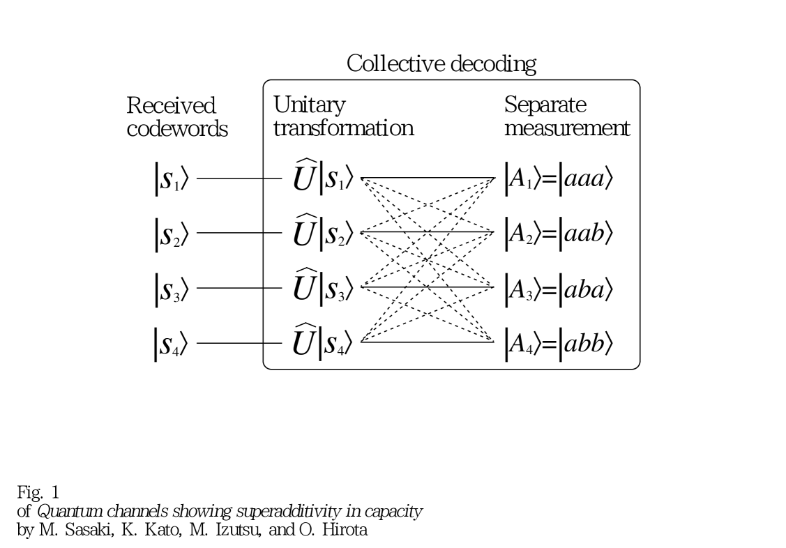
FIG. 1.: The channel model obtained by decomposing the collective decoding into the unitary transformation and the separate measurement in the case of $n=3$ and $M=4$.

FIG. 2.: The difference between the mutual information per letter state $I_{n}(S:\mu)/n$ and $C_{1}(\hat{\bf s})$ for $n=2\sim 13$

. The dashed line corresponds to the case of $n=2$, while the solid lines correspond to the case of $n=3\sim 13$.

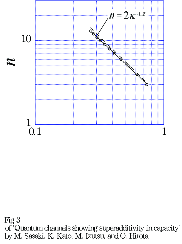
FIG. 3.: The relation between $n$ and $\kappa_{\ast}$ $(<1)$ at which $I_{n}(S:\mu)/n=C_{1}(\hat{\bf s})$ holds. $\kappa_{\ast}$’s are denoted by the circles. The solid line is just a guide for eye. The dashed line corresponding to the curve of $n=2\kappa^{-1.5}$.

FIG. 4.: $C(\hat{\bf s})$, $I_{9}(S:\mu)/9$ and $C_{1}(\hat{\bf s})$ as functions of $\kappa$.

FIG. 5.: The minimum average error probabilities corresponding to the code $[[n,n-1,2]]$ (solid lines), the initial channel, i.e., $p$ (dashed line), and the threshold points (dotted lines) as functions of $\kappa$.

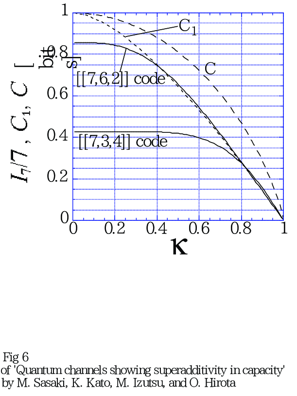
FIG. 6.: $C(\hat{\bf s})$, $I_{7}(S:\mu)/7$ for both of the [[7,3,4]] simplex code and the [[7,6,2]] code, and $C_{1}(\hat{\bf s})$ as functions of $\kappa$.

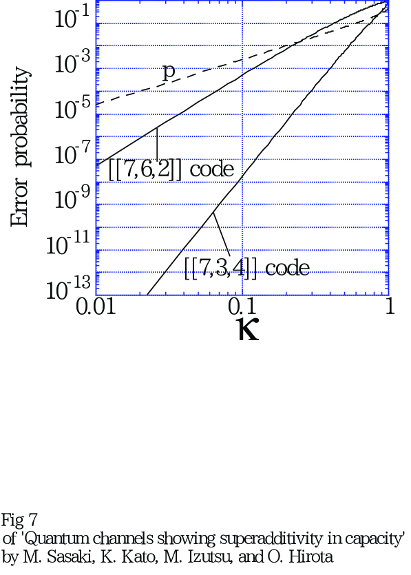
FIG. 7.: The minimum average error probabilities corresponding to the [[7,3,4]] simplex code, the [[7,6,2]] code , and the initial channel, i.e., $p$ (dashed line) as functions of $\kappa$.

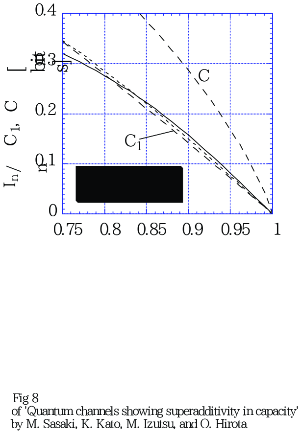
FIG. 8.: The mutual informations per letter corresponding to the [[7,3,4]] simplex code (solid line) and the code [[3,2,2]] (dashed line) as functions of $\kappa$.

REFERENCES

• [1] A. S. Holevo, Probl. Peredachi Inform. vol 9, no. 3, 3111 (1973).
• [2] A. S. Holevo, Probl. Peredachi Inform. vol 15, no. 4, 3 (1979).
• [3] P. Hausladen, R. Jozsa, B. Schumacher, M. Westmoreland and W. K. Wootters, Phys. Rev. A54, 1869 (1996).
• [4] A. S. Holevo, Report No. quant-ph/9611023, Nov. to appear in IEEE Trans. IT.
• [5] B. Schumacher and M. Westmoreland, Phys. Rev. A56, 131 (1997).
• [6] A. S. Holevo, Report No. quant-ph/9708046, 27 Aug. (1997).
• [7] C. W. Helstrom : Quantum Detection and Estimation Theory (Academic Press, New York, 1976).
• [8] A. S. Holevo, Theory Prob. Appl., vol. 23, 411, June(1978).
• [9] P. Hausladen and W. K. Wootters, J. Mod. Opt. 41, 2385 (1994).
• [10] C. A. Fuchs and A. Peres, Phys. Rev. A53, 2038 (1996)
• [11] M. Ban, K. Yamazaki, and O. Hirota, Phys. Rev. A55, 22 (1997).
• [12] M. Osaki, M. Ban, and O. Hirota, to appear in J. Mod. Opt. (1997).
• [13] A. S. Holevo, J. Multivar. Anal. 3, 337, (1973).
• [14] M. Osaki and O. Hirota, Quantum Communication and Measurement, pp401-409, ( ed. by Belavkin, Hirota, and Hudson, Plenum Publishing, New York, 1995); M. Osaki, M. Ban, and O. Hirota, Phys. Rev. A54, 1691, (1996).
• [15] C. W. Helstrom, IEEE Trans., IT-28, 359, (1982).
• [16] M. Ban, K. Kurokawa, R. Momose, and O. Hirota, Inter. J. Theor. Phys. 36, 1269 (1997).
• [17] O. Hirota, Opt. Commun., 67, 204, (1988).
• [18] M. Sasaki and O. Hirota: Phys. Lett. A210, 21 (1996); ibidA224, 213 (1997); M. Sasaki, T. S. Usuda, and O. Hirota, A. S. Holevo, Phys. Rev. A53, 1273, (1996); M. Sasaki and O. Hirota, ibid54, 2728, (1996).
• [19] A. Barenco, C. H. Bennett, R. Cleve, D. P. M. DiVincenzo, N. Margolus, P. Shor, T. Sleator, J. A. Smolin, and H. Weinfurter, Phys. Rev. A52, 3457, (1995).
• [20] M. Reck, A. Zeilinger, H. J. Bernstein, and P. Bertani, Phys. Rev. Lett. 73, 58 (1994).
• [21] T. Sleator and H. Weinfurter, Phys. Rev. Lett. 74, 4087 (1995).
• [22] Q. A. Turchette, C. J. Hood, W. Lange, H. Mabuchi, and H. J. Kimble, Phys. Rev. Lett. 75, 4710 (1995).
• [23] The authors are indebted to a private communication from A. S. Holevo for the proofs of Theorem 2 and 3.
• [24] M. Sasaki, K. Kato, M. Izutsu, and O. Hirota, to appear in Phys. Lett. A (1997).
Refer to caption