FAULT-TOLERANT QUANTUM COMPUTATION

Abstract

The discovery of quantum error correction has greatly improved the long-term prospects for quantum computing technology. Encoded quantum information can be protected from errors that arise due to uncontrolled interactions with the environment, or due to imperfect implementations of quantum logical operations. Recovery from errors can work effectively even if occasional mistakes occur during the recovery procedure. Furthermore, encoded quantum information can be processed without serious propagation of errors. In principle, an arbitrarily long quantum computation can be performed reliably, provided that the average probability of error per quantum gate is less than a certain critical value, the accuracy threshold. It may be possible to incorporate intrinsic fault tolerance into the design of quantum computing hardware, perhaps by invoking topological Aharonov-Bohm interactions to process quantum information.

1 The need for fault tolerance

Quantum computers appear to be capable, at least in principle, of solving certain problems far faster than any conceivable classical computer.[1]${}^{\!-\,}$[3] In practice, though, quantum computing technology is still in its infancy. While a practical and useful quantum computer may eventually be constructed, we cannot clearly envision at present what the hardware of that machine will be like. Nevertheless, we can be quite confident that any practical quantum computer will incorporate some type of error correction into its operation. Quantum computers are far more susceptible to making errors than conventional digital computers, and some method of controlling and correcting those errors will be needed to prevent a quantum computer from crashing.

The most formidable enemy of the quantum computer is decoherence.[4]${}^{\!-\,}$[8] We know how to prepare a quantum state of a cat that is a superposition of a dead cat and a live cat, but we never observe such macroscopic superpositions because they are very unstable. No real cat can be perfectly isolated from its environment. The environment measures the cat, in effect, immediately projecting it onto a state that is completely alive or completely dead.[9] A quantum computer may not be as complex as a cat, but it is a complicated quantum system, and like a cat it inevitably interacts with the environment. The information stored in the computer decays, resulting in errors and the failure of the computation. Can we protect a quantum computer from the debilitating effects of decoherence?

And decoherence is not our only enemy.[4]${}^{\!-\,}$[6] Even if we were able to achieve excellent isolation of our computer from the environment, we could not expect to execute quantum logic gates with perfect accuracy. As with an analog classical computer, the errors in the quantum gates form a continuum. Small errors in the gates can accumulate over the course of a computation, eventually causing failure, and it is not obvious how to correct these small errors. Can we prevent the catastrophic accumulation of the small gate errors?

The future prospects for quantum computing received a tremendous boost from the discovery[10]${}^{\!-\,}$[12] that quantum error correction is really possible in principle (see the preceding chapter by A. Steane). But this discovery in itself is not sufficient to ensure that a noisy quantum computer can perform reliably. To carry out a quantum error-correction protocol, we must first encode the quantum information we want to protect, and then repeatedly perform recovery operations that reverse the errors that accumulate. But encoding and recovery are themselves complex quantum computations, and errors will inevitably occur while we perform these operations. Thus, we need to find methods for recovering from errors that are sufficiently robust to succeed with high reliability even when we make some errors during the recovery step.

Furthermore, to operate a quantum computer, we must do more than just store quantum information; we must process the information. We need to be able to perform quantum gates, in which two or more encoded qubits come together and interact with one another. If an error occurs in one qubit, and then that qubit interacts with another through the operation of a quantum gate, the error is likely to spread to the second qubit. We must design our gates to minimize the propagation of error.

Incorporating quantum error correction will surely complicate the operation of a quantum computer. To establish the redundancy needed to protect against errors, the number of elementary qubits will have to rise. Performing gates on encoded information, and inserting periodic error-recovery steps, will slow the computation down. Because of this necessary increase in the complexity of the device, it is not a priori obvious that error correction will really improve its performance.

A device that works effectively even when its elementary components are imperfect is said to be fault tolerant. This chapter is devoted to the theory of fault-tolerant quantum computation. We will address the issues and questions summarized above.

In fact, similar issues also arise in the theory of fault-tolerant classical computation. Because existing silicon-based circuitry is so remarkably reliable, fault-tolerance is not essential to the operation of modern digital computers. Even so, the study of fault-tolerant classical computing has a distinguished history. In 1952, Von Neumann [13] suggested improving the reliability of a circuit with noisy gates by executing each gate many times, and using majority voting. He concluded that if the gate failures are statistically independent, and the probability of failure per gate is small enough, then any computation can be performed with reasonable reliability. One shortcoming of Von Neumann’s analysis was that he assumed perfect transmission of bits through the “wires” connecting the gates. Going beyond this assumption proved difficult, but was eventually achieved in 1983 by Gács,[14] who described a universal cellular automaton with a hierarchical organization that can be maintained by local operations in the presence of noise, without any need for direct nonlocal communication among the components.

It is an interesting question whether a quantum system can similarly maintain a complex hierarchical structure, but we will not be so ambitious as to address this question here. Because we are interested in the limitations imposed by noise on the processing of quantum information, we will classify our gates into classical and quantum, and we will assume that the classical gates can be executed with perfect accuracy and as quickly as necessary. This assumption will be well justified as long as the clock speed and accuracy of our classical computer far exceed those of the quantum computer.

After reviewing the features of a particular quantum error-correcting code (Steane’s 7-qubit code[12]) in §2, we assemble the ingredients of fault-tolerant recovery in §3. Errors that occur during recovery can further damage the encoded quantum information; hence recovery must be implemented carefully to be effective. Ancilla qubits are used to measure an error syndrome that diagnoses the errors in the encoded data block, and we must minimize the propagation of errors from the ancilla to the data. Methods for controlling error propagation during recovery (proposed by Peter Shor[15] and Andrew Steane[16]) are described.

Fault-tolerant processing of quantum information is the subject of §4. The central challenge is to construct a universal set of quantum gates that can act on the encoded data blocks without introducing an excessive number of errors. Some schemes for universal computation (due to Peter Shor[15] and Daniel Gottesman[17]) are outlined.

Once the elementary gates of our quantum computer are sufficiently reliable, we can perform fault-tolerant quantum gates on encoded information, along with fault-tolerant error recovery, to improve the reliability of the device. But for any fixed quantum code, or even for most infinite classes that contain codes of arbitrarily large block size, these procedures will eventually fail if we attempt a very long computation. However, it is shown in §5 that there is a special class of codes (concatenated codes) which enable us to perform longer and longer quantum computations reliably, as we increase the block size at a modest rate.[18]${}^{\!-\,}$[24] Invoking concatenated codes we can establish an accuracy threshold for quantum computation; once our hardware meets a specified standard of accuracy, quantum error-correcting codes and fault-tolerant procedures enable us to perform arbitrarily long quantum computations with arbitrarily high reliability. This result is roughly analogous to Von Neumann’s conclusion regarding classical fault-tolerance, while the hierarchical structure of concatenated coding is reminiscent of the Gács construction. We outline an estimate of the accuracy threshold, given assumptions about the errors that are enumerated in §6.

With the development of fault tolerant methods, we now know that it is possible in principle for the operator of a quantum computer to actively intervene to stabilize the device against errors in a noisy (but not too noisy) environment. In the long term, though, fault tolerance might be achieved in practical quantum computers by a rather different route—with intrinsically fault-tolerant hardware. Such hardware, designed to be impervious to localized influences, could be operated relatively carelessly, yet could still store and process quantum information robustly. The topic of §7 is a scheme for fault-tolerant hardware envisioned by Alexei Kitaev,[25] in which the quantum gates exploit nonabelian Aharonov-Bohm interactions among distantly separated quasiparticles in a suitably constructed two-dimensional spin system. Though the laboratory implementation of Kitaev’s idea may be far in the future, his work offers a new slant on quantum fault tolerance that shuns the analysis of abstract quantum circuits, in favor of new physics principles that might be exploited in the reliable processing of quantum information.

The claims made in this chapter about the potential for the fault-tolerant manipulation of complex quantum states may seem grandiose from the perspective of present-day technology. Surely, we have far to go before devices are constructed that can, say, exploit the accuracy threshold for quantum computation. Nevertheless, I feel strongly that recent work relating to quantum error correction will have an enduring legacy. Theoretical quantum computation has developed at a spectacular pace over the past three years. If, as appears to be the case, the quantum classification of computational complexity differs from the classical classification, then no conceivable classical computer can accurately predict the behavior of even a modest number of qubits (of order 100). Perhaps, then, relatively small quantum systems will have far greater potential than we now suspect to surprise, baffle, and delight us. Yet this potential could never be realized were we unable to protect such systems from the destructive effects of noise and decoherence. Thus the discovery of fault-tolerant methods for quantum error recovery and quantum computation has exceptionally deep implications, both for the future of experimental physics and for the future of technology. The theoretical advances have illuminated the path toward a future in which intricate quantum systems may be persuaded to do our bidding.

2 Quantum error correction: the 7-qubit code

To see how quantum error correction is possible, it is very instructive to study a particular code. A simple and important example of a quantum error-correcting code is the 7-qubit code devised by Andrew Steane. [11, 12] This code enables us to store one qubit of quantum information (an arbitrary state in a two-dimensional Hilbert space) using altogether 7-qubits (by embedding the two-dimensional Hilbert space in a space of dimension $2^{7}$). Steane’s code is actually closely related to a familiar classical error-correcting code, the [7,4,3] Hamming code. [26] To understand why Steane’s code works, it is important to first understand the classical Hamming code.

The Hamming code uses a block of 7 bits to encode 4 bits of classical information; that is, there are $16=2^{4}$ strings of length 7 that are the valid codewords. The codewords can be characterized by a parity check matrix

$$H=\pmatrix{0&0&0&1&1&1&1\cr 0&1&1&0&0&1&1\cr 1&0&1&0&1&0&1\cr}\ .$$ (1)

Each valid codeword is a 7-bit string $v_{\rm code}$ that satisfies

$$\sum_{k}H_{jk}\left(v_{{\rm code}}\right)_{k}=0~{}({\rm mod~{}2})\ ;$$ (2)

that is, the matrix $H$ annihilates each codeword in mod 2 arithmetic. Since $Z_{2}=\{0,1\}$ is a (finite) field, familiar results of linear algebra apply here. $H$ has three linearly independent rows and its kernel is spanned by four linearly independent column vectors. The 16 valid codewords are obtained by taking all possible linear combinations of these four strings, with coefficients chosen from $\{0,1\}$.

Now suppose that $v_{\rm code}$ is an (unknown) valid codeword, and that a single (unknown) error occurs: one of the seven bits flips. We are assigned the task of determining which bit flipped, so that the error can be corrected. This trick can be performed by applying the parity check matrix to the string. Let $e_{i}$ denote the string with a one in the $i$th place, and zeros elsewhere. Then when the $i$th bit flips, $v_{\rm code}$ becomes $v_{\rm code}+e_{i}$. If we apply $H$ to this string we obtain

$$H\left(v_{\rm code}+e_{i}\right)=He_{i}$$ (3)

(because $H$ annihilates $v_{\rm code}$), which is just the $i$th column of the matrix $H$. Since all of the columns of $H$ are distinct, we can infer $i$; we have learned where the error occurred, and we can correct the error by flipping the $i$th bit back. Thus, we can recover the encoded data unambiguously if only one bit flips; but if two or more different bits flip, the encoded data will be damaged. It is noteworthy that the quantity $He_{i}$ reveals the location of the error without telling us anything about $v_{\rm code}$; that is, without revealing the encoded information.

Steane’s code generalizes this sort of classical error-correcting code to a quantum error-correcting code. The code uses a 7-qubit “block” to encode one qubit of quantum information, that is, we can encode an arbitrary state in a two-dimensional Hilbert space spanned by two states: the “logical zero” $|0\rangle_{\rm code}$ and the “logical one” $|1\rangle_{\rm code}$. The code is designed to enable us to recover from an arbitrary error occurring in any of the 7 qubits in the block.

What do we mean by an arbitrary error? The qubit in question might undergo a random unitary transformation, or it might decohere by becoming entangled with states of the environment. Suppose that, if no error occurs, the qubit ought be in the state $a|0\rangle+b|1\rangle$. (Of course, this particular qubit might be entangled with others, so the coefficients $a$ and $b$ need not be complex numbers; they can be states that are orthogonal to both $|0\rangle$ and $|1\rangle$, which we assume are unaffected by the error.) Now if the qubit is afflicted by an arbitrary error, the resulting state can be expanded in the form:

$$a|0\rangle+b|1\rangle\longrightarrow \left(a|0\rangle+b|1\rangle\right) \otimes\quad|A_{\rm no~{}error}~{}~{}~{}\rangle_{\rm env}$$

$$+ \left(a|1\rangle+b|0\rangle\right) \otimes\quad|A_{\rm bit-flip}~{}~{}~{}~{}\rangle_{\rm env}$$

$$+ \left(a|0\rangle-b|1\rangle\right) \otimes\quad|A_{\rm phase-flip}~{}\rangle_{\rm env}$$

$$+ \left(a|1\rangle-b|0\rangle\right) \otimes\quad|A_{\rm both~{}errors}\rangle_{\rm env}\ ,$$

where each $|A\rangle_{\rm env}$ denotes a state of the environment. We are making no particular assumption about the orthogonality or normalization of the $|A\rangle_{\rm env}$ states, so Eq. (2) entails no loss of generality. We conclude that the evolution of the qubit can be expressed as a linear combination of four possibilities: (1) no error occurs, (2) the bit flip $|0\rangle\leftrightarrow|1\rangle$ occurs, (3) the relative phase of $|0\rangle$ and $|1\rangle$ flips, (4) both a bit flip and a phase flip occur.

Now it is clear how a quantum error-correcting code should work.[12, 27] By making a suitable measurement, we wish to diagnose which of these four possibilities actually occurred. Of course, in general, the state of the qubit will be a linear combination of these four states, but the measurement should project the state onto the basis used in Eq. (2). We can then proceed to correct the error by applying one of the four unitary transformations:

$$(1)~{}{\bf 1}\ ,\quad(2)~{}X\equiv\pmatrix{0&1\cr 1&0\cr}\ ,\quad(3)~{}Z\equiv\pmatrix{1&0\cr 0&-1\cr}\ ,\quad(4)~{}Y\equiv X\cdot Z\ ,$$ (5)

(and the measurement outcome will tell us which one to apply). By applying this transformation, we restore the qubit to its intended value, and completely disentangle the quantum state of the qubit from the state of the environment. It is essential, though, that in diagnosing the error, we learn nothing about the encoded quantum information, for to find out anything about the coefficients $a$ and $b$ in Eq. (2) would necessarily destroy the coherence of the qubit.

Figure 1: Diagrammatic notation for the NOT gate, the XOR (controlled-NOT) gate, and the Toffoli (controlled-controlled-NOT) gate.

Figure 2: Computation of the bit-flip syndrome for Steane’s 7-qubit code. Repeating the computation in the rotated basis diagnoses the phase-flip errors. To make the procedure fault tolerant, each ancilla qubit must be replaced by four qubits in a suitable state.

If we use Steane’s code, a measurement meeting these criteria is possible. The logical zero is the equally weighted superposition of all of the even weight codewords of the Hamming code (those with an even number of 1’s),

$$|0\rangle_{\rm code} = {1\over\sqrt{8}}\left(\sum_{{\rm even}~{}v\atop\in~{}{\rm Hamming}}|v\rangle\right)$$

$$={1\over\sqrt{8}} \Big{(}|0000000\rangle+|0001111\rangle+|0110011\rangle+|0111100\rangle$$

$$+|1010101\rangle+|1011010\rangle+|1100110\rangle+|1101001\rangle\Big{)}\ ,$$

and the logical 1 is the equally weighted superposition of all of the odd weight codewords of the Hamming code (those with an odd number of 1’s),

$$|1\rangle_{\rm code} = {1\over\sqrt{8}}\left(\sum_{{\rm odd}~{}v\atop\in~{}{\rm Hamming}}|v\rangle\right)$$

$$={1\over\sqrt{8}} \Big{(}|1111111\rangle+|1110000\rangle+|1001100\rangle+|1000011\rangle$$

$$+|0101010\rangle+|0100101\rangle+|0011001\rangle+|0010110\rangle\Big{)}\ .$$

Since all of the states appearing in Eq. (2) and Eq. (2) are Hamming codewords, it is easy to detect a single bit flip in the block by doing a simple quantum computation, as illustrated in Fig. 2 (using notation defined in Fig 1). We augment the block of 7 qubits with 3 ancilla bits, and perform the unitary operation:

$$|v\rangle\otimes|0\rangle_{\rm anc}\longrightarrow|v\rangle\otimes|Hv\rangle_{\rm anc}\ ,$$ (8)

where $H$ is the Hamming parity check matrix, and $|\cdot\rangle_{\rm anc}$ denotes the state of the three ancilla bits. If we assume that only a single one of the 7 qubits in the block is in error, measuring the ancilla projects that qubit onto either a state with a bit flip or a state with no flip (rather than any nontrivial superposition of the two). If the bit does flip, the measurement outcome diagnoses which bit was affected, without revealing anything about the quantum information encoded in the block.

But to perform quantum error correction, we will need to diagnose phase errors as well as bit flip errors. To accomplish this, we observe (following Steane[11, 12]) that we can change the basis for each qubit by applying the Hadamard rotation

$$R={1\over\sqrt{2}}\pmatrix{1&1\cr 1&-1\cr}\ .$$ (9)

Then phase errors in the $|0\rangle$, $|1\rangle$ basis become bit flip errors in the rotated basis

$$|\tilde{0}\rangle\equiv{1\over\sqrt{2}}\left(|0\rangle+|1\rangle\right)\ ,\quad|\tilde{1}\rangle\equiv{1\over\sqrt{2}}\left(|0\rangle-|1\rangle\right)\ .$$ (10)

It will therefore be sufficient if our code is able to diagnose bit flip errors in this rotated basis. But if we apply the Hadamard rotation to each of the 7 qubits, then Steane’s logical 0 and logical 1 become in the rotated basis

$$|\tilde{0}\rangle_{\rm code}= {1\over 4}\left(\sum_{v\in\atop{\rm Hamming}}|v\rangle\right)={1\over\sqrt{2}}\left(|0\rangle_{\rm code}+|1\rangle_{\rm code}\right)\ ,$$

$$|\tilde{1}\rangle_{\rm code}= {1\over 4}\left(\sum_{v\in\atop{\rm Hamming}}(-1)^{wt(v)}|v\rangle\right)={1\over\sqrt{2}}\left(|0\rangle_{\rm code}-|1\rangle_{\rm code}\right)\$$

(where $wt(v)$ denotes the weight of $v$). The key point is that $|\tilde{0}\rangle_{\rm code}$ and $|\tilde{1}\rangle_{\rm code}$, like $|0\rangle_{\rm code}$ and $|1\rangle_{\rm code}$, are superpositions of Hamming codewords. Hence, in the rotated basis, as in the original basis, we can perform the Hamming parity check to diagnose bit flips, which are phase flips in the original basis. Assuming that only one qubit is in error, performing the parity check in both bases completely diagnoses the error, and enables us to correct it.

In the above description of the error correction scheme, I assumed that the error affected only one of the qubits in the block. Clearly, this assumption as stated is not realistic; all of the qubits will typically become entangled with the environment to some degree. However, as we have seen, the procedure for determining the error syndrome will typically project each qubit onto a state in which no error has occurred. For each qubit, there is a non-zero probability of an error, assumed small, which we’ll call $\epsilon$. Now we will make a very important assumption – that the errors acting on different qubits in the same block are completely uncorrelated with one another. Under this assumption, the probability of two errors is of order $\epsilon^{2}$, and so is much smaller than the probability of a single error if $\epsilon$ is small enough. So, to order $\epsilon$ accuracy, we can safely confine our attention to the case where at most one qubit per block is in error. (In fact, to reach this conclusion, we do not really require that errors acting on different qubits be completely uncorrelated. If all qubits are exposed to the same weak magnetic field, so that each has a probability $\epsilon$ of flipping over, that would be okay because the probability that two spins flip over is order $\epsilon^{2}$. What would cause trouble is a process occuring with probability of order $\epsilon$ that flips two spins at once.)

But in the (unlikely) event of two errors occurring in the same block of the code, our recovery procedure will typically fail. If two bits flip in the same block, then the Hamming parity check will misdiagnose the error. Recovery will restore the quantum state to the code subspace, but the encoded information in the block will undergo the bit flip

$$|0\rangle_{\rm code}\rightarrow|1\rangle_{\rm code}\ ,\quad|1\rangle_{\rm code}\rightarrow|0\rangle_{\rm code}\ .$$ (12)

Similarly, if there are two phase errors in the same block, these are two bit flip errors in the rotated basis, so that after recovery the block will have undergone a bit flip in the rotated basis, or in the original basis the phase flip

$$|0\rangle_{\rm code}\rightarrow|0\rangle_{\rm code}\ ,\quad|1\rangle_{\rm code}\rightarrow-|1\rangle_{\rm code}\ .$$ (13)

(If one qubit in the block has a phase error, and another one has a bit flip error, then recovery will be successful.)

Thus we have seen that Steane’s code can enhance the reliability of stored quantum information. Suppose that we want to store one qubit in an unknown pure state $|\psi\rangle$. Due to imperfections in our storage device, the state $\rho_{\rm out}$ that we recover will have suffered a loss of fidelity:

$$F\equiv\langle\psi|\rho_{\rm out}|\psi\rangle=1-\epsilon\ .$$ (14)

But if we store the qubit using Steane’s 7-qubit block code, if each of the 7-qubits is maintained with fidelity $F=1-\epsilon$, if the errors on the qubits are uncorrelated, and if we can perform error recovery, encoding, and decoding flawlessly (more on this below), then the encoded information can be maintained with an improved fidelity $F=1-O\left(\epsilon^{2}\right)$.

Figure 3: An encoding circuit for Steane’s 7-qubit code.

A qubit in an unknown state can be encoded using the circuit shown in Fig. 3. It is easiest to understand how the encoder works by using an alternative expression for the Hamming parity check matrix,

$$H=\pmatrix{1&0&0&1&0&1&1\cr 0&1&0&1&1&0&1\cr 0&0&1&1&1&1&0\cr}\ .$$ (15)

(This form of $H$ is obtained from the form in Eq. (1) by permuting the columns, which is just a relabeling of the bits in the block.) The even subcode of the Hamming code is actually the space spanned by the rows of $H$; so we see that (in this representation of $H$) the first three bits of the string completely characterize the data represented in the subcode. The remaining four bits are the parity bits that provide the redundancy needed to protect against errors. When encoding the unknown state $a|0\rangle+b|1\rangle$, the encoder first uses two XOR’s to prepare the state $a|0000000\rangle+b|0000111\rangle$, a superposition of even and odd Hamming codewords. The rest of the circuit adds $|0\rangle_{\rm code}$ to this state: the Hadamard ($R$) rotations prepare an equally weighted superposition of all eight possible values for the first three bits in the block, and the remaining XOR gates switch on the parity bits dictated by $H$.

We will also want to be able to measure the encoded qubit, say by projecting onto the orthogonal basis $\{|0\rangle_{\rm code},|1\rangle_{\rm code}\}$. If we don’t mind destroying the encoded block when we make the measurement, then it is sufficient to measure each of the seven qubits in the block by projecting onto the basis $\{|0\rangle,|1\rangle\}$; we then perform classical error correction on the measurement outcomes to obtain a Hamming codeword. The parity of that codeword is the value of the logical qubit. (The classical error correction step provides protection against measurement errors. For example, if the block is in the state $|0\rangle_{\rm code}$, then two independent errors would have to occur in the measurement of the elementary qubits for the measurement of the logical qubit to yield the incorrect value $|1\rangle_{\rm code}$.)

In applications to quantum computation, we will need to perform a measurement that projects onto $\{|0\rangle_{\rm code},|1\rangle_{\rm code}\}$ without destroying the block. This task is accomplished by copying the parity of the block onto an ancilla qubit, and then measuring the ancilla. A circuit that performs a nondestructive measurement of the code block (in the case where the parity check matrix is as in Eq. (15)) is shown in Fig. 4. The measurement is nondestructive in the sense that it preserves the code subspace; it does, of course “destroy” a coherent superposition $a|0\rangle_{\rm code}+b|1\rangle_{\rm code}$ by collapsing the state to either $|0\rangle_{\rm code}$ (with probability $|a|^{2}$) or $|1\rangle_{\rm code}$ (with probability $|b|^{2}$).

Figure 4: Destructive and nondestructive measurement of the logical qubit.

Steane’s 7-qubit code can recover from only a single error in the code block, but better codes can be constructed[12]${}^{\!,\,}$[28]${}^{\!-\,}$[31] that can protect the information from up to $t$ errors within a single block, so that the encoded information can be maintained with a fidelity $F=1-O\left(\epsilon^{t+1}\right)$. The current status of quantum coding theory is reviewed by Steane in this volume.

The key conceptual insight that makes quantum error correction possible is that we can fight entanglement with entanglement. Entanglement can be our enemy, since entanglement of our device with the environment can conceal quantum information from us, and so cause errors. But entanglement can also be our friend—we can encode the information that we want to protect in entanglement, that is, in correlations involving a large number of qubits. This information, then, cannot be accessed if we measure just a few qubits. By the same token, the information cannot be damaged if the environment interacts with just a few qubits.

Furthermore, we have learned that, although the quantum computer is in a sense an analog device, we can digitalize the errors that it makes. We deal with small errors by making appropriate measurements that project the state of our quantum computer onto either a state where no error has occurred, or a state with a large error, which can then be corrected with familiar methods. And we have seen that it is possible to measure the errors without measuring the data—we can acquire information about the precise nature of the error without acquiring any information about the quantum information encoded in our device (which would result in decoherence and failure of our computation).

All quantum error correcting codes make use of the same fundamental strategy: a small subspace of the Hilbert space of our device is designated as the code subspace. This space is carefully chosen so that all of the errors that we want to correct move the code space to mutually orthogonal error subspaces. We can make a measurement after our system has interacted with the environment that tells us in which of these mutually orthogonal subspaces the system resides, and hence infer exactly what type of error occurred. The error can then be repaired by applying an appropriate unitary transformation.

3 Fault-tolerant recovery

In our discussion so far, we have assumed that we can encode quantum information and perform recovery from errors without making any mistakes. But, of course, error recovery will not be flawless. Recovery is itself a quantum computation that will be prone to error. If the probability of error for each bit in our code block is $\epsilon$, then it is reasonable to suppose that each quantum gate that we employ in the recovery procedure has a probability of order $\epsilon$ of introducing an error (or that “storage errors” occur with probability of order $\epsilon$ during recovery). If our recovery procedure is carelessly designed, then the probability that the procedure fails (e.g., because two errors occur in the same block) may be of order $\epsilon$. Then we have derived no benefit from using a quantum error-correcting code; in fact, the probability of error per data qubit is even higher than without any coding. So we are obligated to consider systematically all the possible ways that recovery might fail with a probability of order $\epsilon$, and to ensure that they are all eliminated. Only then is our procedure fault tolerant, and only then is coding guaranteed to pay off once $\epsilon$ is small enough.

3.1 The Back Action Problem

One serious concern is propagation of error. If an error occurs in one qubit, and then we apply a gate in which that qubit interacts with another, the error is likely to spread to the second qubit. We need to be careful to contain the infection, or at least we must strive to prevent two errors from appearing in a single block.

In performing error recovery, we repeatedly use the two-qubit XOR gate. This gate can propagate errors in two different ways. First, it is obvious that if a bit flip error occurs in one qubit, and that qubit is then used as the source qubit of an XOR gate, then the bit flip will propagate “forward” to the target qubit. The second type of error propagation is more subtle, and can be understood using the identity represented in Fig. 5 — if we perform a rotation of basis with a Hadamard gate on both qubits, then the source and the target of the XOR gate are interchanged. Since we recall that this change of basis also interchanges a bit flip error with a phase error, we infer that if a phase error occurs in one qubit, and that qubit is then used as the target qubit of an XOR gate, then the error will propagate “backward” to the source qubit.

Figure 5: A useful identity. The source and the target of an XOR gate are interchanged if we perform a change of basis with Hadamard rotations.

We can now see that the circuit shown in Fig. 2 is not fault tolerant. The trouble is that a single ancilla qubit is used as a target for four successive XOR gates. If just a single phase error occurs in the ancilla qubit at some stage, that one error can feed back to two or more of the qubits in the data block. The result is that a block phase error may occur with a probability of order $\epsilon$, which is not acceptable.

Figure 6: Bad and good versions of syndrome measurement. The bad circuit uses the same ancilla bit several times; the good circuit uses each ancilla bit only once.

To reduce the failure probability to order $\epsilon^{2}$, we must modify the recovery circuit so that each ancilla qubit couples to no more than one qubit within the code block. One way to do this is to expand the ancilla from one bit to four, with each bit the target of a single XOR gate, as in Fig. 6. We can then measure all four ancilla bits. The bit of the syndrome that we are seeking is the parity of the four measured bits. In effect, we have copied from the data block to the ancilla some information about the error that occurred, and we read that information when we measure the ancilla.

But this procedure is still not adequate as it stands, because we have copied too much information. The circuit entangles the ancilla with the error that has occured in the data, which is good, but it also entangles the ancilla with the encoded data itself, which is bad. The measurement of the ancilla destroys the carefully prepared superposition of basis states in the expressions Eqs. (2) and (2) for $|0\rangle_{\rm code}$ and $|1\rangle_{\rm code}$. For example, suppose we are measuring the first bit of the syndrome as in Fig. 2, but with the ancilla expanded from one bit to four. In effect, then, we are measuring the last four bits of the block. If we obtain the measurement result, say, $|0000\rangle_{\rm anc}$, then we have projected $|0\rangle_{\rm code}$ to $|0000000\rangle$ and $|1\rangle_{\rm code}$ to $|1110000\rangle$; the codewords have lost all protection against phase errors.

3.2 Preparing the Ancilla

We need to modify the recovery procedure further, preserving its good features while eliminating its bad features. We want to copy onto our ancilla the information about the errors in the data block, without feeding multiple phase errors into the data, and without destroying the coherence of the data. To meet this goal, we must prepare an appropriate state of the ancilla before the error syndrome computation begins. This state is chosen so the outcome of the ancilla measurement will reveal the information about the errors without revealing anything about the state of the data.

One way to meet this criterion was suggested by Peter Shor; The Shor state that he proposed is a state of four ancilla bits that is an equally weighted superposition of all even weight strings:

$$|{\rm Shor}\rangle_{\rm anc}={1\over\sqrt{8}}\sum_{{\rm even}~{}v}|v\rangle_{\rm anc}\ .$$ (16)

To compute each bit of the syndrome, we prepare the ancilla in a Shor state, perform four XOR gates (with appropriate qubits in the data block as the sources and the four bits of the Shor state as the targets), and then measure the ancilla state.

If the syndrome bit we are computing is trivial, then the computation adds an even weight string to the Shor state, which leaves it unchanged; if the syndrome bit is nontrivial, the Shor state is transformed to the equally weighted superposition of odd weight strings. Thus, the parity of the measurement result reveals the value of the syndrome bit, but no other information about the state of the data block can be extracted from measurement — we have found a way to extract the syndrome without damaging the codewords. (The particular string of specified parity that we find in the measurement is selected at random, and has nothing to do with the state of the data block.)

There are altogether 6 syndrome bits (3 to diagnose bit-flip errors and 3 to diagnose phase-flip errors), so the syndrome measurement uses 24 ancilla bits prepared in 6 Shor states, and 24 XOR gates.

One way to obtain the phase-flip syndrome would be to first apply 7 parallel $R$ gates to the data block to rotate the basis, then to apply the XOR gates as in Fig. 2 (but with the ancilla expanded into a Shor state), and finally to apply 7 $R$ gates to rotate the data back. However, we can use the identity represented in Fig. 5 to improve this procedure. By reversing the direction of the XOR gates (that is, by using the ancilla as the source and the data as the target), we can avoid applying the $R$ gates to the data, and hence can reduce the likelihood of damaging the data with faulty gates,[24, 16] as shown in Fig. 7.

Figure 7: (a) The procedure for computing one bit of the bit-flip error syndrome, shown schematically. The Hadamard gate applied to the “cat state” completes the preparation of the Shor state, as discussed in §3.3. Both the XOR gate and the Hadamard gate in the diagram actually represent four gates performed in parallel. (b) The procedure for computing one bit of the phase-flip error syndrome, shown schematically. It is the same as (a), but applied to the data in the Hadamard rotated basis. (c) A circuit equivalent to (b), simplified by using the identity in Fig. 5.

Another way to prepare the ancilla was proposed by Andrew Steane. His 7-qubit ancilla state is the equally weighted superposition of all Hamming codewords:

$$|{\rm Steane}\rangle_{\rm anc}={1\over 4}\sum_{v\in~{}{\rm Hamming}}|v\rangle\ .$$ (17)

(This state can also be expressed as $\left(|0\rangle_{\rm code}+|1\rangle_{\rm code}\right)/\sqrt{2}$, and can be obtained by applying the bitwise Hadamard rotation to the state $|0\rangle_{\rm code}$.) To compute the bit-flip syndrome, we XOR each qubit of the data block into the corresponding qubit of the ancilla, and measure the ancilla. Applying the Hamming parity-check matrix $H$ to the classical measurement outcome, we extract the bit-flip syndrome. As with Shor’s method, this procedure “copies” the data onto the ancilla, where the state of the ancilla has been carefully chosen to ensure that only the information about the error can be read by measuring the ancilla. For example, if there is no error, the particular string that we find in the measurement is a randomly selected Hamming codeword and tells us nothing about the state of the data. The same procedure is carried out in the rotated basis to find the phase-flip syndrome. The Steane method has the advantage over the Shor procedure that only 14 ancilla bits and 14 XOR gates are needed. But it also has the disadvantage that the ancilla preparation is more complex, so that the ancilla is somewhat more prone to error.

Figure 8: Construction and verification of the Shor state. If the measurement outcome is 1, then the state is discarded and a new Shor state is prepared.

3.3 Verifying the Ancilla

As we continue with our program to sniff our all the ways in which a recovery failure could result from a single error, we notice another potential problem. Due to error propagation, a single error that occurs during the preparation of the Shor state or Steane state could cause two phase errors in this state, and these can both propagate to the data if the faulty ancilla is used for syndrome measurement. Our procedure is not yet fault tolerant.

Therefore the state of the ancilla must be tested for multiple phase errors before it is used. If it fails the test, it should be discarded, and a new ancilla state should be constructed.

One way to construct and verify the Shor state is shown in Fig. 8. The first Hadamard gate and the first three XOR gates in this circuit prepare a “cat state” $\left(|0000\rangle+|1111\rangle\right)$, a maximally entangled state of the four ancilla bits; the final four Hadamard gates rotate the cat state to the Shor state. But a single error occuring during the second or third XOR could result in two errors in the cat state (it might become $\left(|0011\rangle+|1100\rangle\right)$). These two bit-flip errors in the cat state become two phase errors in the Shor state which will feed back to cause a block phase error during syndrome measurement.

But we notice that for all the ways that a single bad gate could cause two bit-flip errors in the cat state, the first and fourth bit of the cat state will have different values. Therefore, we add the last two XOR gates to the circuit (followed by a measurement) to verify whether these two bits of the cat state agree. If verification succeeds, we can proceed with syndrome measurement secure in the knowledge that the probability of two phase errors in the Shor state is of order $\epsilon^{2}$. If verification fails, we can throw away the cat state and try again.

Of course, a single error in the preparation circuit could also result in two phase errors in the cat state and hence two bit-flip errors in the Shor state; we have made no attempt to check the Shor state for bit-flip errors. But bit-flip errors in the Shor state are much less troublesome than phase errors. Bit-flip errors cause the syndrome measurement to be faulty, but they do not feed back and damage the data.

If we use Steane’s method of syndrome measurement, we first employ the encoding circuit Fig. 3 (with the first two XOR gates eliminated) to construct $|0\rangle_{\rm code}$, and then apply a Hadamard gate to each qubit to complete the preparation of the Steane state. Again, a single error during encoding can cause two bit flip errors in $|0\rangle_{\rm code}$ which become two phase errors in the Steane state, so that verification is required. We can verify by performing a nondestructive measurement of the state to ensure that it is $|0\rangle_{\rm code}$ (up to a single bit flip) rather than $|1\rangle_{\rm code}$. Thus we prepare two blocks in the state $|0\rangle_{\rm code}$, perform a bitwise XOR from the first block to the second, and then measure the second block destructively. We can apply classical Hamming error correction to the measurement outcome, to correct one possible bit-flip error, and identify the measured block as either $|0\rangle_{\rm code}$ or $|1\rangle_{\rm code}$. If the result is $|0\rangle_{\rm code}$, then the other block has passed inspection. If the result is $|1\rangle_{\rm code}$, then we suspect that the other block is faulty, and we flip that block to fix it.

However, this verification procedure is not yet trustworthy, because it might have been the block that we measured that was actually faulty, rather than the block we were trying to check. Hence we must repeat the verification step. If the measured block yields the same result twice in a row, the check may be deemed reliable. What if we get a different result the second time? Then we don’t know whether to flip the block we are checking or to leave it alone. We could try one more time, to break the tie, but this is not really necessary; in fact, if the two verification attempts give conflicting results, it is safe to do nothing. Because the results conflict, we know that one of the measured blocks was faulty. Therefore, the probability that the block to be checked is also faulty is order $\epsilon^{2}$ and can be neglected. With this verification procedure, we have managed to construct a Steane state such that the probability of multiple phase errors (which would feed back to the data during syndrome measurement) is of order $\epsilon^{2}$.

3.4 Verifying the Syndrome

A single bit-flip error in the ancilla will result in a faulty syndrome. The error could arise because the ancilla was prepared incorrectly, or because an error occured during the syndrome computation. The latter case is especially dangerous, because a single error, occuring with a probability of order $\epsilon$, could produce a fault in both the data block and the ancilla. This might happen because a bad XOR gate causes errors in both its source and target qubits, or because an error in the data block that occured during syndrome measurement is later propagated forward to the ancilla by an XOR.

In such cases, were we to accept the faulty syndrome and act to reverse the error, we would actually introduce a second error into the data block. So our procedure is still not fully fault tolerant; a scenario arising with a probability of order $\epsilon$ can fatally damage the encoded data.

We must therefore find a way to ensure that the syndrome is more reliable. The obvious way to do this is to repeat the syndrome measurement. It is not necessary to repeat if the syndrome measurement is trivial (indicates no error); though there actually might be an error in the data that we failed to detect, we need not worry that we will make things worse, because if we accept the syndrome we will take no action. If on the other hand the syndrome indicates an error, then we measure the syndrome a second time. If we obtain the same result again, it is safe to accept the syndrome and proceed with recovery, because there is no way occuring with a probability of order $\epsilon$ to obtain the same (nontrivial) faulty syndrome twice in a row.

If the first two syndrome measurements do not agree, then we could continue to measure the syndrome until we finally obtain the same result twice in a row, a result that can be trusted. Alternatively, we could choose to do nothing, until an error is reliably detected in a future round of error correction. At least in that event we will not make things worse by compounding the error, and if there is really an error in the data, we will probably detect it next time.

(There are also other ways to increase our confidence in the syndrome. For example, instead of repeating the measurement of the entire syndrome, we could compute some additional redundant syndrome bits, and subject the computed bits to a parity check. If there is an error in the syndrome, this method will usually detect the error; thus if the parity check passes, the syndrome is likely to be correct.[32, 24]

Finally, we have assembled all the elements of a fault-tolerant error recovery procedure. If we take all the precautions described above, then recovery will fail only if two independent errors occur, so the probability of an error occurring that irrevocably damages the encoded block will be of order $\epsilon^{2}$.

A complete quantum circuit for Steane’s error correction is shown in Fig. 9. Note that both the bit-flip and phase error correction are repeated twice. The verification of the Steane states is also shown, but the encoding of these states is suppressed in the diagram.

Figure 9: The complete circuit for Steane error recovery. Encoded $|0\rangle$’s are prepared, then verified. The verified $|0\rangle$’s are used as ancillas to compute the bit-flip and phase-flip syndromes, which are both measured twice. The large circles indicate actions that are taken (conditioned on measurement outcomes) to repair the ancilla states, or in the final step, to repair the data block.

3.5 Measurement and Encoding

We will of course want to be able to measure our encoded qubits reliably. But we have already noted in §2 that destructive measurement of the code block is reliable if only one qubit in the block has a bit-flip error. If the probability of a flawed measurement is order $\epsilon$ for a single qubit, then faulty measurements of the code block occur with probability of order $\epsilon^{2}$. Fault-tolerant nondestructive measurement can also be performed, as we have already noted in our discussion (§3.3) of the verification of the Steane state. An alternative procedure would be to use the nondestructive measurement depicted in Fig. 4 without any modification. Though the ancilla is the target of three successive XOR gates, phase errors feeding back into the block are not so harmful because they cannot change $|0\rangle_{\rm code}$ to $|1\rangle_{\rm code}$ (or vice versa). However, since a single bit-flip error (in either the data block or the ancilla qubit) can cause a faulty parity measurement, the measurement must be repeated (after bit-flip error correction) to ensure accuracy to order $\epsilon^{2}$. (We eschewed this procedure in our description of the verification of the Steane state to avoid the frustration of needing error correction to prepare the ancilla for error correction!)

We will often want to prepare known encoded quantum states, such as $|0\rangle_{\rm code}$. We already discussed in §3.3 above (in connection with preparation of the Steane state), how this encoding can be performed reliably. In fact, the encoding circuit is not actually needed. Whatever the initial state of the block, (fault-tolerant) error correction will project it onto the space spanned by $\{|0\rangle_{\rm code},|1\rangle_{\rm code}\}$, and (verified) measurement will project out either $|0\rangle_{\rm code}$ or $|1\rangle_{\rm code}$. If the result $|1\rangle_{\rm code}$ is obtained, then the (bitwise) NOT operator can be applied to flip the block to the desired state $|0\rangle_{\rm code}$.

If we wish to encode an unknown quantum state, then we use the encoding circuit in Fig. 3. Again, because of error propagation, a single error during encoding may cause an encoding failure. In this case, since no measurement can verify the encoding, the fidelity of the encoded state will inevitably be $F=1-O(\epsilon)$. However, encoding may still be worthwhile, since it may enable us to preserve the state with a reasonable fidelity for a longer time than if the state had remained unencoded.

3.6 Other Codes

Both Shor’s and Steane’s scheme for fault-tolerant syndrome measurement have been described here only for the 7-qubit code, but they can be adapted to more complex codes that have the capability to recover from many errors.[33, 16] Syndrome measurement for more general codes is best described using the code stabilizer formalism. In this formalism, which is discussed in more detail in the chapter by Andrew Steane in this volume, a quantum error-correcting code is characterized as the space of simultaneous eigenstates of a set of commuting operators (the stabilizer generators). Each generator can be expressed as a product of operators that act on a single qubit, where the single-qubit operators are chosen from the set $\{I,X,Y,Z\}$ defined in Eq. (5). Each generator squares to the identity and has equal numbers of eigenvectors with eigenvalue +1 and -1, so that specifying its eigenvalue reduces the dimension of the space by half. If there are $n$ qubits in a block, and there are $n-k$ generators, then the code subspace has dimension $2^{k}$ — there are $k$ encoded qubits.

For example, Steane’s 7-qubit code is the space for which the six stabilizer generators

$$M_{1} = (IIIZZZZ)$$

$$M_{2} = (IZZIIZZ)$$

$$M_{3} = (ZIZIZIZ)$$

$$M_{4} = (IIIXXXX)$$

$$M_{5} = (IXXIIXX)$$

$$M_{6} = (XIXIXIX)$$

all have eigenvalue one. Comparing to Eq. (1), we see that the space with $M_{1}=M_{2}=M_{3}=1$ is spanned by codewords that satisfy the Hamming parity check. Recalling that a Hadamard change of basis interchanges $Z$ and $X$, we see that the space with $M_{4}=M_{5}=M_{6}=1$ is spanned by codewords that satisfy the Hamming parity check in the Hadamard-rotated basis. Indeed, the defining property of Steane’s code is that the Hamming parity check is satisfied in both bases.

The stabilizer generators are chosen so that every error operator that is to be corrected (also expressed as a product of the one-qubit operators $\{I,X,Y,Z\}$), and the product of any two distinct such error operators, anticommutes with at least one generator. Thus, every error changes the eigenvalues of some of the generators, and two independent errors always change the eigenvalues in distinct ways. This means that we obtain a complete error syndrome by measuring the eigenvalues of all the stabilizer generators.

Measuring a stabilizer generator $M$ is not difficult. First we perform an appropriate unitary change of basis on each qubit so that $M$ in the rotated basis is a product of $I$’s and $Z$’s acting on the individual qubits. (We rotate by

$$R={1\over\sqrt{2}}\pmatrix{1&1\cr 1&-1\cr}$$ (19)

for each qubit acted on by $X$ in $M$, and by

$$R^{\prime}={1\over\sqrt{2}}\pmatrix{1&i\cr i&1\cr}$$ (20)

for each qubit acted on by $Y$.) In this basis, the value of $M$ is just the parity of the bits for which $Z$’s appear. We can measure the parity (much as we did in our discussion of the 7-qubit code), by performing an XOR to the ancilla from each qubit in the block for which a $Z$ appears in $M$. Finally, we invert the change of basis. This procedure is repeated for each stabilizer generator until the entire syndrome is obtained.

We can make this procedure fault-tolerant by preparing the ancilla in a Shor state for each syndrome bit to be measured, where the number of bits in the Shor state is the weight of the corresponding stabilizer generator (the number of one-qubit operators that are not the identity). Each ancilla bit is the target of only a single XOR, so that multiple phase errors do not feed back into the data. The procedures discussed above for verifying the Shor state and the syndrome measurement can also be suitably generalized.

For complex codes that either encode many qubits or can correct many errors, this generalized Shor method uses many more ancilla qubits and many more quantum gates than are really necessary to extract an error syndrome. We can do considerably better by generalizing the Steane method. In the case of the 7-qubit code, Steane’s idea was that we can use one 7-bit ancilla to measure all of $M_{1}$, $M_{2}$, and $M_{3}$; we prepare an initial state of the ancilla that is an equally weighted superposition of all strings that satisfy the Hamming parity check (i.e, all words in the classical Hamming code), perform the appropriate XOR’s from the data block to the ancilla, measure all ancilla qubits, and finally apply the Hamming parity check to the measurement result. The three parity bits obtained are the measured eigenvalues of $M_{1}$, $M_{2}$, and $M_{3}$. The ancilla preparation has been chosen so that no other information aside from these eigenvalues can be extracted from the measurement result; hence the coherence of our quantum codewords is not damaged by the procedure.

This procedure evidently can be adapted to the simultaneous measurement of any set of operators where each can be expressed as a product of $I$’s and $Z$’s acting on the individual qubits. Given a list of $k$ such $n$-qubit operators, we obtain a matrix $H_{Z}$ with $k$ rows and $n$ columns by replacing each $I$ in the list by 0 and each $Z$ by 1. We prepare the ancilla as the equally weighted superposition of all length-$n$ strings that obey the $H_{Z}$ parity check. Proceeding with the XOR’s and the ancilla measurement (and applying $H_{Z}$ to the measurement result), we project a block of $n$ qubits onto a simultaneous eigenstate of the $n$ operators. Performing the same procedure in the Hadamard-rotated basis, we can simultaneously measure any set of operators where each is a product of $I$’s and $X$’s.

Among the stabilizer generators there also might be operators that have the form $M=\bar{Z}\bar{X}$, where $\bar{Z}$ is a product of $Z$’s acting on one set of qubits, and $\bar{X}$ is a product of $X$’s acting on another set of qubits. Since the generator $M$ must square to the identity, the number of qubits acted on by the product $Y$ of $Z$ and $X$ must be even. Hence $\bar{Z}$ and $\bar{X}$ commute, and so can be simultaneously measured by the method described above. However, this measurement would give too much information; we want to measure the product of $\bar{Z}$ and $\bar{X}$ rather than measure each separately. To make the measurement we want, we must further modify the ancilla. The ancilla should not be chosen to satisfy both the $H_{Z}$ parity check and the corresponding $H_{X}$ parity check. Rather it is prepared so that the $H_{Z}$ and $H_{X}$ parity bits are correlated — the ancilla is a sum over strings such that either both parity bits are trivial or both bits are nontrivial. After the ancilla measurement, we sum the parity of the “$\bar{Z}$ measurement” and the “$\bar{X}$ measurement” to obtain the eigenvalue of $M$. But the separate parities of the $\bar{Z}$ and $\bar{X}$ “measurements” are entirely random and actually reveal nothing about the values of $\bar{Z}$ or $\bar{X}$.

Now we can describe Steane’s method in its general form that can be applied to any stabilizer code. If $k$ logical qubits are encoded in a block of $n$ qubits, then there are $n-k$ independent stabilizer generators. With a list of these generators we associate a matrix

$$\bar{H}=\pmatrix{H_{Z}&|&H_{X}\cr}$$ (21)

that has $n-k$ rows and $2n$ columns. The positions of the 1’s in $H_{Z}$ indicate the qubits that are acted on by $Z$ in the listed generators, and the 1’s in $H_{X}$ indicate the qubits acted on by $X$; if a 1 appears in the same position in both $H_{Z}$ and $H_{X}$, then the product $Y=ZX$ acts on that qubit. A $2n$-qubit ancilla is prepared in the generalized Steane state — the equally weighted superposition of all of the strings that satisfy the $\bar{H}$ parity check. Then the quantum circuit shown in Fig. 10 is executed, the ancilla qubits are measured, and $\bar{H}$ is applied to the measurement result. The parity bits found are the eigenvalues of the stabilizer generators, which provide the complete error syndrome.

Figure 10: Circuit for Steane syndrome measurement, shown schematically. A $2n$-qubit Steane state is used to find the syndrome for an $n$-qubit data block. Each XOR gate in the diagram represents $n$ XOR gates performed in parallel.

The ancilla preparation has been designed so that no other information other than the syndrome can be extracted from the measurement result, and therefore the coherence of the quantum codewords is not damaged by the procedure. Each qubit in the code block is acted on by only two quantum gates in this procedure, the minimum necessary to detect both bit-flip and phase errors afflicting any qubit.

Finally, we note that a different strategy for performing fault-tolerant error correction was described by Kitaev.[34] He invented a family of quantum error-correcting codes such that many errors within the code block can be corrected, but only four XOR gates are needed to compute each bit of the syndrome. In this case, even if we use just a single ancilla qubit for the computation of each syndrome bit (rather than an expanded ancilla state like a Shor or Steane state), only a limited number of errors can feed back from the ancilla into the data. The code can then be chosen such that the typical number of errors fed back into the data during the syndrome computation is comfortably less than the maximum number of errors that the code can tolerate.

4 Fault-tolerant quantum gates

We have seen that coding can protect quantum information. But we want to do more than store quantum information with high fidelity; we want to operate a quantum computer that processes the information. Of course, we could decode, perform a gate, and then re-encode, but that procedure would temporarily expose the quantum information to harm. Instead, if we want our quantum computer to operate reliably, we must be able to apply quantum gates directly to the encoded data, and these gates must respect the principles of fault tolerance if catastrophic propagation of error is to be avoided.

4.1 The 7-qubit code

In fact, with Steane’s 7-qubit code, there are a number of gates that can be easily implemented. Three single-qubit gates can all be applied bitwise; that is applying these gates to each of the 7 qubits in the block implements the same gate acting on the encoded qubit. We have already seen in Eq. (2) that the Hadamard rotation $R$ acts this way. The same is true for the NOT gate (since each odd parity Hamming codeword is the complement of an even parity Hamming codeword), and the phase gate

$$P=\pmatrix{1&0\cr 0&i\cr}\ ;$$ (22)

(the odd Hamming codewords have weight $\equiv$ 3 (mod 4) and the even codewords have weight $\equiv$ 0 (mod 4), so we actually apply $P^{-1}$ bitwise to implement $P$). The XOR gate can also be implemented bitwise; that is, by XOR’ing each bit of the source block into the corresponding bit of the target block, as in Fig. 11. This works because the even codewords form a subcode, while the odd codewords are its nontrivial coset.

Figure 11: The transversal XOR gate, shown schematically. By XOR’ing each bit of the source block into the corresponding bit of the target block, we implement an XOR acting on the encoded qubits. The gate implementation is fault tolerant because each qubit in both code blocks is acted on by a single gate.

Figure 12: The measurement circuit used in the ancilla preparation step of Shor’s implementation of the Toffoli gate.

Figure 13: The fault-tolerant Toffoli gate. Each line represents a block of 7 qubits, and the gates are implemented transversally. For each measurement, the arrow points to the set of gates that is to be applied if the measurement outcome is 1; no action is taken if the outcome is 0.

Thus there are simple fault-tolerant procedures for implementing the gates NOT, $R$, $P$, and XOR. But unfortunately, these gates do not by themselves form a universal set. To be able to perform any desired unitary transformation acting on encoded data (to arbitrary precision), we will need to make a suitable addition to this set. Following Shor,[15] we will add the 3-qubit Toffoli gate, which is implemented by the procedure shown in Fig. 13.

Shor’s construction of the fault-tolerant Toffoli gate has two stages. In the first stage, three encoded ancilla blocks are prepared in a state of the form

$$|A\rangle_{\rm anc}\equiv{1\over{2}}\sum_{a=0,1}\sum_{b=0,1}|a,b,ab\rangle_{\rm anc}\ .$$ (23)

In the second stage, the ancilla interacts with three data blocks to complete the execution of the gate. First, we will describe how the ancilla is prepared. To begin with, each of three ancilla blocks are encoded in the state $|0\rangle_{\rm code}$. Bitwise Hadamard gates are applied to all three blocks to prepare the encoded state

$${1\over\sqrt{8}}\sum_{a=0,1}\sum_{b=0,1}\sum_{c=0,1}|a,b,c\rangle_{\rm anc}\ .$$ (24)

We note that this state can be expressed as

$${1\over\sqrt{2}}\left(|A\rangle_{\rm anc}+|B\rangle_{\rm anc}\right)\ ,\quad|B\rangle_{\rm anc}\equiv{\rm NOT}_{3}|A\rangle_{\rm anc}\ ,$$ (25)

where ${\rm NOT}_{3}$ denotes a NOT gate acting on the third encoded qubit. In the remainder of the ancilla preparation, the three blocks are measured in the $\{|A\rangle_{\rm anc},|B\rangle_{\rm anc}\}$ basis; if the outcome $|A\rangle_{\rm anc}$ is obtained, the preparation is complete; if $|B\rangle_{\rm anc}$ is obtained, ${\rm NOT}_{3}$ is applied to complete the procedure.

Now we must explain how the $\{|A\rangle_{\rm anc},|B\rangle_{\rm anc}\}$ measurement is carried out. Schematically, the measurement is done with the circuit shown in Fig. 12, where the $Z_{AB}$ gate (conditioned on a control bit) flips the relative phase of $|A\rangle_{\rm anc}$ and $|B\rangle_{\rm anc}$. We can see from Eqs. (23) and (25) that, in terms of the values $a$, $b$, and $c$ of the three ancilla blocks, $Z_{AB}$ applies the phase $(-1)^{ab+c}$. If the control bit is denoted $x$, then the gates we need to apply are $(-1)^{xab}$ and $(-1)^{xc}$, the product of a three-bit phase gate and a two-bit phase gate.

But a three-bit phase gate is as hard as a Toffoli gate, so we seem to be stuck. However, we can get around this impasse if the control block is chosen to be not an encoded qubit, but instead a (verified) 7-bit “cat state”

$$|{\rm cat}\rangle={1\over\sqrt{2}}\bigl{(}|0000000\rangle+|1111111\rangle\bigr{)}\ .$$ (26)

We do already know how to construct fault-tolerant two-bit and one-bit phase gates transversally. These can be promoted to the three-bit and two-bit gates that we need by simply conditioning all of the bitwise gates in the construction on the corresponding bits of the cat state. Finally, we apply the bitwise Hadamard rotation to the cat state and measure its parity to complete the execution of the measurement circuit Fig. 12. (We obtain the circuit in Fig. 13, by noting that, if the cat state is in the Hadamard rotated basis, the three-bit phase gate can be expressed as a Toffoli gate with the cat state as target; therefore one bitwise Toffoli gate is executed in our implementation of the measurement circuit.) Of course, the measurement is repeated to ensure accuracy.

Meanwhile, three data blocks have been waiting patiently for the ancilla to be ready. By applying three XOR gates and a Hadamard rotation, the state of the data and ancilla is transformed as

$$\sum_{a=0,1}\sum_{b=0,1}|a,b,ab\rangle_{\rm anc}|x,y,z\rangle_{\rm data}$$

$$\longrightarrow\sum_{a=0,1}\sum_{b=0,1}\sum_{w=0,1}(-1)^{wz}|a,b,ab\oplus z\rangle_{\rm anc}|x\oplus a,y\oplus b,w\rangle_{\rm data}\ .$$ (27)

Now each data block is measured. If the measurement outcome is 0, no action is taken, but if the measurement outcome is 1, then a particular set of gates is applied to the ancilla, as shown in Fig. 13, to complete the implementation of the Toffoli gate. Note that the original data blocks are destroyed by the procedure, and that what were initially the ancilla blocks become the new data blocks. The important thing about this construction is that all of the steps have been carefully designed to adhere to the principles of fault tolerance and minimize the propagation of error. Thus, two independent errors must occur during the procedure in order for two errors to arise in any one of the data blocks.

That the fault-tolerant gates form a discrete set is a bit of a nuisance, but it is also an unavoidable feature of any fault-tolerant scheme. It would not make sense for the fault-tolerant gates to form a continuum, for then how could we possibly avoid making an error by applying the wrong gate, a gate that differs from the intended one by a small amount? Anyway, since our fault-tolerant gates form a universal set, they suffice for approximating any desired unitary transformation to any desired accuracy.

4.2 Other codes

Shor[15] described how to generalize this fault tolerant set of gates to more complex codes that can correct more errors, and Gottesman[17, 35] has described an even more general procedure that can be applied to any of the quantum stabilizer codes.

Gottesman’s construction begins with the observation that for any stabilizer code, there are fault-tolerant implementations of the single qubit gates $X$ and $Z$ acting on each encoded qubit. For a stabilizer code with block size $n$, recall that we have already seen in §3.6 that any “error operator” $M$ (expressed as a tensor product of $n$ matrices chosen from $\{I,X,Y,Z\}$) can be written in the form $\bar{Z}\bar{X}$, and so can be uniquely represented as a binary string of length $2n$. If there are $k$ logical qubits encoded in the block, then the stabilizer of the code is generated by $n-k$ such operators. The error operators that commute with all elements of the stabilizer themselves form a group. The generators of this group are represented by binary strings of length $2n$ that are required to satisfy $n-k$ independent binary conditions; therefore, there are $n+k$ independent generators. Of these, $n-k$ are the generators of the stabilizer, but there are in addition $2k$ independent error operators that do not lie in the stabilizer, but do commute with the stabilizer. These $2k$ operators preserve the code subspace but act nontrivially on the codewords, and therefore they can be interpreted as operations that act on the encoded logical qubits.

In fact, these $2k$ operators can be chosen as the single qubit operations $\hat{Z}_{i}$ and $\hat{X}_{i}$, where $i=1,2,3,\dots,k$ labels the encoded qubits. We first note that the $n-k$ stabilizer generators can be extended to a maximal commuting set of $n$ operators; the $k$ additional operators may be identified as the $\hat{Z}_{i}$’s. We can choose the computational basis states in the code subspace to be the simultaneous eigenstates of all the $\hat{Z}_{i}$’s, with the $+1$ eigenvalue corresponding to the value $0$, and the $-1$ eigenvalue to the value $1$. Then $\hat{Z}_{i}$ flips the phase of qubit $i$. We may choose the remaining $k$ generators, denoted $\hat{X}_{i}$, which commute with the stabilizer but not with all of the $\hat{Z}_{i}$’s, to obey the relations

$$[\hat{Z}_{i},\hat{Z}_{j}]=0=[\hat{X}_{i},\hat{X}_{j}]\ ,\quad[\hat{Z}_{i},\hat{X}_{j}]=0\ ,(i\neq j)\ ,\quad\hat{Z}_{i}\hat{X}_{i}+\hat{X}_{i}\hat{Z}_{i}=0\ .$$ (29)

Since $\hat{X}_{i}$ anticommutes with $\hat{Z}_{i}$, it flips the eigenvalue of $\hat{Z}_{i}$, and hence the value of qubit $i$. All of these operations are performed by applying at most one single-qubit gate to each qubit in the block; therefore, these operations are surely fault tolerant.

We have also seen in §3.6 that it is possible to perform a fault-tolerant measurement of any error operator $\bar{Z}\bar{X}$, and so in particular to measure each $\hat{X}_{i}$, $\hat{Y}_{i}$, and $\hat{Z}_{i}$ fault tolerantly. Gottesman[17] has shown that, if it possible to perform a Toffoli gate (which is universal for the classical computations that preserve the set of computational basis states), then the single qubit gates $X$ and $Z$, together with the ability to measure $X$, $Y$, and $Z$ for any qubit, suffice for universal quantum computation. Hence, if we can show that a fault-tolerant Toffoli gate can be constructed acting on any three qubits, we will have completed the demonstration that universal fault-tolerant quantum computation is possible with any stabilizer code.

The construction of a fault-tolerant Toffoli gate is rather complicated, so it is best to organize the demonstration this way: Gottesman showed that in any stabilizer code, it is possible to apply a fault-tolerant XOR gate to any pair of qubits (whether or not the two qubits reside in the same code block). Using the XOR gate, plus the single qubit gates and measurements that we have already seen can be implemented fault-tolerantly, one can show that all of the gates needed in Shor’s construction of the Toffoli gate can be constructed. Thus, the fault-tolerant construction of the Toffoli gate can be carried out using any stabilizer code, and universal fault-tolerant quantum computation can be achieved.

While in principle any stabilizer code can be used for fault-tolerant quantum computing, some codes are better than others. For example, there is a 5-qubit code that can recover from one error[36, 37] and Gottesman[17] has exhibited a universal set of fault-tolerant gates for this code. But the gate implementation is quite complex. The 7-qubit Steane code requires a larger block, but it is much more convenient for computation.

5 The accuracy threshold for quantum computation

Quantum error-correcting codes exist that can correct $t$ errors, where $t$ can be arbitrarily large. If we use such a code and we follow the principles of fault-tolerance, then an uncorrectable error will occur only if at least $t+1$ independent errors occur in a single block before recovery is completed. So if the probability of an error occurring per quantum gate, or the probability of a storage error occurring per unit of time, is of order $\epsilon$, then the probability of an error per gate acting on encoded data will be of order $\epsilon^{t+1}$, which is much smaller if $\epsilon$ is small enough. Indeed, it may seem that by choosing a code with $t$ as large as we please we can make the probability of error per gate as small as we please, but this turns out not to be the case, at least not for most codes. The trouble is that as we increase $t$, the complexity of the code increases sharply, and the complexity of the recovery procedure correspondingly increases. Eventually we reach the point where it takes so long to perform recovery that it is likely that $t+1$ errors will accumulate in a block before we can complete the recovery step, and the ability of the code to correct errors is thus compromised.

Suppose that the number of computational steps needed to perform the syndrome measurement increases with $t$ like a power $t^{b}$. Then the probability that $t+1$ errors accumulate before the measurement is complete will behave like

$${\rm Block~{}Error~{}Probability}\sim\left(t^{b}\epsilon\right)^{t+1}\ ,$$ (30)

where $\epsilon$ is the probability of error per step. We may then choose $t$ to minimize the error probability ($t\sim e^{-1}\epsilon^{-1/b}$, assuming $t$ is large), obtaining

$${\rm Minimum~{}Block~{}Error~{}Probability}\sim\exp\left(-e^{-1}b\epsilon^{-1/b}\right)\ .$$ (31)

Thus if we hope to carry out altogether $T$ cycles of error correction without any error occurring, then our gates must have an accuracy

$$\epsilon\sim\left(\log T\right)^{-b}\ .$$ (32)

Similarly, if we hope to perform a quantum computation with altogether $T$ quantum gates, elementary gates of this prescribed accuracy are needed.

In the procedure originally described by Shor,[15] the power characterizing the complexity of the syndrome measurement is $b=4$, and somewhat smaller values of $b$ can be achieved with a better optimized procedure. The block size of the code used grows with $t$ like $t^{2}$ (for the codes that Shor considered), so when the code is chosen to optimize the error probability, the block size is of order $(\log T)^{2}$. Certainly, the scaling described by Eq. (32) is much more favorable than the accuracy $\epsilon\sim T^{-1}$ that would be required were coding not used at all. But for any given accuracy, there is a limit to how long a computation can proceed until errors become likely.

Figure 14: Concatenated coding. Each qubit in the block, when inspected at higher resolution, is itself an encoded subblock.

This limitation can be overcome by using a special kind of code, a concatenated code.[18]${}^{\!-\,}$[24] To understand the concept of a concatenated code, imagine that we are using Steane’s quantum error-correcting code that encodes a single qubit as a block of $7$ qubits. But if we look more closely at one of the $7$ qubits in the block with better resolution, we discover that it is not really a single qubit, but another block of $7$ encoded using the same Steane code as before. And when we examine one of the $7$ qubits in this block with higher resolution, we discover that it too is really a block of $7$ qubits. And so on. (See Fig. 14.) If there are all together $L$ levels to this hierarchy of concatenation, then a single qubit is actually encoded in a block of size $7^{L}$. The reason that concatenation is useful is that it enables us to recover from errors more efficiently, by dividing and conquering. With this method, the complexity of error correction does not grow so sharply as we increase the error-correcting capacity of our quantum code.

We have seen that Steane’s 7-qubit code can recover from one error. If the probability of error per qubit is $\epsilon$, the errors are uncorrelated, and recovery is fault-tolerant, then the probability of a recovery failure is of order $\epsilon^{2}$. If we concatenate the code to construct a block of size $7^{2}$, then an error occurs in the block only if two of the subblocks of size 7 fail, which occurs with a probability of order $(\epsilon^{2})^{2}$. And if we concatenate again, then an error occurs only if two subblocks of size $7^{2}$ fail, which occurs with a probability of order $((\epsilon^{2})^{2})^{2}$. If there are all together $L$ levels of concatenation, then the probability of an error is or order $(\epsilon)^{2^{L}}$, while the block size is $7^{L}$. Now, if the error rate for our fundamental gates is small enough, then we can improve the probability of an error per gate by concatenating the code. If so, we can improve the performance even more by adding another level of concatenation. And so on. This is the origin of the accuracy threshold for quantum computation: if coding reduces the probability of error significantly, then we can make the error rate arbitrarily small by adding enough levels of concatenation. But if the error rates are too high to begin with, then coding will make things worse instead of better.

To analyze this situation, we must first adopt a particular model of the errors, and I will choose the simplest possible quasi-realistic model: uncorrelated stochastic errors. In each computational time step, each qubit in the device becomes entangled with the environment as in Eq. (2), but where we assume that the four states of the environment are mutually orthogonal, and that the three “error states” have equal norms. Thus the three types of errors (bit flip, phase flip, both) are assumed to be equally likely. The total probability of error in each time step is denoted $\epsilon_{\rm store}$. In addition to these storage errors that afflict the “resting” qubits, there will also be errors that are introduced by the quantum gates themselves. For each type of gate, the probability of error each time the gate is implemented is denoted $\epsilon_{\rm gate}$ (with independent values assigned to gates of each type). If the gate acts on more than one qubit (XOR or Toffoli), correlated errors may arise. In our analysis, we make the pessimistic assumption that an error in a multi-qubit gate always damages all of the qubits on which the gate acts; e.g., a faulty XOR gate introduces errors in both the source qubit and the target qubit. This assumption (among others) is made only to keep the analysis tractable. Under more realistic assumptions, we would find that somewhat higher error rates could be tolerated.

We can analyze the efficacy of concatenated coding by constructing a set of concatenation flow equations, that describe how our error model evolves as we proceed from one level of concatenation to the next. For example, suppose we want to perform an XOR gate followed by an error recovery step on qubits encoded using the concatenated Steane code with $L$ levels of concatenation (block size $7^{L}$). The gate implementation and recovery can be described in terms of operations that act on subblocks of size $7^{L-1}$. Thus, we can derive an expression for the probability of error $\epsilon^{(L)}$ for a gate acting on the full block in terms of the probability of error for gates acting on the subblocks. This expression is one of the flow equations. In principle, we can solve the flow equations to find the error probabilities “at level $L$” in terms of the parameters of the error model for the elementary qubits. We then study how the error probabilities behave as $L$ becomes large. If all block error probabilities approach zero for $L$ large, then the elementary error probabilities are “below the threshold.” Since our elementary error model may have many parameters, the threshold is really a codimension one surface in a high-dimension space.

Steane’s method of syndrome measurement is particularly well suited for concatenated coding. All of the gates in the recovery circuit Fig. 9 can be executed transversally; if we perform the gates on the elementary qubits in the code block, then we are executing the very same gates on the encoded information in each block of size 7, each superblock of size $7\cdot 7$ and so on. Similarly, when we measure the elementary qubits in the ancilla at the conclusion of the syndrome computation, then (after applying classical Hamming error correction to the qubits), we have also measured the encoded qubit in each block of 7, and (after applying Hamming error correction to the blocks) each superblock of $7\cdot 7$, etc. We see then that the quantum data processing needed to extract a syndrome can be carried out at all levels of the concatenated code simultaneously. After some relatively straightforward classical processing, we determine what single qubit gates need to be applied to all the elementary qubits in order to complete the recovery step on all levels at once.

Thus it is easy to see (at least conceptually) how the accuracy threshold can be estimated.[38] At each level of the concatenated code, a block of 7 fails if there are errors in at least two of the subblocks that it contains. If $p_{L}$ is the probability of an error in a block at level $L$, then the probability of an error in a block at level $L+1$ is

$$p_{L+1}\sim\left({7\atop 2}\right)p_{L}^{2}+\cdots=21~{}p_{L}^{2}+\cdots$$ (33)

(neglecting the terms of higher order in $p_{L}$), which will be smaller than $p_{L}$ if $p_{L}<1/21$. Therefore, if the each elementary qubit has a probability of error $p_{0}<1/21$, the error probability will be smaller at level 1, still smaller at level 2, and so on—the threshold value of $p_{0}$ is $1/21$.

Suppose that we perform error correction every time we execute an XOR or single qubit gate. Roughly speaking, $p_{0}$ is the probability of error per data qubit when a cycle of error correction begins. To estimate the accuracy threshold, we follow the circuit Fig. 9 and add up the contributions to $p_{0}$ due to errors (including possible storage errors) that arose during recently executed quantum gates and that have not already been eliminated in a previous error correction cycle. We obtain an expression for $p_{0}$ in terms of the gate error and storage error probabilities that we can equate to $1/21$ to find the threshold.

Proceeding this way, assuming that storage errors are negligible, and that each single-qubit or XOR gate has the same error probability $\epsilon_{\rm gate}$, we[38] crudely estimate the threshold gate error rate as

$$\epsilon_{\rm gate,0}\sim 6\cdot 10^{-4}\ .$$ (34)

Similarly, if gate errors are negligible, the estimated threshold storage error rate is

$$\epsilon_{\rm store,0}\sim 6\cdot 10^{-4}\ .$$ (35)

The thresholds for gate and storage errors are essentially the same because the Steane method is well optimized for dealing with storage errors. The qubits are rarely idle; a gate acts on each one in almost every step. Hence, the storage accuracy requirement is considerably less stringent than in previous threshold estimates based on the Shor recovery method.[35, 39, 23]

However, a more thorough analysis shows that, for several reasons, the actual threshold that can be inferred from the circuit Fig. 9 is somewhat lower than the estimates Eq. (34) and Eq. (35). The most serious caveat is that to perform recovery we must have a supply of well verified $|0\rangle_{\rm code}$ states encoded at level $L$. A separate (and rather complicated) calculation is required to determine the threshold for reliable encoding. We also need to analyze Shor’s implementation of the Toffoli gate to ensure that highly reliable Toffoli gates can be executed on the concatenated blocks. Finally, we must bound the higher-order contributions to the failure probability that have been dropped in Eq. (33) to obtain a rigorous result. The full analysis for this case has not yet been completed, but it seems conservative to guess that the final values of the storage and gate thresholds will exceed $10^{-4}$. Of course, it is possible that with a better coding scheme and/or error recovery protocol a much higher value of the accuracy threshold could be established.

We should also ask how large a block size is needed to ensure a certain specified accuracy. Roughly speaking, if the threshold gate error rate is $\epsilon_{0}$ and the actual elementary gate error rate is $\epsilon<\epsilon_{0}$, then concatenating the code $L$ times will reduce the error rate to

$$\epsilon^{(L)}\sim\epsilon_{0}\left({\epsilon\over\epsilon_{0}}\right)^{2^{L}}\ ;$$ (36)

thus, to be reasonably confident that we can complete a computation with $T$ gates without making an error we must choose the block size $7^{L}$ to be

$${{\rm block}\atop{\rm size}}\sim\left[{\log\epsilon_{0}T}\over{\log\epsilon_{0}/\epsilon}\right]^{\log_{2}7}\quad.$$ (37)

If the code that is concatenated has block size $n$ and can correct $t+1$ errors, the power $\log_{2}7\sim 2.8$ in Eq. (37) is replaced by $\log n/\log(t+1)$; this power approaches 2 for the family of codes considered by Shor, but could in principle approach 1 for “good” codes.

When the error rates are below the accuracy threshold, it is also possible to maintain an unknown quantum state for an indefinitely long time. However, as we have already noted in §3.5, if the probability of a storage error per computational time step is $\epsilon$, then the initial encoding of the state can be performed with a fidelity no better than $F=1-O(\epsilon)$. With concatenated coding, we can store unknown quantum information with reasonably good fidelity for an indefinitely long time, but we cannot achieve arbitrarily good fidelity.

Concatenation is an important theoretical construct, since it enables us to establish that arbitrarily long computations are possible. But unless the error rates are quite close to the threshold values, concatenated coding may not be the best way to perform a particular computation of given length. Indeed, a code chosen from the family originally described by Shor may turn out to be more efficient that the concatenated 7-bit code. Furthermore, the concatenated 7-bit code and Shor’s codes encode just a single qubit of quantum information in a rather large code block. But we saw in §4 that fault-tolerant quantum computation can be carried out using any stabilizer code, including codes that make more efficient use of storage space by encoding many qubits in a single block. If the reliability of our hardware is close to the accuracy threshold, then efficient codes will not work effectively. But as the hardware improves, we can use better codes, and so enhance the reliability of our quantum computer at a smaller cost in storage space.

6 Error models

A fault-tolerant scheme should be tailored to protect against the types of errors that are most likely to afflict a particular device. And any statement about what error rates are acceptable (like the estimate of the accuracy threshold that we have just outlined) is meaningless unless a model for the errors is carefully specified. Let’s summarize some of the important assumptions about the error model that underlie our estimate of the accuracy threshold:

• Random errors. We have assumed that the errors have no systematic component. Errors that have random phases accumulate like a random walk, so that the probability of error accumulates roughly linearly with the number of gates applied. But it the errors have systematic phases, then the error amplitude can increase linearly with the number of gates applied. Hence, for our quantum computer to perform well, the rate for systematic errors must meet a more stringent requirement than the rate for random errors. Crudely speaking, if we assume that the systematic phases always conspire to add constructively, and if the accuracy threshold is $\epsilon_{0}$ for the case of random errors, then the accuracy threshold would be of order $(\epsilon_{0})^{2}$ for (maximally conspiratorial) systematic errors. While systematic errors may pose a challenge to the quantum engineers of the future, they ought not to pose an insuperable obstacle. My attitude is that (1) even if our hardware is susceptible to making errors with systematic phases, these will tend to cancel out in the course of a reasonably long computation, [40]${}^{\!-\,}$[42] and (2) since systematic errors can in principle be understood and eliminated, from a fundamental point of view it is more relevant to know the limitations on the performance of the machine that are imposed by the random errors.

• Uncorrelated errors. We have assumed that the errors are both spatially and temporally uncorrelated with one another. Thus when we say that the probability of error per qubit is (for example) $\epsilon\sim 10^{-5}$, we actually mean that, given two specified qubits, the probability that errors afflict both is $\epsilon^{2}\sim 10^{-10}$. This is a very strong assumption. The really crucial requirement is that correlated errors affecting multiple qubits in the same code block are highly unlikely, since our coding schemes will fail if several errors occur in a single block. Future quantum engineers will face the challenge of designing devices such that qubits in the same block are very well isolated from one another.

• Maximal parallelism. We have assumed that many quantum gates can be executed in parallel in a single time step. This assumption enables us to perform error recovery in all of our code blocks at once, and so is critical for controlling qubit storage errors. (Otherwise, if we added a level of concatenation to the code, each individual resting qubit would have to wait longer for us to get around to perform recovery, and would be more likely to fail.) If we ignore storage errors, then parallel operation is not essential in the analysis of the accuracy threshold, but it would certainly be desirable to speed up the computation.

• Error rate independent of number of qubits. We have assumed that the error rates do not depend on how many qubits are stored in our device. Implicitly, this is an assumption about the nature of the hardware. For example, it would not be a reasonable assumption if all of the qubits were stored in a single ion trap, and all shared the same phonon bus. [43]

• Gates can act on any pair of qubits. We have assumed that our machine is equipped with a set of fundamental gates that can be applied to any pair of stored qubits (or triplet of qubits, in the case of the Toffoli gate), irrespective of their proximity. In practice, there is likely to be a cost, both in processing time and error rate, of shuttling the qubits around so that a gate can act effectively on a particular pair. We leave it to the machine designer to choose an architecture that minimizes this cost. If gates can act only on neighboring qubits, there will still be a threshold,[21] but it will be considerably lower.

• Fresh ancilla qubits. We have assumed that our computer has access to an adequate supply of fresh ancillary qubits. The ancilla qubits are used both to implement (Toffoli) gates and to perform error recovery. As the effects of random errors accumulate, entropy is generated, and the error recovery process flushes the entropy from the computing device into the ancilla registers. In principle, the computation can proceed indefinitely as long as fresh ancilla qubits are provided, but in practice we will want to clear the ancilla and reuse it. Erasing the ancilla will necessarily dissipate power and generate heat; thus cooling of the device will be required.

• No leakage errors. We have ignored the possibility of leakage. In our model of a quantum computer, each of our qubits lives in a two-dimensional Hilbert space, and we assumed that, when an error occurs, this qubit either becomes entangled with the environment or rotates in the two-dimensional space in an unpredictable way. But there is another possible type of error, in which the qubit leaks out of the two-dimensional space into a larger space.[44] To control leakage errors, we can repeatedly interrogate each qubit to test for leakage (for example, using the leakage-detection circuit shown in Fig. 15), without trying to diagnose exactly what happened to the leaked qubit.[23] If leakage has occurred, the qubit is damaged and must be discarded;  we replace it with a fresh qubit in a standard state, say the state $|0\rangle$. Then we can perform conventional syndrome measurement, which will project the qubit onto a state such that the error can be reversed by a simple unitary transformation. If concatenated coding is used, leakage detection need be implemented only at the lowest coding level. The detection circuit is quite simple, so allowing leakage errors does not have much effect on the accuracy threshold.

  Figure 15: A quantum leak detection circuit. Assuming that the XOR gate acts trivially if the data has leaked, then the outcome of the measurement is 0 if leakage has occurred, 1 otherwise.

The assumptions of our error model are sufficiently realistic to provide reasonable guidance concerning how well a quantum computer can perform under noisy conditions. Suppose, for example, that we want our quantum computer to solve a hard factoring problem using Shor’s algorithm; what specifications must be met by the machine? With the best known classical factoring algorithm and the fastest existing machines, it takes a few months to factor a 130 digit (432-bit) number. [46] To perform this task with Shor’s algorithm, we would need to be able to store about $5\cdot 432=2160$ qubits and to perform about $38\cdot(432)^{3}\sim 3\cdot 10^{9}$ Toffoli gates. [47]. To have a reasonable chance of performing the computation with acceptable accuracy, we would want the probability of error per Toffoli gate to be less than about $10^{-9}$, and the probability of a storage error per gate execution time to be less than about $10^{-12}$.

According to the concatenation flow equations for the 7-qubit code,these error rates can be achieved for the encoded data, if the error rates at the level of individual qubits are $\epsilon_{\rm store}\sim\epsilon_{\rm gate}\sim 10^{-6}$, and if 3 levels of concatenation are used, so that the size of the block encoding each qubit is $7^{3}=343$. Allowing for the additional ancilla qubits needed to implement gates and (parallelized) error correction, the total number of qubits required in the machine would be of order $10^{6}$.

When the storage error rate is fairly high, concatenation may be the most effective coding procedure. But if gate errors dominate (and if the gate error rate is not too close to the threshold), then other quantum codes give a better performance. For example, Steane [48] found that this same factoring problem could be solved by a quantum computer with $4\cdot 10^{5}$ qubits and a gate error rate of order $10^{-5}$, using a code with block size 55 that can correct 5 errors. At lower error rates it is possible to use codes that make more efficient use of storage space by encoding many qubits in a single block.[17]

Surely, a quantum computer with about a million qubits and an error rate per gate of about one in a million would be a very powerful and valuable device (assuming a reasonable processing speed). Of course, from the perspective of the current state of the technology,[49]${}^{\!-\,}$[52] these numbers seem daunting. But in fact a machine that meets far less demanding specifications may still be very useful.[53] First of all, quantum computers can do other things besides factoring, and some of these other tasks (in particular quantum simulation[54]) might be accomplished with a less reliable or smaller device. Furthermore, our estimate of the accuracy threshold might be too conservative for a number of reasons. For example, the estimate was obtained under the assumption that phase and amplitude errors in the qubits are equally likely. With a more realistic error model better representing the error probabilities in an actual device, the error correction scheme could be better tailored to the error model, and a higher error rate could be tolerated. Also, even under the assumptions stated, the fault-tolerant scheme has not been definitively analyzed; with a more refined analysis, one can expect to find a somewhat higher accuracy threshold, perhaps considerably higher. Substantial improvements might also be attained by modifying the fault-tolerant scheme, either by finding a more efficient way to implement a universal set of fault-tolerant gates, or by finding a more efficient means of carrying out the measurement of the error syndrome. With various improvements, it would not be surprising to find that a quantum computer could work effectively with a probability of error per gate, say, of order $10^{-3}$.

An error rate of, say $10^{-5}$ is surely ambitious, but not, perhaps, beyond the scope of what might be achievable in the future. In any case, we now have a fair notion of how good the performance of a useful quantum computer will need to be. And that in itself represents enormous progress over just two years ago.

7 Topological Quantum Computation

7.1 Aharonov-Bohm Phenomena and Superselection Rules

Now that we know that quantum error correction is possible, it is important to broaden our perspective — we should strive to go beyond the analysis of abstract circuits and explore the potential physical contexts in which quantum information might be reliably stored and manipulated. In particular, we might hope to design quantum gates that are intrinsically fault tolerant, so that active intervention by the computer operator will not be required to protect the machine from noise. A significant step toward this goal has been taken recently by Alexei Kitaev;[25] this section is based on his ideas.

Topological concepts have a natural place in the discussion of quantum error correction and fault-tolerant computation. Topology concerns the “global” properties of an object that remain unchanged when we deform the object locally. The central idea of quantum error correction is to store and manipulate quantum information in a “global” form that is resistant to local disturbances. A fault-tolerant gate should be designed to act on this global information, so that the action it performs on the encoded data remains unchanged even if we deform the gate slightly; that is, even if the implementation of the gate is not perfect.

In seeking physical implementations of fault-tolerant quantum computation, then, we ask whether there are known systems in which physical interactions have a topological character. Indeed, topology is at the essence of the Aharonov-Bohm effect. If an electron is transported around a perfectly shielded magnetic solenoid, its wave function acquires a phase $e^{ie\Phi}$, where $e$ is the electron charge and $\Phi$ is the magnetic flux enclosed by the solenoid. This Aharonov-Bohm phase is a topological property of the path traversed by the electron — it depends only on how many times the electron circumnavigates the solenoid, and is unchanged when the path is smoothly deformed. (See Fig. 16.) We are thus led to contemplate a realization of quantum computation in which information is encoded in a form that can be measured and manipulated through Aharonov-Bohm interactions — topological interactions that are immune to local disturbances.

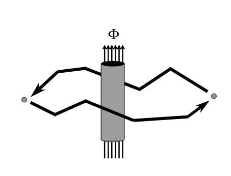
Figure 16: A topological interaction. The Aharonov-Bohm phase acquired by an electron that encircles a flux tube remains unchanged if the electron’s path is slightly deformed.

It is useful to reexpress this reasoning in the language of superselection rules. A superselection rule, as I am using the term here, arises (in a field theory or spin system defined in an infinite spatial volume) if Hilbert space decomposes into mutually orthogonal sectors, where each sector is preserved by any local operation. Perhaps the most familiar example is the charge superselection rule in quantum electrodynamics. An electric charge has an infinite range electric field. Therefore no local action can create or destroy a charge, for to destroy a charge we must also destroy the electric field lines extending to infinity, and no local procedure can accomplish this task.

The Aharonov-Bohm interaction is also an infinite range effect; the electron acquires an Aharonov-Bohm phase upon circling the solenoid no matter what its distance from the solenoid. So we may infer that no local operation can destroy a charge that participates in Aharonov-Bohm phenomena. If we consider two objects carrying such charges, widely separated and well isolated from other charged objects, then any process that changes the charge on either object would have to act coherently in the whole region containing the two charges. Thus, the charges are quite robust in the presence of localized disturbances; we can strike the particle with a hammer or otherwise abuse it without modifying the charges that it carries.

Following Kitaev,[25] we may envision a topological quantum computer, a device in which quantum information is encoded in the quantum numbers carried by quasiparticles that reside on a two–dimensional surface and have long-range Aharonov-Bohm interactions with one another. At zero temperature, an accidental exchange of quantum numbers between quasiparticles (an error) arises only due to quantum tunneling phenomena involving the virtual exchange of charged objects. The amplitude for such processes is of the order of $e^{-mL}$, where $m$ is the mass of the lightest charged object (in natural units), and $L$ is the distance between the two quasiparticles. If the quasiparticles are kept far apart, the probability of an error afflicting the encoded information will be extremely low. At finite temperature $T$, there is an additional source of error, because an uncontrolled plasma of charged particles will inevitably be present, with a density proportional to the Boltzman factor $e^{-\Delta/T}$, where $\Delta$ is the mass gap (not necessarily equal to the “curvature mass” $m$). Sometimes one of the plasma particles will slip unnoticed between two of our data-carrying particles, resulting in an exchange of charge and hence an error. To achieve an acceptably low error rate, then, we would need to keep the temperature well below the gap $\Delta$ (or else we would have to monitor the thermal plasma very faithfully).

7.2 The Fractional Quantum Hall Effect and Beyond

If our device is to be capable of performing interesting computations, the Aharonov-Bohm phenomena that it employs must be nonabelian. Only then will we be able to build up complex unitary transformations by performing many particle exchanges in succession. Such nonabelian Aharonov-Bohm effects can arise in systems with nonabelian gauge fields. Nature has been kind enough to provide us with some fundamental nonabelian gauge fields, but unfortunately not very many, and none of these seem to be suited for practical quantum computation. To realize Kitaev’s vision, then, we must hope that nonabelian Aharonov-Bohm effects can arise as complex collective phenomena in (two-dimensional electron or spin) systems that have only short-range fundamental interactions.

In fact, one of the most remarkable discoveries of recent decades has been that infinite range Aharonov-Bohm phenomena can arise in such systems, as revealed by the observation of the fractional quantum Hall effect. The electrons in quantum Hall systems are so highly frustrated that the ground state is an extremely entangled state with strong quantum correlations extending out over large distances. Hence, when one quasiparticle is transported around another, even when the quasiparticles are widely separated, the many electron wave function acquires a nontrivial Berry phase (such as $e^{2\pi i/3}$). This Berry phase is indistinguishable in all its observable effects from an Aharonov-Bohm phase arising from a fundamental gauge field, and its experimental consequences are spectacular.[55]

The Berry phases observed in quantum Hall systems are abelian (although there are some strong indications that nonabelian Berry phases can occur under the right conditions[56, 57]), and so are not very interesting from the viewpoint of quantum computation. But Kitaev[25] has described a family of simple spin systems with local interactions in which the existence of quasiparticles with nonabelian Berry phases can be demonstrated. (The Hamiltonian of the system so frustrates the spins that the ground state is a highly entangled state with infinite range quantum correlations.) These models are sufficiently simple (although unfortunately they require four-body interactions), that one can imagine a designer material that can be reasonably well-described by one of Kitaev’s models. The crucial topological properties of the model are relatively insensitive to the precise microscopic details, so the task of the fabricator who “trims” the material may not be overly demanding. If furthermore it were possible to control the transport of individual quasiparticles (perhaps with a suitable magnetic tweezers), then the system could be operated as a fault-tolerant quantum computer.

Figure 17: A Kitaev spin model. Spins reside on the lattice links. The four spins that meet at a site or share a plaquette are coupled.

To construct his models, Kitaev considers a square lattice, with spins residing on each lattice link. The Hamiltonian is expressed as a sum of mutually commuting four-body operators, one for each site and one for each plaquette of the lattice. (See Fig. 17.) Because the terms are mutually commuting, it is simple to diagonalize the Hamiltonian by diagonalizing each term separately. The operators on sites resemble local gauge symmetries (acting independently at each site), and a state that minimizes these terms is invariant under the local symmetry, like the physical states that obey Gauss’s law in a gauge theory. The operators on plaquettes are like “magnetic flux” operators in a gauge theory, and these terms are minimized when the magnetic flux vanishes everywhere. The excitation spectrum includes states in which Gauss’s law is violated at isolated sites — these points are “electrically charged” quasiparticles — and states in which the magnetic flux is nonvanishing at isolated plaquettes — these are magnetic fluxon quasiparticles. The quantum entanglement of the ground state is such that a nontrivial Berry phase is associated with the transport of a charge around a flux — this phase is identical to the Aharonov-Bohm phase in the analog gauge theory.

These Aharonov-Bohm phenomena are stable even as we deform the Hamiltonian of the theory. Indeed, if the deformation is sufficiently small, we can study its effects using perturbation theory. But as long as the perturbations are local in space, topological effects are robust, since perturbation theory is just a sum over localized influences. Whatever destroys the long-range topological interactions must be nonperturbative in the deformation of the theory.

Two types of nonperturbative effects can be anticipated.[58] The ground state of the theory might become a “flux condensate” with an indefinite number of magnetic excitations. In this event, there would be a long-range attractive interaction between charged particles and their antiparticles. It would be impossible to separate charges, and there would be no long-range effects. In a gauge theory, this phenomenon would be called electric confinement. Alternatively, a condensate of electric quasiparticles might appear in the ground state. Then the magnetic excitations would be confined, and again the long-range Aharonov-Bohm effects would be destroyed. In a gauge theory, we would call this the Higgs phenomenon (or magnetic confinement).

Thus, as we deform Kitaev’s Hamiltonian, we can anticipate that a phase boundary will eventually be encountered, beyond which either electric confinement or the Higgs phenomenon will occur. The size of the region enclosed by this boundary will determine how precisely a material will need to be fabricated in order to behave as Kitaev specifies. A particularly urgent question for the material designer is whether cleverly chosen two-body interactions might so frustrate a spin system as to produce a highly entangled ground state and nonabelian Aharonov-Bohm interactions among the quasiparticle excitations.

The fractional quantum Hall effect, and Kitaev’s models, speak a memorable lesson. We find gauge phenomena emerging as collective effects in systems with only short range interactions. It is intriguing to speculate that the gauge symmetries known in Nature could have a similar origin.

7.3 Topological Interactions

As we have noted, in Kitaev’s spin models, there are two types of charges that can be carried by localized quasiparticles, which we may call “electric” and “magnetic” charges. In the simplest type of model, the “magnetic flux” carried by a particle can be labeled by an element of a finite group $G$, and “electric charges” are labeled by irreducible representations of $G$. If a charged particle in the irreducible representation $D^{(\nu)}$, whose quantum numbers are encoded in an internal wavefunction $|\psi^{(\nu)}\rangle$, is carried around a flux labeled by group element $u\in G$, then the wavefunction is modified according to

$$|\psi^{(\nu)}\rangle\to D^{(\nu)}(u)|\psi^{(\nu)}\rangle\ .$$ (38)

Exploiting this interaction, we can measure a magnetic flux by scattering a suitable charged particle off of the flux.[59] For example, we could construct a Mach-Zender flux interferometer as shown in Fig. 18 that is sensitive to the relative phase acquired by the charged particle paths that pass to the left or right of the flux. If we balance the interferometer properly, we can distinguish between, say, two flux values $u_{1},u_{2}\in G$; a $u_{1}$ flux will be detected emerging from one arm of the interferometer, and a $u_{2}$ flux from the other arm. Of course, the interferometer we build will not be flawless, but the flux measurement can nevertheless be fault-tolerant — if we have many charged projectiles and perform the measurement repeatedly, we can determine the flux with very high statistical confidence.

Figure 18: A Mach-Zender interferometer for flux measurement, shown schematically. The flux to be measured is inserted inside. The test charge emerges from one arm if the flux has value $u_{1}$, the other arm if the flux has value $u_{2}$.

If the two fluxes $u_{1}$ and $u_{2}$ belong to the same conjugacy class in $G$, then there is a symmetry relating the two fluxons, so that all local physics is indifferent to the value of the flux (see below). Therefore, a coherent superposition of fluxes

$$a|u_{1}\rangle+b|u_{2}\rangle$$ (39)

will not readily decohere due to localized interactions with the environment. But the flux interferometer (operated repeatedly) will project the fluxon onto either of the flux eigenstates $|u_{1}\rangle$ (with probability $|a|^{2}$) or $|u_{2}\rangle$ (with probability $|b|^{2}$).

Figure 19: The flux exchange interaction. The flux labeled $u_{1}$ is carried from its original position (shaded) to its new position (unshaded), and then remeasured. The charged particle path shown that encircles the original position of the flux is topologically equivalent to a path that encircles the new position; hence the value of the flux changes from $u_{1}$ to $u_{1}^{\prime}=u_{2}^{-1}u_{1}u_{2}$.

Now imagine that two fluxons have been carefully calibrated, so that one is known to carry the flux $u_{1}$ and the other the flux $u_{2}$. And suppose that the two vortices are carefully “exchanged” by carrying the first around the second as shown in Fig. 19, and that we subsequently remeasure the fluxes. Carrying a charged particle around the fluxon on the right, after the exchange, is topologically equivalent to carrying the charged particle around first the right fluxon, then the left fluxon, and finally the right fluxon in the opposite direction, before the exchange. We infer that the exchange modifies the quantum numbers of the fluxons according to

$$|u_{1}\rangle|u_{2}\rangle\to|u_{2}\rangle|u_{2}^{-1}u_{1}u_{2}\rangle\ ,$$ (40)

a nontrivial interaction if the two fluxes fail to commute.[60] Thus, noncommuting fluxes have interesting Aharonov-Bohm interactions of their own, even in the absence of any electric charges. Because carrying one flux around another can conjugate the value of the flux, two fluxons carrying conjugate fluxes must be regarded as indistinguishable particles.[61] An exchange of two such objects can modify their internal quantum numbers; we will refer to them as nonabelions,[62] indistinguishable particles in two dimensions that obey an exotic nonabelian variant of quantum statistics.

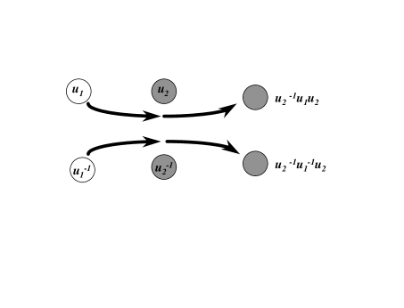
Figure 20: The “pull-through” interaction. One flux pair is pulled through another. The outside flux is unmodified, but the inside flux is conjugated by the outside flux.

We will use the exchange interaction Eq. (40) as a fundamental logical operation in our Aharonov-Bohm quantum computer. However, it will actually be convenient to encode qubits in pairs of fluxons, where the total flux of the pair is trivial.[25] That is, we will consider fluxon-antifluxon pairs of the form $|u,u^{-1}\rangle$, but where the flux and antiflux are kept far enough apart from one another that an inadvertent exchange of quantum numbers between them is unlikely. To perform logic, we may pull one pair through another as shown in Fig. 20. Since the total flux that passes through the middle of the outside pair is trivial, this pair is not modified, but the inside fluxes are conjugated by the outside flux:

$$|u_{1},u_{1}^{-1}\rangle|u_{2},u_{2}^{-1}\rangle\to|u_{2},u_{2}^{-1}\rangle|u_{2}^{-1}u_{1}u_{2},u_{2}^{-1}u_{1}^{-1}u_{2}\rangle\ ;$$ (41)

an operation that is evidently isomorphic to the effect of the exchange of single fluxes described by Eq. (40). Using pairs instead of single fluxons has two advantages. First, since each pair has trivial total flux, the pairs do not interact unless one is pulled through another; therefore, we can easily shunt pairs around the device without inducing any unwanted interactions with distant pairs. Second, and more important, pairs can carry charges even if each member of the pair carries no charge.[63, 64] The charge of a pair can be measured, and this charge-measurement operation will be a crucial ingredient in the construction of a universal set of quantum gates. The operation Eq. (41) can be regarded as a classical logic gate; it takes flux eigenstates to flux eigenstates. To perform interesting quantum computations, we will need to be able to prepare coherent superpositions of flux eigenstates. This is what we can accomplish by measuring the charge of a pair.

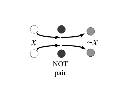
Figure 21: The NOT gate. Pulling a computational flux pair through a NOT pair flips the value of the encoded bit.

Figure 22: A Mach-Zender interferometer for charge measurement, shown schematically. The flux pair whose charge is to be measured is inserted inside. If the test NOT flux emerges from one arm, the $|+\rangle$ charge state has been prepared; if it emerges from the other arm, $|-\rangle$ has been prepared.

Suppose that $u_{0}$ and $u_{1}\in G$ are related by $u_{1}=v^{-1}u_{0}v$ for some $v\in G$. Then if we think of the flux eigenstates $|u_{0},u_{0}^{-1}\rangle$ and $|u_{1},u_{1}^{-1}\rangle$ as computational basis states, the effect of pulling either pair through a $|v,v^{-1}\rangle$ pair can be interpreted as a NOT or $X$ gate:

$$|u_{0},u_{0}^{-1}\rangle\leftrightarrow|u_{1},u_{1}^{-1}\rangle$$ (42)

(see Fig. 21). But suppose we wish to prepare one of the states

$$|\pm\rangle={1\over\sqrt{2}}\left(|u_{0},u_{0}^{-1}\rangle\pm|u_{1},u_{1}^{-1}\rangle\right)\ .$$ (43)

We can project a coherent superposition of $|u_{0},u_{0}^{-1}\rangle$ and $|u_{1},u_{1}^{-1}\rangle$ onto the $\{|\pm\rangle\}$ basis by scattering a $|v\rangle$ fluxon off the pair, or in other words by operating a charge interferometer, as in Fig. 22. When the $|v\rangle$ fluxon navigates around the pair, it acquires a trivial Aharonov-Bohm phase if the pair is in the state $|+\rangle$ and the nontrivial phase $-1$ if the pair is in the state $|-\rangle$. If the interferometer is properly balanced, then, the $|v\rangle$ projectile will be detected emerging from one arm of the interferometer if the pair is $|+\rangle$, and the other arm if the pair is $|-\rangle$. This is an example of charge measurement. Though the interferometer will not be perfect, charge measurement (like flux measurement) can be fault-tolerant, if we repeat the measurement enough times.

7.4 Universal Topological Computation

Working with fluxon pairs as computational basis states, we have seen how to perform the exchange (or “pull through”) operation Eq. (41), how to measure flux (using previously calibrated charges), and how to measure charge (using previously calibrated fluxes). We will also suppose that we are able to produce a large supply of vortex pairs. Local processes produce pairs that carry no charge or flux; a charge-zero pair with trivial flux has the form (up to normalization)

$$|{\rm charge~{}~{}zero}\rangle=\sum_{u}|u,u^{-1}\rangle\ ,$$ (44)

where the sum ranges over a complete conjugacy class of $G$. Because this state is left invariant when conjugated by any element of $G$, it has trivial Aharonov-Bohm interactions with any flux, and so carries no detectable charge. After producing such a pair, we can perform flux measurement to project out one of the flux eigenstate pairs $|u,u^{-1}\rangle$. Performing many such measurements on many pairs, we can assemble a large reservoir of calibrated flux pairs that can be withdrawn as needed during the course of a computation.

But is our quantum computer universal — can we closely approximate any desired unitary transformation? To address this issue, we recall the result mentioned in §4.2: Universal classical computation, together with the ability to perform the single-qubit gates $X$ and $Z$, and the ability to measure $X$, $Y$, and $Z$, suffice for universal quantum computation.[17] In fact, there are groups $G$ such that the operation Eq. (41) is sufficient for universal classical computation. We have found[65] that a Toffoli gate can be constructed from Eq. (41) if $G=A_{5}$, the group of even permutations on five objects. We may, for example, choose computational basis states with

$$u_{0}=(125)\ ,\quad u_{1}=(234)\ ;$$ (45)

that is, we choose our computational fluxes to be three-cycles with one object in common. Then a Toffoli gate can be constructed from a total of 16 elementary “pull-through” operations; six ancilla pairs are also used to catalyze this reaction. No Toffoli gate was found in any group smaller than $A_{5}$. Since $A_{5}$ is also the smallest of the finite nonsolvable groups, it is tempting to conjecture that nonsolvablility is a necessary condition for universal classical computation generated by conjugation.

We have already remarked that an $X$ gate can be realized by pulling a computational vortex pair through the pair with flux $v$ such that $u_{1}=v^{-1}u_{0}v$; here we choose $v=(14)(35)$. It turns out that the $Z$ gate can be constructed with six pull-through steps and four ancilla pairs. Measuring $Z$ is the same as measuring flux, and we have already seen that $X$ measurement can be achieved by measuring the charge of a pair, specifically, by using a $v$ projectile in a charge interferometer. It only remains to verify that we can measure $Y$. Though $Y$ measurement cannot be carried out exactly in this scheme, it turns out that a controlled-$Y$ gate can be constructed from 31 pull-through steps, and using 7 ancilla pairs. Appealing to another trick invented by Kitaev,[67] we can use the controlled-$Y$ gate repeatedly to carry out $Y$-measurement to any desired accuracy. Therefore, we have constructed a universal gate set using only the Aharonov-Bohm interactions of fluxes and charges; we have a fault-tolerant universal quantum computer.

Unfortunately, the spin model on which this construction is based is not so simple. Since the group $A_{5}$ has order 60, the Kitaev spin model that realizes this scenario has a 60-component spin residing at each lattice link (!) One hopes that a simpler implementation of universal Aharonov-Bohm computation will be found.

7.5 Is Nature Fault Tolerant?

The discovery of quantum error correction and fault tolerance has so altered our thinking about quantum information that it is appropriate to wonder about the potential implications for fundamental physics. And in fact, a fundamental issue pertaining to loss of quantum information has puzzled the physics community for over twenty years.

In 1975, Stephen Hawking[68] argued that quantum information is unavoidably lost when a black hole forms and then subsequently evaporates completely. The essence of the argument is very simple: because of the highly distorted causal structure of the black hole spacetime, the emitted radiation is actually on the same time slice as the collapsing body that disappeared behind the event horizon. If the quantum information that is initially encoded in the collapsing body is eventually to re-emerge encoded in the microstate of the emitted information, then that information must be in two places at once. In other words, the quantum information must be cloned, a known impossibility under the usual assumptions of quantum theory.[69, 70] Hawking concludes that not all physical processes can be governed by unitary time evolution; the laws of quantum theory need revision.

This argument is persuasive, but many physicists are very distrustful of the conclusion. Perhaps one reason for the skepticism is that it seems odd for Nature to tolerate just a little bit of information loss.[71] If processes involving black holes can destroy information, then one expects that information loss is unsuppressed at the Planck length scale $(G\hbar/c^{3})^{1/2}\sim 10^{-33}$ cm, a scale where virtual black holes continually arise as quantum fluctuations. It becomes hard to understand why quantum information can be so readily destroyed at the Planck scale, yet is so well preserved at the much longer distance scales that we have been able to explore experimentally — violations of quantum mechanics, after all, have never been observed.

Our newly acquired understanding of fault–tolerant quantum computation provides us with a fresh and potentially fruitful way to think about this problem. In Kitaev’s spin models, we might imagine that localized processes that destroy quantum information are quite common. Yet were we to follow the evolution of the system with coarser resolution, tracking only the information encoded in the charges of distantly separated quasiparticles, we would observe unitary evolution to remarkable accuracy; we would detect no glimmer of the turmoil beneath the surface.

Likewise, it is tempting to speculate that Nature has woven fault tolerance into her design, shielding the quantum noise at the Planck scale from our view. The discovery that quantum systems can be stabilized through suitable coding methods prompts us to ask the question: Is Nature fault tolerant? If so, then quantum mechanics may reign (to excellent accuracy) at intermediate length scales, but falter both at the Planck scale (where “errors” are common) and at macroscopic scales (where decoherence is rapid).

References

References

- [1] R. P. Feynman, Simulating physics with computers, Int. J. Theor. Phys. 21, 467 (1982).
- [2] D. Deutsch, Quantum theory, the Church-Turing principle and the universal quantum computer, Proc. Roy. Soc. Lond. A 400, 96 (1985).
- [3] P. Shor, Algorithms for quantum computation: discrete logarithms and factoring, in Proceedings of the 35th Annual Symposiumoon Fundamentals of Computer Science (Los Alamitos, CA, IEEE Press, 1994), pp. 124-134.
- [4] R. Landauer, Is quantum mechanics useful? Phil. Tran. R. Soc. Lond. 353, 367 (1995).
- [5] R. Landauer, The physical nature of information, Phys. Lett. A 217, 188 (1996).
- [6] R. Landauer, Is quantum mechanically coherent computation useful? In Proc. Drexel-4 Symposium on Quantum Nonintegrability-Quantum-Classical Correspondence, Philadelphia, PA, 8 September 1994, ed. D. H. Feng and B.-L. Hu (Boston, International Press, 1997).
- [7] W. G. Unruh, Maintaining coherence in quantum computers, Phys. Rev. A 51, 992 (1995).
- [8] S. Haroche and J. M. Raimond, Quantum computing: dream or nightmare? Phys. Today 49 (8), 51 (1996).
- [9] W. H. Zurek, Decoherence and the transition from quantum to classical, Phys. Today 44, 36 (1991).
- [10] P. Shor, Scheme for reducing decoherence in quantum memory, Phys. Rev. A 52, 2493 (1995).
- [11] A. M. Steane, Error correcting codes in quantum theory, Phys. Rev. Lett. 77, 793 (1996).
- [12] A. M. Steane, Multiple particle interference and quantum error correction, Proc. Roy. Soc. Lond. A 452, 2551 (1996).
- [13] J. von Neumann, Probabilistic logics and synthesis of reliable organisms from unreliable components, in Automata Studies, ed. C. E. Shannon and J. McCarthy (Princeton, Princeton University Press, 1956).
- [14] P. Gaćs, Reliable computation with cellular automata, J. Comp. Sys. Sci 32, 15 (1986).
- [15] P. Shor, Fault-tolerant quantum computation, in Proceedings of the Symposium on the Foundations of Computer Science (Los Alamitos, CA: IEEE Press, online preprint quant-ph/9605011, 1996).
- [16] A. M. Steane, Active stabilization, quantum computation and quantum state synthesis, Phys. Rev. Lett. 78, 2252 (1997).
- [17] D. Gottesman, A theory of fault-tolerant quantum computation (online preprint quant-ph/9702029, 1997).
- [18] E. Knill and R. Laflamme, Concatenated quantum codes (online preprint quant-ph/9608012, 1996).
- [19] E. Knill, R. Laflamme, and W, Zurek, Accuracy threshold for quantum computation, (online preprint quant-ph/9610011, 1996).
- [20] E. Knill, R. Laflamme, and W. Zurek, Resilient quantum computation: error models and thresholds (online preprint quant-ph/9702058, 1997).
- [21] D. Aharonov and M. Ben-Or, Fault tolerant quantum computation with constant error (online preprint quant-ph/9611025, 1996).
- [22] A. Yu. Kitaev, Quantum computing: algorithms and error correction, (preprint, in Russian, 1996).
- [23] J. Preskill, Reliable quantum computers (online preprint quant-ph/9705031, 1997).
- [24] C. Zalka, Threshold estimate for fault tolerant quantum computing (online preprint quant-ph/9612028, 1996).
- [25] A. Yu. Kitaev, Fault-tolerant quantum computation by anyons (online preprint quant-ph/9707021, 1997).
- [26] F. J. MacWilliams and N. J. A. Sloane, The Theory of Error-Correcting Codes, (New York, North-Holland Publishing Company, 1977).
- [27] E. Knill and R. Laflamme, A theory of quantum error-correcting codes, Phys. Rev. A 55, 900 (1997).
- [28] A. R. Calderbank and P. W. Shor, Good quantum error-correcting codes exist, Phys. Rev. A 54, 1098 (1996).
- [29] D. Gottesman, Class of quantum error-correcting codes saturating the quantum Hamming bound. Phys. Rev. A 54, 1862 (1996).
- [30] A. R. Calderbank, E. M. Rains, P. W. Shor, and N. J. A. Sloane, Quantum error correction and orthogonal geometry, Phys. Rev. Lett. 78, 405 (1997).
- [31] A. R. Calderbank, E. M. Rains, P. W. Shor, and N. J. A. Sloane, Quantum error correction via codes over GF(4) (online preprint quant-ph/9608006, 1996).
- [32] J. Evslin, S. Kakade, and J. Preskill, unpublished (1996).
- [33] D. DiVincenzo and P. Shor, Fault-tolerant error correction with efficient quantum codes. Phys. Rev. Lett. 77, 3260 (1996).
- [34] A. Yu. Kitaev, Quantum error correction with imperfect gates, (preprint, 1996).
- [35] D. Gottesman, Stabilizer codes and quantum error correction. Ph.D. thesis, California Institute of Technology (online preprint quant-ph/9705052, 1997).
- [36] C. Bennett, D. DiVincenzo, J. Smolin, and W. Wootters, Mixed state entanglement and quantum error correction, Phys. Rev. A 54, 3824 (1996).
- [37] R. Laflamme, C. Miquel, J. P. Paz, and W. Zurek, Perfect quantum error correction code, Phys. Rev. Lett. 77, 198 (1996).
- [38] D. Gottesman and J. Preskill, unpublished (1997).
- [39] D. Gottesman, J. Evslin, S. Kakade, and J. Preskill, unpublished (1996).
- [40] K. Obenland and A. M. Despain, Simulation of factoring on a quantum computer architecture, in Proceedings of the 4th Workshop on Physics and Computation, Boston, November 22-24, 1996, (Boston, New England Complex Systems Institute, 1996).
- [41] K. Obenland, and A. M. Despain, Impact of errors on a quantum computer architecture (online preprint http://www.isi.eu/acal/quantum/ quantum_op_errors.ps, 1996).
- [42] C. Miquel, J. P. Paz, and W. H. Zurek, Quantum computation with phase drift errors (online preprint quant-ph/9704003, 1997).
- [43] J. I. Cirac and P. Zoller, Quantum computations with cold trapped ions, Phys. Rev. Lett. 74, 4091 (1995).
- [44] M. B. Plenio and P. L. Knight, Decoherence limits to quantum computation using trapped ions, Proc. Roy. Soc. Lond. A 453, 2017 (1997).
- [45] M. Grassl, Th. Beth, and T. Pellizzari, Codes for the quantum erasure channel, Phys. Rev. A 56, 33 (1997).
- [46] A. K. Lenstra, J. Cowie, M. Elkenbracht-Huizing, W. Furmanski, P. L. Montgomery, D. Weber, J. Zayer, RSA factoring-by-web: the world-wide status (online document http: //www.npac.syr.edu/factoring/ status.html, 1996).
- [47] D. Beckman, A. Chari, S. Devabhaktuni, and J. Preskill, Efficient networks for quantum factoring, Phys. Rev. A 54, 1034 (1996).
- [48] A. M. Steane, Space, time, parallelism and noise requirements for reliable quantum computing (online preprint quant-ph/9708021, 1997).
- [49] C. Monroe, D. M. Meekhof, B. E. King, W. M. Itano, and D. J. Wineland, Demonstration of a fundamental quantum logic gate, Phys. Rev. Lett. 75, 4714 (1995).
- [50] Q. A. Turchette, C. J. Hood, W. Lange, H. Mabuchi, and H. J. Kimble, Measurement of conditional phase shifts for quantum logic. Phys. Rev. Lett. 75, 4710 (1995).
- [51] D. G. Cory, A. F. Fahmy, and T. F. Havel, Nuclear magnetic resonance spectroscopy: an experimentally accessible paradigm for quantum computing. In Proceedings of the 4th Workshop on Physics and Computation (Boston, New England Complex Systems Institute, 1996).
- [52] N. Gershenfeld and I. Chuang, Bulk spin resonance quantum computation. Science 275, 350 (1997).
- [53] J. Preskill, Quantum computing: pro and con (online preprint quant-ph/9705032, 1997).
- [54] S. Lloyd, Universal quantum simulators, Science 273, 1073 (1996).
- [55] R. Prange and S. Girvin, eds., The Quantum Hall Effect (New York, Springer-Verlag, 1987).
- [56] N. Read and E. Rezayi, Quasiholes and fermionic zero modes of paired fraction quantum Hall states: the mechanism for nonabelian statistics (online preprint cond-mat/9609079, 1996).
- [57] C. Nayak and F. Wilczek, quasihole states realize -dimensional spinor braiding statistics in paired quantum Hall states (online preprint cond-mat/9605145, 1996).
- [58] G, ’t Hooft, On the phase transition toward permanent quark confinement, Nucl. Phys. B 138, 1 (1978).
- [59] M. Alford, S. Coleman, and J. March-Russell, Disentangling nonabelian discrete quantum hair, Nucl. Phys. B 351, 735 (1991).
- [60] F. A. Bais, Flux metamorphosis, Nucl. Phys. B 170, 32 (1980).
- [61] H.-K. Lo and J. Preskill, Nonabelian vortices and nonabelian statistics, Phys. Rev. D 48, 4821 (1993)
- [62] G. Moore and N. Read, Nonabelions in the fractional quantum Hall effect, Nucl. Phys. B 360, 362 (1991).
- [63] M. G. Alford, K. Benson, S. Coleman, J. March-Russell, and F. Wilczek, Interactions and excitations of nonabelian vortices, Phys. Rev. Lett. 64, 1632 (1990).
- [64] J. Preskill and L. M. Krauss, Local discrete symmetry and quantum mechanical hair, Nucl. Phys. B 341, 50 (1990).
- [65] W. Ogburn and J. Preskill, unpublished (1997).
- [66] D. A. Barrington, Bounded width polynomial size branching programs recognoze exactly those languages in , J. Comp. Sys. Sci. 38, 150-164 (1989).
- [67] A. Yu. Kitaev, Quantum measurements and the abelian stabilizer problem (online preprint quant-ph/9511026, 1995).
- [68] S. W. Hawking, Breakdown of predictability in gravitational collapse, Phys. Rev. D 14, 2460 (1976).
- [69] D. Dieks, Communication by electron-paramagnetic-resonance devices. Phys. Lett. A 92, 271 (1982).
- [70] W. K. Wootters, and W. H. Zurek, A single quantum cannot be cloned, Nature 299, 802 (1982).
- [71] T. Banks, M. E. Peskin, and L. Susskind, Difficulties for the evolution of pure states into mixed states, Nucl. Phys. B 244, 125 (1984).