Direct and indirect strategies for phase measurement

Abstract

Recently, Torgerson and Mandel [Phys. Rev. Lett. 76, 3939 (1996)] have reported a disagreement between two schemes for measuring the phase difference of a pair of optical fields. We analyze these schemes and derive their associated phase-difference probability distributions, including both their strong and weak field limits. Our calculation confirms the main point of Torgerson and Mandel of the non-uniqueness of an operational definition of the phase distribution. We further discuss the role of postselection of data and argue that it cannot meaningfully improve the sensitivity.

I Introduction

Lack of a canonical pair for the number and phase operators, $\hat{n}$ and $\hat{\varphi}$, has led to much debate in quantum mechanics for many years now [1]. A more recent approach to the phase question involves concentrating more on what the experimentalist actually does: If his goal is a precision measurement then he can perform “any” measurement followed by data analysis to extract a classical parameter [2], for instance phase shift in an interferometer. Alternatively, he may mentally lump together the measurement and data analysis to construct an operational phase operator for his specific setup. This latter approach has been championed by Mandel and his coworkers [3, 4, 5, 6]. The explicit construction and investigation of the properties of such phase observables can give us insight into the nature of quantum states.

Recently, Torgerson and Mandel [7] have compared two schemes for measuring the phase-difference between a pair of optical fields. They found that a direct scheme, where a signal is beat against a second one, and an indirect scheme, where the two signals are beat against a common local oscillator, yield different probability distributions for the measured phase-difference. In particular, they found that the schemes gave radically different distributions for very weak signals. Torgerson and Mandel take the conflicting results as evidence of the non-uniqueness of quantum phase. In their analyses ambiguous data is discarded. This postselection procedure has generated some discussion in the literature [8, 9]. We analyze these two schemes in the absence and presence of this postselection and discuss its interpretation. We study limits for both strong and weak signals in these schemes and give closed form expressions for the phase-difference probability distributions.

II The NFM method

In the present section we review the operational definition of quantum phase based on the eight-port homodyne detector as well as its photon count statistics.

A NFM phase operators

The idea of Noh, Fougères and Mandel of operationally defined phase operators is guided by a classical analysis [10] of the eight-port homodyne interferometer [11] shown in Fig. 1. Replacing the classical light intensities at the four detectors $D_{i},(i=3,4,5,6)$ by number operators $\hat{n}_{i}=\hat{a}^{\dagger}_{i}\hat{a}_{i}$, NFM propose [3, 4, 5, 6, 10] the phase operators

$$\hat{C}_{M} \equiv \frac{\hat{n}_{4}-\hat{n}_{3}}{\sqrt{(\hat{n}_{4}-\hat{n}_{3})^{2}+(\hat{n}_{6}-\hat{n}_{5})^{2}}}\equiv\frac{\hat{n}_{43}}{\sqrt{\hat{n}_{43}^{2}+\hat{n}_{65}^{2}}}$$ (1)

and

$$\hat{S}_{M} \equiv \frac{\hat{n}_{6}-\hat{n}_{5}}{\sqrt{(\hat{n}_{4}-\hat{n}_{3})^{2}+(\hat{n}_{6}-\hat{n}_{5})^{2}}}\equiv\frac{\hat{n}_{65}}{\sqrt{\hat{n}_{43}^{2}+\hat{n}_{65}^{2}}}.$$ (2)

In the classical limit the operators $\hat{C}_{M}$ and $\hat{S}_{M}$ become [10] the cosine and sine of the phase difference between two classical electromagnetic fields in the modes 1 and 2. Hence we can consider these operators to be the extension of this classical description of phase into the quantum domain.

How can we calculate expectation values of a function $f$ of these operators $\hat{C}_{M}$ and $\hat{S}_{M}$? According to the NFM-prescription this expectation value reads

$$\langle f(\hat{C}_{M},\hat{S}_{M})\rangle\equiv{\cal N}\sum_{n_{43},n_{65}\neq 0}f\left(\frac{n_{43}}{\sqrt{n_{43}^{2}+n_{65}^{2}}},\frac{n_{65}}{\sqrt{n_{43}^{2}+n_{65}^{2}}}\right)W(n_{43},n_{65}),$$ (3)

where $W(n_{43},n_{65})$ denotes the joint count probability for the differences $n_{43}\equiv n_{4}-n_{3}$ and $n_{65}\equiv n_{6}-n_{5}$ at the four detectors. The sum in above equation is performed over all $n_{43}$ and $n_{65}$, except $n_{43}=n_{65}=0$. In order to avoid the problems associated with the definitions (1) and (2) for $n_{43}=n_{65}=0$, NFM disregard such measurements and renormalize the joint count probability via ${\cal N}=[1-W(0,0)]^{-1}$. The theoretical results obtained by NFM using this formalism are in very nice agreement [3, 4, 5, 6] with their experiments.

Equation (3) shows that the central quantity in the NFM approach is the joint count probability [12, 13, 14]

$$W(n_{43},n_{65})=\mathop{{\sum}^{\prime}}_{n_{3},n_{4},n_{5},n_{6}}\langle n_{3},n_{4},n_{5},n_{6}|\hat{\rho}_{\rm out}|n_{3},n_{4},n_{5},n_{6}\rangle,$$ (4)

where $\hat{\rho}_{\rm out}$ is the density operator of the four input modes of the interferometer after transformation through the beam splitters and the $\lambda/4$ plate. The ket $|n_{3},n_{4},n_{5},n_{6}\rangle$ denotes the product number state corresponding to the four output modes and the summation $\sum^{\prime}$ is performed for fixed differences $n_{43}$ and $n_{65}$.

B Eight-port homodyne count statistics

We now consider the case in which the input density matrix is expressed in terms of coherent states, that is

$$\hat{\rho}_{\rm in}=\int d^{2}\beta_{1}d^{2}\beta_{2}P(\beta_{1},\beta_{2})|\beta_{1}\rangle_{1\;1}\langle\beta_{1}|\otimes|0\rangle_{10\;10}\langle 0|\otimes|\beta_{2}\rangle_{2\;2}\langle\beta_{2}|\otimes|0\rangle_{20\;20}\langle 0|,$$ (5)

where $P(\beta_{1},\beta_{2})$ is a two-mode Glauber-Sudarshan distribution for the fields entering ports 1 and 2. The output density operator just before photodetection reads

$$\hat{\rho}_{\rm out} = \int d^{2}\beta_{1}d^{2}\beta_{2}P(\beta_{1},\beta_{2})\left|{\textstyle{\frac{1}{2}}}(\beta_{1}-\beta_{2}e^{i\theta})\right\rangle_{3\;3}\left\langle{\textstyle{\frac{1}{2}}}(\beta_{1}-\beta_{2}e^{i\theta})\right|$$ (9)

$$\qquad{}\otimes\left|{\textstyle{\frac{1}{2}}}(\beta_{1}+\beta_{2}e^{i\theta})\right\rangle_{4\;4}\left\langle{\textstyle{\frac{1}{2}}}(\beta_{1}+\beta_{2}e^{i\theta})\right|$$

$${}\qquad\otimes\left|{\textstyle{\frac{1}{2}}}(-i\beta_{1}+\beta_{2}e^{i\theta})\right\rangle_{5\>5}\left\langle{\textstyle{\frac{1}{2}}}(-i\beta_{1}+\beta_{2}e^{i\theta})\right|$$

$${}\qquad\otimes\left|{\textstyle{\frac{1}{2}}}(-i\beta_{1}-\beta_{2}e^{i\theta})\right\rangle_{6\;6}\left\langle{\textstyle{\frac{1}{2}}}(-i\beta_{1}-\beta_{2}e^{i\theta})\right|,$$

where the phase shift $\theta$ was introduced into the field entering port 2 for reasons which will become clear in the next section.

We calculate the joint count probability for the differences $n_{43}$ and $n_{65}$ in the photocount distribution, for a given phase shift $\theta$, by substituting Eq. (9) into Eq. (4), and obtain

$$W(n_{43},n_{65}|e^{i\theta})=\int d^{2}\beta_{1}d^{2}\beta_{2}P(\beta_{1},\beta_{2})K_{43}K_{65},$$ (10)

where the kernels $K_{43}$ and $K_{65}$ are given by

$$K_{43} = \mathop{{\sum}^{\prime}}_{n_{3},n_{4}}\left|\langle n_{3}|{\textstyle{\frac{1}{2}}}(\beta_{1}-\beta_{2}e^{i\theta})\rangle\right|^{2}\left|\langle n_{4}|{\textstyle{\frac{1}{2}}}(\beta_{1}+\beta_{2}e^{i\theta})\rangle\right|^{2}$$ (11)

and

$$K_{65} = \mathop{{\sum}^{\prime}}_{n_{5},n_{6}}\left|\langle n_{5}|{\textstyle{\frac{1}{2}}}(-i\beta_{1}+\beta_{2}e^{i\theta})\rangle\right|^{2}\left|\langle n_{6}|{\textstyle{\frac{1}{2}}}(-i\beta_{1}-\beta_{2}e^{i\theta})\rangle\right|^{2}.$$ (12)

These sums have been previously computed [12, 15, 16] and we find

$$K_{43} = e^{-\frac{1}{2}(|\beta_{1}|^{2}+|\beta_{2}|^{2})}\left|\frac{\beta_{1}+\beta_{2}e^{i\theta}}{\beta_{1}-\beta_{2}e^{i\theta}}\right|^{n_{43}}I_{|n_{43}|}\left({\textstyle{\frac{1}{2}}}|\beta_{1}^{2}-\beta_{2}^{2}e^{2i\theta}|\right),$$ (13)

and

$$K_{65} = e^{-\frac{1}{2}(|\beta_{1}|^{2}+|\beta_{2}|^{2})}\left|\frac{i\beta_{1}+\beta_{2}e^{i\theta}}{i\beta_{1}-\beta_{2}e^{i\theta}}\right|^{n_{65}}I_{|n_{65}|}\left({\textstyle{\frac{1}{2}}}|\beta_{1}^{2}+\beta_{2}^{2}e^{2i\theta}|\right),$$ (14)

where $I_{\nu}(z)$ denotes the modified Bessel function of order $\nu$.

C Phase distributions from photon counts

An eight-port homodyne detector as shown in Fig. 1 measures the photon number differences $n_{43}$ and $n_{65}$ at the output. What we obtain are the probabilities, $W(n_{43},n_{65})$, as defined in Eq. (4), and we would like to use them to construct a phase distribution following the prescription given by NFM and summarized in Eqs. (1) and (2). This can be done by representing the pairs $(n_{43},n_{65})$ as points in a two-dimensional space where $n_{43}$ is the $x$ coordinate and $n_{65}$ is the $y$ coordinate. Eqs. (1) and (2) imply that a difference phase of $\varphi$ corresponds to a ray in this space which starts at the origin and makes an angle $\varphi$ with the positive $x$-axis. The probability assigned to $\varphi$ is just the sum of the probabilities of the points, $(n_{43},n_{65})$, which the ray passes through.

There are two problems with this prescription. The first is that the distribution will not be smooth; it will consist of a number of spikes. Certain rays will intersect no $(n_{43},n_{65})$ points yielding a value of zero for the probability of the corresponding angle, whereas a nearby ray will hit such a point which can lead to a nonzero probability for its angle. What is needed is a way to smooth the distribution and this has been provided by NFM, and we shall discuss it shortly. The second problem has to do with the contribution of the origin, $n_{43}=0$ and $n_{65}=0$, to the phase distribution. A glance at Eqs. (1) and (2) show that the sine and cosine are not defined at this point which implies that the angle is not defined either. One now has to decide what to do with the probability corresponding to this point when constructing the phase distribution. NFM throw out the data corresponding to this point and renormalize the remaining probabilities, $W(n_{43},n_{65})$ for $n_{43},n_{65}\neq 0$, accordingly. Another possibility is to associate $W(0,0)$ with a uniform distribution of the angle. The philosophy behind this approach is that because we have no information about how to assign $W(0,0)$ to any angle, we apportion it equally among all angles.

We follow the prescription in Sec. II A to obtain the two possible phase difference distributions

$${\cal P}_{0}(\varphi) = \langle\delta(\varphi-\hat{\varphi}_{M})\rangle=\left\langle\delta\left[\varphi-\arctan\left(\frac{\hat{S}_{M}}{\hat{C}_{M}}\right)\right]\right\rangle$$ (15)

$$= \frac{1}{1-W(0,0)}\sum_{n_{43},n_{65}\neq 0}W(n_{43},n_{65})\delta\left(\varphi-\arctan\frac{n_{65}}{n_{43}}\right),$$ (16)

and

$${\cal P}_{1}(\varphi)=\frac{1}{2\pi}W(0,0)+\sum_{n_{43},n_{65}\neq 0}W(n_{43},n_{65})\delta\left(\varphi-\arctan\frac{n_{65}}{n_{43}}\right),$$ (17)

where ${\cal P}_{0}(\varphi)$ is the distribution in which the origin has been eliminated and ${\cal P}_{1}(\varphi)$ is the distribution in which it has been included. In the above expressions [Eqs. (16) and (17)] and in all that follow one should be careful to choose the right branch of the function $\arctan$ according to the signs of $n_{43}$ and $n_{65}$.

The averaging procedure which was developed by NFM to smooth the phase distribution, and which is also used by Torgerson and Mandel, works in the following way. A phase shift of $\theta$ is introduced into the field entering port 2 of the 8-port detector. This produces new probabilities for the photon number differences at the output which we shall denote by $W(n_{43},n_{65}|e^{i\theta})$. Going back to our two-dimensional space, because the phase shift maps a phase difference of $\varphi$ into one of $\varphi-\theta$, a ray which makes an angle of $\varphi-\theta$ with the $x$-axis is associated with a phase shift of $\varphi$. This gives us a difference-phase distribution for each value of the phase shift $\theta$.

$${\cal P}_{0}(\varphi|\theta)=\langle\delta[\varphi-(\hat{\varphi}_{M}-\theta)]\rangle={\cal N}_{0}\sum_{n_{43},n_{65}\neq 0}W(n_{43},n_{65}|e^{i\theta})\delta\left[\varphi-\left(\arctan\frac{n_{65}}{n_{43}}-\theta\right)\right],$$ (18)

and

$${\cal P}_{1}(\varphi|\theta)=\frac{1}{2\pi}W(0,0|e^{i\theta})+\sum_{n_{43},n_{65}\neq 0}W(n_{43},n_{65}|e^{i\theta})\delta\left[\varphi-\left(\arctan\frac{n_{65}}{n_{43}}-\theta\right)\right].$$ (19)

We then obtain a final phase distribution by averaging

$$\overline{\cal P}(\varphi)=\frac{1}{2\pi}\int_{0}^{2\pi}d\theta\,{\cal P}(\varphi|\theta)$$ (20)

over all of them. The $\theta$ integrations are trivially performed, giving us

$$\overline{{\cal P}_{0}}(\varphi)=\frac{{\cal N}_{0}}{2\pi}\sum_{n_{43},n_{65}\neq 0}W\left(n_{43},n_{65}|e^{i(\arctan n_{65}/n_{43}-\varphi)}\right),$$ (21)

and

$$\overline{{\cal P}_{1}}(\varphi)=\frac{1}{2\pi}\left\{\frac{1}{2\pi}\int_{0}^{2\pi}d\theta\,W(0,0|e^{i\theta})+\sum_{n_{43},n_{65}\neq 0}W\left(n_{43},n_{65}|e^{i(\arctan n_{65}/n_{43}-\varphi)}\right)\right\},$$ (22)

where, as before, $\overline{{\cal P}_{0}}(\varphi)$ does not include the point $n_{43}=n_{65}=0$ and $\overline{{\cal P}_{1}}(\varphi)$ does. Note that in calculating $\overline{{\cal P}_{0}}(\varphi)$ we have first averaged the unnormalized distributions and then normalized the result. The constant ${\cal N}_{0}$ in Eq. (18) is chosen so that $\int_{0}^{2\pi}d\varphi\overline{{\cal P}_{0}}(\varphi)=1$. This is the procedure adopted by NFM. However, one could just as well normalize the distribution for each value of $\theta$ and then average the result. This will not give the same result as the first procedure because the normalization constant for each value of $\theta$, $(1-W(0,0|e^{i\theta}))^{-1}$, depends on $\theta$. There is no obvious reason to prefer one procedure over the other, so we simply use the one which was chosen by NFM.

III Schemes

Using the eight-port homodyne interferometer described in Sec. II B, Torgerson and Mandel [7] measure the phase difference between two coherent optical fields by (a) beating the two fields against each other and (b) by beating them against a common local oscillator. Torgerson and Mandel refer to these as the direct and indirect measurements. In this section we briefly describe these schemes and derive analytical expressions for the corresponding phase distributions.

A Direct scheme

The direct measurement is made by beating the two input fields against each other in a single eight-port homodyne interferometer. The expression for the phase distribution is then simply Eq. (21) [or Eq. (22)]. In what follows, we evaluate this expression in the limits of strong and weak fields.

1 Strong field limit

When one of the fields, say field 2, is strong we can use the known result for the strong local oscillator limit [13], where field 2 plays the role of the local oscillator. In this case, the phase distribution (both ${\cal P}_{0}$ and ${\cal P}_{1}$) reduces to

$${\cal P}(\varphi) = \frac{1}{\pi}\int d^{2}\beta_{1}\int d^{2}\beta_{2}\int_{0}^{\infty}rdrP(\beta_{1},\beta_{2})$$ (24)

$${}\times\exp\Bigl{\{}-\bigl{[}r\cos\varphi-|\beta_{1}|\cos(\phi_{2}-\phi_{1})\bigr{]}^{2}-\bigl{[}r\sin\varphi-|\beta_{1}|\sin(\phi_{2}-\phi_{1})\bigr{]}^{2}\Bigr{\}},$$

where $\beta_{j}=|\beta_{j}|e^{i\phi_{j}}$, for $j=1,2$.

2 Weak fields limit

When both fields are weak, we use the relation

$\displaystyle I_{\nu}(z)\simeq\frac{1}{\nu!}\left(\frac{z}{2}\right)^{\nu}$

for the modified Bessel function, which allows us to write the kernels in Eq. (10) as

$$K_{43}\simeq\left\{\begin{array}[]{lr}\displaystyle{\frac{e^{-\frac{1}{2}(|\beta_{1}|^{2}+|\beta_{2}|^{2})}}{4^{n_{43}}n_{43}!}}\left|\beta_{1}+\beta_{2}e^{i\theta}\right|^{2n_{43}},&n_{43}>0,\\ e^{-\frac{1}{2}(|\beta_{1}|^{2}+|\beta_{2}|^{2})},&n_{43}=0,\\ \displaystyle{\frac{e^{-\frac{1}{2}(|\beta_{1}|^{2}+|\beta_{2}|^{2})}}{4^{|n_{43}|}|n_{43}|!}}\left|\beta_{1}-\beta_{2}e^{i\theta}\right|^{2|n_{43}|},&n_{43}<0,\end{array}\right.$$ (25)

$$K_{65}\simeq\left\{\begin{array}[]{lr}\displaystyle{\frac{e^{-\frac{1}{2}(|\beta_{1}|^{2}+|\beta_{2}|^{2})}}{4^{n_{65}}n_{65}!}}\left|i\beta_{1}+\beta_{2}e^{i\theta}\right|^{2n_{65}},&n_{65}>0,\\ e^{-\frac{1}{2}(|\beta_{1}|^{2}+|\beta_{2}|^{2})},&n_{65}=0,\\ \displaystyle{\frac{e^{-\frac{1}{2}(|\beta_{1}|^{2}+|\beta_{2}|^{2})}}{4^{|n_{65}|}|n_{65}|!}}\left|i\beta_{1}-\beta_{2}e^{i\theta}\right|^{2|n_{65}|},&n_{65}<0.\end{array}\right.$$ (26)

The remaining integral in Eq. (22) is now trivially performed yielding

$\displaystyle\frac{1}{2\pi}\int_{0}^{2\pi}d\theta\,W(0,0|e^{i\theta})=\int d^{2}\beta_{1}d^{2}\beta_{2}P(\beta_{1},\beta_{2})e^{-(|\beta_{1}|^{2}+|\beta_{2}|^{2})}.$

In this limit, the sums in Eqs. (21) and (22) have only contributions from those terms in the lowest order in the coherent state amplitudes $|\beta_{j}|$. Hence only terms with $n_{43}=-1,0,1$ and $n_{65}=-1,0,1$ contribute and we arrive finally at

$$\overline{{\cal P}_{0}}(\varphi)\simeq\frac{{\cal N}_{0}}{2\pi}\int d^{2}\beta_{1}d^{2}\beta_{2}P(\beta_{1},\beta_{2})[|\beta-1|^{2}+|\beta_{2}|^{2}+2|\beta_{1}||\beta_{2}|\cos(\varphi+\phi_{1}-\phi_{2})],$$ (27)

and

$$\overline{{\cal P}_{1}}(\varphi)\simeq\frac{1}{2\pi}\int d^{2}\beta_{1}d^{2}\beta_{2}P(\beta_{1},\beta_{2})[1+2|\beta_{1}||\beta_{2}|\cos(\varphi+\phi_{1}-\phi_{2})],$$ (28)

up to corrections which are quartic in $|\beta_{j}|$. Note that Eq. (27) reproduces exactly the result obtained by Torgerson and Mandel [7],

$$\overline{{\cal P}_{0}}(\varphi)\simeq\frac{1}{2\pi}\left(1+\frac{2\cos(\varphi+\phi_{1}-\phi_{2})}{|\beta_{1}|/|\beta_{2}|+|\beta_{2}|/|\beta_{1}|}\right),$$ (29)

for input fields in coherent states $|\beta_{1}\rangle$ and $|\beta_{2}\rangle$. In this case, the phase distribution $\overline{{\cal P}_{1}}(\varphi)$, which includes the point $n_{43}=n_{65}=0$, reduces to

$$\overline{{\cal P}_{1}}(\varphi)\simeq\frac{1}{2\pi}\Bigl{[}1+2|\beta_{1}||\beta_{2}|\cos(\varphi+\phi_{1}-\phi_{2})\Bigr{]}.$$ (30)

B Indirect scheme

The indirect measurement scheme consists of two eight-port homodyne detectors, each performing a measurement of the phase distribution for one of the fields relative to a common strong local oscillator, $\alpha$, as seen in Fig. 2. Making no assumptions about the incoming state we could define the relative-phase distribution as the convolution

$${\cal P}(\varphi)=\int_{0}^{2\pi}d\varphi_{1}{\cal P}(\varphi_{1},\varphi_{1}-\varphi),$$ (31)

of the joint phase distribution

$${\cal P}(\varphi_{1},\varphi_{2})\equiv\frac{1}{\pi}\int_{0}^{\infty}r_{1}dr_{1}\int_{0}^{\infty}r_{2}dr_{2}\langle r_{1}e^{i\varphi_{1}},r_{2}e^{i\varphi_{2}}|\hat{\rho}|r_{1}e^{i\varphi_{1}},r_{2}e^{i\varphi_{2}}\rangle$$ (32)

which is the radially integrated two-mode $Q$-function, in terms of the two-particle state $\hat{\rho}$. We note that this reduces to the expected joint phase distribution

$${\cal P}(\varphi_{1},\varphi_{2})={\cal P}_{1}(\varphi_{1}){\cal P}_{2}(\varphi_{2}).$$ (33)

when the input fields are in the product state $\hat{\rho}=\hat{\rho}_{1}\otimes\hat{\rho}_{2}$ and where the individual phase distributions ${\cal P}_{i}(\varphi_{i})$ have their obvious meaning.

Let us now restrict our attention to the case where the input fields 1 and 2 have such a factorable state, so the two-mode $P$-function can be written $P(\beta_{1},\beta_{2})=P(\beta_{1})P(\beta_{2})$. Each phase distribution now takes the form

$${\cal P}_{i}(\varphi_{i}) = \frac{1}{\pi}\int d^{2}\beta_{i}P(\beta_{i})\int_{0}^{\infty}r_{i}dr_{i}$$ (35)

$${}\times\exp\Bigl{\{}-\bigl{[}r_{i}\cos\varphi_{i}-|\beta_{i}|\cos(\phi_{0}-\phi_{i})\bigr{]}^{2}-\bigl{[}r_{i}\sin\varphi_{i}-|\beta_{i}|\sin(\phi_{0}-\phi_{i})\bigr{]}^{2}\Bigr{\}},$$

where $\phi_{0}$ is the phase of the local oscillator and the $P(\beta_{i}),i=1,2$ are Glauber-Sudarshan distributions for the fields 1 and 2. Evaluating the integral in Eq. (31) we obtain the expression

$${\cal P}(\varphi) = \frac{2}{\pi}\int d^{2}\beta_{1}P(\beta_{1})\int d^{2}\beta_{2}\ P(\beta_{2})e^{-|\beta_{1}|^{2}-|\beta_{2}|^{2}}$$ (37)

$${}\times\int_{0}^{\infty}r_{1}dr_{1}\int_{0}^{\infty}r_{2}dr_{2}\;e^{-r_{1}^{2}-r_{2}^{2}}I_{0}\bigl{(}2|r_{1}\beta_{1}+r_{2}\beta_{2}e^{-i\varphi}|\bigr{)}$$

for the phase distribution of the indirect measurement. Again we now consider the limiting cases of this exact expression.

1 Strong field limit

In the case when the input field 2 is strong but still much weaker than the local oscillator, Eq. (37) approaches the result Eq. (24) for the direct measurement very quickly. This behavior can be seen from Fig. 3, where we have plotted both expressions for fields 1 and 2 in coherent states and $|\beta_{2}/\beta_{1}|=4$. For higher values of $|\beta_{2}|$ the two curves coincide.

2 Weak fields limit

In the case when both fields are weak, the Bessel function in Eq. (37) can be written as

$\displaystyle I_{0}(|z|)\simeq 1+\frac{|z|^{2}}{4}$

and the integral is easily performed yielding

$${\cal P}(\varphi)\simeq\frac{1}{2\pi}\int d^{2}\beta_{1}d^{2}\beta_{2}P(\beta_{1},\beta_{2})\left[1+\frac{\pi}{2}|\beta_{1}||\beta_{2}|\cos(\varphi+\phi_{1}-\phi_{2})\right]$$ (38)

to lowest order for the phase distribution.

We conclude this section by noting that, in contrast to the direct measurement, in this indirect measurement the contribution from ambiguous data is always negligible due to the presence of the strong local oscillator.

IV States with identical phase distributions

An unusual feature of the direct phase measurement scheme of Torgerson and Mandel (TM) is that any pair of two-mode input states which differ in their vacuum component, $|0,0\rangle$, will have the same phase distribution [4, 5]. For states with large photon numbers this is of little importance, but for states with very small photon numbers it has interesting consequences.

Let us first briefly show that this is true. Let $p(n_{3},n_{4},n_{5},n_{6}|\theta)$ be the probability that $D_{3}$ detects $n_{3}$ photons, $D_{4}$ detects $n_{4}$ photons, etc. (see Fig. 1), given that the phase of the input in port 2 has been shifted by $\theta$. If the two-field input state is $|\psi_{\rm in}\rangle$ and $\hat{U}(\theta)$ describes the action of the entire apparatus, with the phase shifter in port 2 set to $\theta$, then

$$p(n_{3},n_{4},n_{5},n_{6}|\theta)=|\langle n_{3},n_{4},n_{5},n_{6}|\hat{U}(\theta)|\psi_{\rm in},0,0\rangle|^{2},$$ (39)

where the two zeros appended to $|\psi_{\rm in}\rangle$ indicate that the other two inputs are in the vacuum state. Let us express $|\psi_{\rm in}\rangle$ as

$$|\psi_{\rm in}\rangle=c_{0}|0,0\rangle+|\Phi\rangle,$$ (40)

where $\langle\Phi|0,0\rangle=0$ and $|c_{0}|^{2}+\|\Phi\|^{2}=1$. Because the beam splitters and the phase shifter conserve total photon number we have

$$p(0,0,0,0|\theta) = |c_{0}|^{2},$$ (41)

$$p(n_{3},n_{4},n_{5},n_{6}|\theta) = |\langle n_{3},n_{4},n_{5},n_{6}|\hat{U}(\theta)|\Phi,0,0\rangle|^{2},\quad\hbox{\rm if $n_{3}+n_{4}+n_{5}+n_{6}\neq 0$}.$$ (42)

Now consider the input state

$$|\psi^{\prime}_{\rm in}\rangle=\frac{1}{\|\Phi\|}|\Phi\rangle$$ (43)

and denote the output photon number probabilities as $p^{\prime}(n_{3},n_{4},n_{5},n_{6}|\theta)$. (We note that this vacuum-depleted state $|\psi^{\prime}_{\rm in}\rangle$ will be typically an entangled state when the original $|\psi_{\rm in}\rangle$ is a two-mode product state.) Eq. (42) implies that for $n_{3}+n_{4}+n_{5}+n_{6}>0$,

$$p^{\prime}(n_{3},n_{4},n_{5},n_{6}|\theta)=\frac{1}{\|\Phi\|^{2}}p(n_{3},n_{4},n_{5},n_{6}|\theta).$$ (44)

Because events corresponding to $n_{j}=0$, $j=1,\dots,4$ are discarded, the probabilities $p(n_{3},n_{4},n_{5},n_{6}|\theta)$ and $p^{\prime}(n_{3},n_{4},n_{5},n_{6}|\theta)$, for $n_{3}+n_{4}+n_{5}+n_{6}>0$, determine the TM phase distributions for $|\psi_{\rm in}\rangle$ and $|\psi^{\prime}_{\rm in}\rangle$, respectively, and they are the same up to an overall factor. When the TM phase distributions for the two states are computed and normalized this factor disappears. Therefore, $|\psi_{\rm in}\rangle$ and $|\psi^{\prime}_{\rm in}\rangle$ have the same TM phase distribution.

Let us see what this implies for the input state considered by Torgerson and Mandel, two weak coherent states. We have for $|\beta_{1}|,|\beta_{2}|\ll 1$

$$|\psi_{\rm in}\rangle=|\beta_{1}\rangle\otimes|\beta_{2}\rangle\simeq e^{-\frac{1}{2}(|\beta_{1}|^{2}+|\beta_{2}|^{2})}(|0,0\rangle+\beta_{1}|1,0\rangle+\beta_{2}|0,1\rangle).$$ (45)

A consequence of the result in the previous paragraph is that the state

$$|\psi^{\prime}_{\rm in}\rangle=\left(\frac{1}{|\beta_{1}|^{2}+|\beta_{2}|^{2}}\right)^{1/2}(\beta_{1}|1,0\rangle+\beta_{2}|0,1\rangle)$$ (46)

has the same TM phase distribution as $|\psi_{\rm in}\rangle$ which is given by Eq. (29), i.e.

$\displaystyle{\cal P}(\varphi)\simeq\frac{1}{2\pi}\left(1+\frac{2\cos(\varphi+\phi_{1}-\phi_{2})}{|\beta_{1}|/|\beta_{2}|+|\beta_{2}|/|\beta_{1}|}\right).$

This fact has been noted by NFM [4, 5]. Torgerson and Mandel pointed out that the agreement between the above phase distribution, which agreed with their measurements, and the London distribution for $|\psi_{\rm in}\rangle$ is poor. Suppose we instead compare Eq. (29) to the London distribution for the state $|\psi^{\prime}_{\rm in}\rangle$. We find that they are identical.

One interpretation of these results is the following. If ${\cal P}(\varphi)$ is taken to be the TM phase distribution of $|\psi_{\rm in}\rangle$ one has the rather puzzling result that as $|\beta_{1}|$ and $|\beta_{2}|$ go to zero, with $|\beta_{1}|/|\beta_{2}|$ fixed, the phase distribution does not change. One would expect that as $|\psi_{\rm in}\rangle$ becomes closer to the vacuum its phase distribution would become more uniform. On the other hand, if ${\cal P}(\varphi)$ is interpreted as the phase distribution for $|\psi^{\prime}_{\rm in}\rangle$ the puzzle disappears. If $|\beta_{1}|$ and $|\beta_{2}|$ go to zero, with $|\beta_{1}|/|\beta_{2}|$ fixed, the state $|\psi^{\prime}_{\rm in}\rangle$ does not change and, therefore, neither should its phase distribution. Furthermore, its operational phase distribution (obtained via the direct measurement procedure) agrees with its London phase distribution. Because it discards data, the measurement procedure of Torgerson and Mandel is insensitive to the vacuum component of input states, which, along with the previous two observations, suggests that what is being measured is the phase distribution of $|\psi^{\prime}_{\rm in}\rangle$ and not that of $|\psi_{\rm in}\rangle$. This observation is closely related to one by Hradil in his discussion of the original Noh, Fougères, and Mandel proposal [3, 4, 8].

Another objection which can be raised to the interpretation of Eq. (29) as a phase distribution for $|\psi_{\rm in}\rangle$ has to do with the connection between a phase distribution and the rotational properties of its corresponding state in phase space. A useful property for a phase distribution to have is providing information about how distinguishable a state is from a rotated version of itself. A phase distribution with this property will be able to tell us how useful a given state is for the measurement of phase shifts. In the case of two-mode states we would like the difference-phase distribution of a state $|\psi\rangle$ to give us information about $|\langle\psi|\hat{U}_{D}(\varphi_{0})|\psi\rangle|$, which is a measure of how distinguishable $|\psi\rangle$ is from its difference-phase rotated version, $\hat{U}_{D}(\varphi_{0})|\psi\rangle$. Here the operator $\hat{U}_{D}(\varphi_{0})=\exp[i\frac{\varphi_{0}}{2}(\hat{n}_{1}-\hat{n}_{2})]$ rotates mode 1 by $\varphi_{0}/2$ and mode 2 by $-\varphi_{0}/2$, thereby changing the phase difference between the modes by $\varphi_{0}$. For $|\psi_{\rm in}\rangle$ we find

$$|\langle\psi_{\rm in}|\hat{U}_{D}(\varphi_{0})|\psi_{\rm in}\rangle|\simeq e^{-(|\beta_{1}|^{2}+|\beta_{2}|^{2})}\left|1+|\beta_{1}|^{2}e^{i\varphi_{0}/2}+|\beta_{2}|^{2}e^{-i\varphi_{0}/2}\right|,$$ (47)

which goes to one as $|\beta_{1}|$ and $|\beta_{2}|$ go to zero. This shows that $|\psi_{\rm in}\rangle$ and its rotated version become indistinguishable in this limit and $|\psi_{\rm in}\rangle$ would be of little use in detecting a phase shift. This is contrary to what one sees from the TM phase distribution in Eq. (29). If $|\beta_{1}|=|\beta_{2}|$ the TM phase distributions ${\cal P}(\varphi)$ and ${\cal P}(\varphi+\varphi_{0})$ are clearly distinguishable if $\varphi_{0}$ is, for example, $\pi/4$ while according to Eq. (47) (if $|\beta_{1}|,|\beta_{2}|\ll 1$) the states $|\psi_{\rm in}\rangle$ and $\hat{U}_{D}(\varphi_{0})|\psi_{\rm in}\rangle$ are not. On the other hand, we find

$$\langle\psi^{\prime}_{\rm in}|\hat{U}_{D}(\varphi_{0})|\psi^{\prime}_{\rm in}\rangle|=\frac{1}{|\beta_{1}|/|\beta_{2}|+|\beta_{2}|/|\beta_{1}|}\left[\frac{|\beta_{1}|^{2}}{|\beta_{2}|^{2}}+\frac{|\beta_{2}|^{2}}{|\beta_{1}|^{2}}+2\cos\varphi_{0}\right]^{1/2},$$ (48)

which is independent of the size of $|\beta_{1}|$ and $|\beta_{2}|$ and depends only on their ratio. Eq. (48) implies that if $|\beta_{1}|=|\beta_{2}|$ and $\varphi_{0}=\pi/4$, then $|\psi^{\prime}_{\rm in}\rangle$ and its rotated version can be distinguished which is consistent with what we expect from its London distribution. This again suggests interpreting the TM phase distribution in Eq. (29) as being associated with $|\psi^{\prime}_{\rm in}\rangle$ rather than $|\psi_{\rm in}\rangle$.

It should be noted that if all of the data is kept these questions of interpretation do not arise. In that case the vacuum state does contribute to the phase distribution and the phase distributions for $|\psi_{\rm in}\rangle$ and $|\psi^{\prime}_{\rm in}\rangle$ are no longer the same.

V To post-select or not?

In Section III A we have discussed two possibilities of data analysis and have shown the phase distributions corresponding to retaining or discarding ambiguous data. In this section we briefly return to this point.

The data analysis used in Eqs. (16) and (17) may be compactly summarized by considering the distribution for the random variable $Z=f(X,Y)$ given the distribution ${\cal P}(X,Y)$ for the random variables $X$ and $Y$. This can be written as

$\displaystyle{\cal P}(Z)\propto\int dXdY\delta(Z-f(X,Y)){\cal P}(X,Y).$

When the data, which in this case is a pair $(X,Y)$, unambiguously determines $Z$ the above formula is trivial; however, when the data leads to no single $Z$ then we must make the assignment based on other considerations. We suggest spreading the probability evenly amongst the consistent values—uniformly across the $2\pi$ radians. This is consistent with a maximum entropy assignment given no other information about the incoming state.

In contrast the approach used in Refs. [3, 4, 5, 6] discards data obtained for $n_{43}=n_{65}=0$. The excluded data does not appear to be very useful for informing us about phase. Thus, it is justifiable to select only the unambiguous data as has been done in Ref. [3, 4, 5, 6]. However, a comparison of the behavior of the direct scheme without and with postselection for weak fields, Eqs. (30) and (29) respectively, shows that the latter has a significantly narrower distribution. We have argued in the previous section that one resolution of this apparent paradox is that by discarding data we are changing the state which we measure. Another way of looking at this issue is in terms of the sensitivity of the measurement.

It seems that when data is discarded we achieve a greater measurement sensitivity, because the resulting phase distribution is narrower than would be the case if all the data were kept. How can we reconcile this with Shannon’s information theory which teaches us that we cannot improve sensitivity by discarding information? It must be that the apparent difference in widths—and naively sensitivity—for these two distributions is in some sense illusory. The resolution to this ‘paradox’ is that the discarded data carries information about the overall resources used which would need to be factored into any meaningful measure of sensitivity. The deeper question of how we may compare phase distributions between different schemes, with respect to the cost of resources involved, is beyond the scope of this paper. However, it is clear that for states of very small photon number most measurements will yield a null result and will have to be thrown out. Therefore, a large number of measurements will have to be made in order to obtain only a few usable ones, which suggests a large expenditure of resources, and a corresponding decrease of sensitivity.

VI Conclusion

We may generate the distribution for the relative phases of a pair of coherent states $\beta_{1}$ and $\beta_{2}$ using the direct or indirect schemes described here. Our results confirm Torgerson and Mandel’s claim of the non-uniqueness of operational phase operators; the two measurement procedures lead to different phase distributions.

A real comparison between the schemes’ sensitivity must await a careful analysis of the resources used. Notwithstanding this, we shall make a zeroth-order comparison here in the absence of postselection. As we noted already above (Section III B 1) in the strong field limit ($1\ll|\beta_{2}|\ll\alpha$ and $|\beta_{1}|\ll|\beta_{2}|$) the two schemes, direct and indirect, go to the same distribution (see Fig. 3). In the weak fields limit we have calculated, however, the situation is somewhat more interesting: The direct scheme reproduces the statistics of the London distribution (also called Suskind-Glogower or Pegg-Barnett) applied to the difference-phase [7]. By contrast, the indirect scheme produces a phase distribution which is slightly broader by the ratio of $4/\pi$ ($\simeq 1.27$). These facts surprised the authors: Both that one scheme is a realization of the London distribution in the limit where both input fields are weak coherent states, and that the other scheme does not perform identically. Clearly, interesting questions remain.

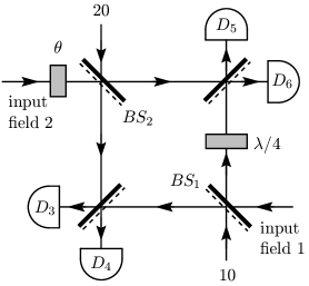
FIG. 1.: Eight-port homodyne detector with the four input ports 1, 10, 2, and 20 and four output ports with detectors $D_{3}$, $D_{4}$, $D_{5}$, and $D_{6}$ measuring the photon count differences $n_{43}=n_{4}-n_{3}$ and $n_{65}=n_{6}-n_{5}$. A quarter-wave plate causes a phase shift of $\pi/2$ in one arm of the interferometer. Input ports 10 and 20 remain open corresponding to a vacuum input. The input field 2 is phase shifted by an angle $\theta$. A measurement of photon count differences is made for each value of $\theta$.

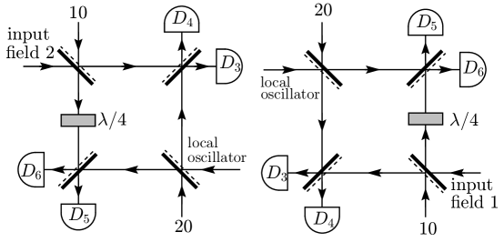
FIG. 2.: Indirect measurement scheme: A pair of eight-port homodyne detectors is used to measure the phase difference between the input fields 1 and 2. Each field is beat against a common strong local oscillator with coherent amplitude $\alpha$. Each eight-port detector has four detectors measuring the photon count differences $n_{43}$ and $n_{65}$. Two phase distributions are obtained and combined to give the phase distribution for the phase difference.

FIG. 3.: Comparison between phase distributions for both direct (solid line) and indirect measurement (dashed line), in the strong field limit. In this limit, the phase distribution of the direct scheme follows from Eq. (24), whereas for the indirect measurement, we have used the general expression Eq. (37). For both curves we have chosen the input fields 1 and 2 in coherent states with $\beta_{1}=1$ and $\beta_{2}=-4$.

REFERENCES

- [1] P. Carruters and M. M. Nieto, Rev. Mod. Phys. 40, 411 (1968); R. Lynch, Phys. Rep. 256, 367 (1995).
- [2] J. H. Shapiro, S. R. Shepard, and N. C. Wong, Phys. Rev. Lett. 62, 2377 (1989); A. S. Lane, S. L. Braunstein, and C. M. Caves, Phys. Rev. A 47, 1667 (1993); S. L. Braunstein and C. M. Caves, Phys. Rev. Lett. 72, 3439 (1994).
- [3] J. W. Noh, A. Fougères, and L. Mandel, Phys. Rev. Lett. 67, 1426 (1991); Phys. Rev. A 47, 4535 (1993).
- [4] J. W. Noh, A. Fougères, and L. Mandel, Phys. Rev. A 45, 424 (1992).
- [5] J. W. Noh, A. Fougères, and L. Mandel, Phys. Rev. A 46, 2840 (1992); Phys. Rev. Lett. 71, 2579 (1993).
- [6] J. W. Noh, A. Fougères, and L. Mandel, Phys. Rev. A 47, 4541 (1993); Phys. Rev. A 48, 1719 (1993); Phys. Scr. T48, 29 (1993), special issue on Quantum Phase and Phase Dependent Measurements, edited by W. P. Schleich and S. M. Barnett; A. Fougères, J. W. Noh, T. P. Grayson, and L. Mandel, Phys. Rev. A 49, 530 (1994); A. Fougères, J. R. Torgerson, and L. Mandel, Opt. Commun. 105, 199 (1994).
- [7] J. R. Torgerson and L. Mandel, Phys. Rev. Lett. 76, 3939 (1996).
- [8] Z. Hradil, Phys. Rev. A 47, 4532 (1993).
- [9] S. M. Barnett and D. T. Pegg, Phys. Rev. A 47, 4537 (1993); Z. Hradil and J. Bajer, Phys. Rev. A 48, 1717 (1993).
- [10] L. Mandel, in Foundations of Quantum Mechanics, edited by T. D. Black et al. (World Scientific, Singapore, 1992).
- [11] N. G. Walker and J. E. Caroll, Electron. Lett. 20, 981 (1984); N. G. Walker and J. E. Caroll, Opt. Quant. Electron. 18, 355 (1986).
- [12] M. Freyberger, K. Vogel, and W. P. Schleich, Phys. Lett. A 176, 41 (1993).
- [13] M. Freyberger and W. Schleich, Phys. Rev. A 47, R30 (1993).
- [14] M. Freyberger, K. Vogel, and W. Schleich, Quantum Opt. 5, 65 (1993).
- [15] S. L. Braunstein, Phys. Rev. A 42, 474 (1990).
- [16] W. Vogel and J. Grabow, Phys. Rev. A 47, 4227 (1993).