$\stackrel{{\scriptstyle\rm\textstyle DSF-1997/48}}{{\rm\textstyle quant-ph/9712028}}$
Quantum singular oscillator as a model of two-ion trap: an amplification of transition probabilities due to small time variations of the binding potential

Abstract

Following the paper by M. Combescure [Ann. Phys. (NY) 204, 113 (1990)], we apply the quantum singular time dependent oscillator model to describe the relative one dimensional motion of two ions in a trap. We argue that the model can be justified for low energy excited states with the quantum numbers $n\ll n_{max}\sim 100$, provided that the dimensionless constant characterizing the strength of the repulsive potential is large enough, $g_{*}\sim 10^{5}$. Time dependent Gaussian-like wave packets generalizing odd coherent states of the harmonic oscillator, and excitation number eigenstates are constructed. We show that the relative motion of the ions, in contradistinction to its center of mass counterpart, is extremely sensitive to the time dependence of the binding harmonic potential, since the large value of $g_{*}$ results in a significant amplification of the transition probabilities between energy eigenstate even for slow time variations of the frequency.

PACS: 03.65.Ge, 32.80.Pj, 33.80.Ps, 42.50.Dv

1 Introduction

A quantum system described by the singular oscillator Hamiltonian

$$\hat{H}=\frac{\hat{p}^{2}}{2\mu}+\frac{1}{2}\mu\omega^{2}(t)x^{2}+\frac{g}{x^{2}}$$ (1)

is one of rare examples admitting exact solutions of the Schrödinger equation. In the case of a constant frequency $\omega$, the eigenfunctions can be found in textbooks [1]. Generalizations of these eigenfunctions to the case of a time dependent frequency were obtained for the first time in [2]. Using these solutions, an exact propagator of the Schrödinger equation with Hamiltonian (1) was found in [3]. An elegant method of calculating propagators of time dependent quantum systems, including (1), on the basis of quantum operator integrals of motion, was developed in [4]. The same propagator was obtained in the framework of the path integrals approach in [5] (a constant frequency) and [6] (a time dependent frequency). A detailed analysis of solutions found in [2] was performed in Ref. [7], where two families of time dependent wave packets generalizing coherent states of the harmonic oscillator [8] were also constructed. An asymmetrical singular nonstationary oscillator in two and three dimensions was considered in [9] (see also [10] for the stationary case). A systematic study of wave packets and coherent states in the centrifugal and other anharmonic potentials was given in [11].

The exact solvability of the Schrödinger equation with Hamiltonian (1) is explained by the fact that this Hamiltonian is a linear combination of three generators of the $su(1,1)$ algebra,

$$\frac{p^{2}}{2\mu}+\frac{g}{x^{2}},\quad x^{2},\quad xp+px.$$ (2)

The propagator and solutions of the Schrödinger equation with a generic Hamiltonian, which is a linear combination of generators (2) with arbitrary time dependent coefficients, were found in [12] (see also [13, 14], where other representations of the $su(1,1)$ algebra were considered). The universal invariants and generalized uncertainty relations for this generic case were studied in [15]. A special case of periodic time dependent coefficients, including the adiabatic (Berry’s phase) and delta-kicked limits, was considered in [16]. Recently, many results obtained in the cited papers were rediscovered, see e.g. [17, 18, 19].

A distinguished role of Hamiltonian (1) is explained by the fact that, in a sense, it belongs to a boundary between linear and nonlinear problems of classical and quantum mechanics. For this reason, it was used in many applications. For example, it served as an initial point in constructing interesting exactly solvable models of interacting $N$-body systems [20]. It was used also for modelling diatomic [12] and polyatomic [21] molecules, and for the evaluation of the accuracy of the quasiclassical approximation for nonquadratic Hamiltonians [22]. Studying the limiting case $g=0$ of the generalized coherent states of a singular oscillator led to introducing a concept of even and odd coherent states [7], which are considered nowadays as simplest models of quantum macroscopic superpositions — the so called Schrödinger cat states [23].

Even and odd coherent states of photons were created in cavity experiments [24]. Another superposition of coherent states of the Schrödinger cat type, similar to even and odd coherent states, can be created from an initial coherent state in a nonlinear Kerr medium [25]. This superposition has the same Poisson quantum number distribution function as the usual coherent state, so it is “more classical” [26] than even and odd coherent states, which have highly oscillating quantum number distribution functions (strong oscillations of photon distribution functions, like in squeezed states [27, 28], are believed to be a characteristics of nonclassical states [29]). The photon statistics of parametrically excited even and odd coherent states (which are superpositions of squeezed states) was discussed in [30]. A quantum sling mechanism of constructing squeezed and correlated states from usual coherent states was suggested in [31].

Unfortunately, photon nonclassical states are very sensitive to the interaction with an environment, and decoherence phenomena may destroy the specific interference pattern of the Schrödinger cat superposition states very rapidly (for example, an increase of temperature leads to a decrease of oscillations of the photon distribution function in squeezed and correlated states [32]). Much more stable even and odd coherent states can be created for trapped ions (for example, in the Paul trap [33]), as was demonstrated both theoretically [34, 35] and experimentally [36]. Different aspects of quantum motion of ions in traps were discussed, e.g. in [26, 37, 38]. In particular, various nonlinear modifications of coherent states [39] could be created for trapped ions [40].

Here we wish to show that the limiting case of very large values of the dimensionless parameter $\mu g/\hbar^{2}$ is also interesting, because it may have some relation to the problem of the relative motion of ions in electromagnetic traps. Indeed, the ions in the Paul or Penning traps move in time dependent harmonic potentials, and the stable configurations correspond under certain conditions to an effectively unidimensional motion along the trap axis [41]. In such a case, a relative motion of two ions can be described as the motion of a single particle (with the reduced mass) in the Coulomb repulsive potential $V(x)=e^{2}/x$. Combescure [42] proposed to replace the real Coulomb potential by the singular oscillator potential $V_{ef}=g/x^{2}$. Using the solutions of the Schrödinger equation in the same form as in [2, 7] and considering the harmonic time dependence of the frequency $\omega(t)$, he made some qualitative conclusions concerning the relative motion of the ions in the Paul trap. However, he did not give any estimations which could justify his model. The aim of our article is to provide such a justification for large values of parameter $g$, and to consider specific features of solutions in this special case, stressing qualitative differences between the relative and center of mass motions. We shall demonstrate that the transition probabilities between energy eigenstates of the relative motion are significantly amplified in comparison with that of the center of mass motion, even when time variations of the frequency are very small. This result may be interpreted as an indication to a high sensitivity of the relative ion motion to small time variations of the binding trap potential, which could result in some kind of a chaotic behaviour in the case of the real Coulomb interaction potential [41, 43, 44]. Note that an irregular (although not chaotic, in the strict sense of this notion) behaviour of time dependent linear quantum systems described by $su(1,1)$ invariant Hamiltonians with (quasi)periodic $\delta$-kicked coefficients was studied in [45, 46] (see also [47]).

2 Justification of the model

Let us compare two potentials ($\mu$ is the reduced mass of two ions),

$$V(x)=\frac{1}{2}\mu\omega^{2}x^{2}+\frac{e^{2}}{x},$$ (3)

$$V_{g}(x)=\frac{1}{2}\mu\omega_{g}^{2}x^{2}+\frac{g}{x^{2}}.$$ (4)

If the energy of a particle is not too large (as in real traps, where ions are cooled), then it performs small oscillations near the equilibrium coordinates satisfying the equations $V^{\prime}(x)=0$ and $V^{\prime}_{g}(x)=0$, namely,

$$x_{e}=\left(\frac{e^{2}}{\mu\omega^{2}}\right)^{1/3},\quad x_{g}=\left(\frac{2g}{\mu\omega_{g}^{2}}\right)^{1/4}.$$

The frequencies of oscillations are determined by the second derivatives of the potentials in the equilibrium points,

$$\Omega_{e,g}=\sqrt{V^{\prime\prime}\left(x_{e,g}\right)/\mu},\quad\Omega_{e}=\sqrt{3}\omega,\quad\Omega_{g}=2\omega_{g}.$$

Demanding the equilibrium positions and the effective frequencies of the real potential, (3), and its simulation, (4), to coincide , we obtain the following parameters of the effective potential describing the relative ion motion:

$$\omega_{g}=\frac{\sqrt{3}}{2}\omega,\quad g=\frac{3}{8}\left(\frac{e^{8}}{\mu\omega^{2}}\right)^{1/3}.$$ (5)

The minimum is twice less than that of the real potential,

$$V\left(x_{e}\right)=\frac{3}{2}\mu\omega^{2}x_{e}^{2},\quad V_{g}\left(x_{g}\right)=\mu\omega_{g}^{2}x_{g}^{2}=\frac{1}{2}V\left(x_{e}\right),$$

but this shift seems not important.

The solutions of the Schrödinger equation depend on the dimensionless parameter

$$g*=2\mu g/\hbar^{2}.$$ (6)

Taking the $x$-dependent part of the trap potential energy as $V_{t}(x)=eUx^{2}/(2L^{2})$, $U$ being the voltage applied to the cap electrodes separated by the distance $2L$, we have $\omega^{2}=eU/(2\mu L^{2})$ (since $\mu=m_{i}/2$, where $m_{i}$ is the ion mass). Therefore,

$$g_{*}=\frac{3}{4}\left(\frac{\mu^{2}e^{8}}{\hbar^{6}\omega^{2}}\right)^{1/3}=\frac{3\mu}{4m}\left[\frac{4\mbox{Ry}}{eU}\left(\frac{L}{a_{B}}\right)^{2}\right]^{1/3},$$ (7)

where $m$ is the electron mass, Ry is the Rydberg constant, and $a_{B}$ is Bohr’s radius. For typical trap parameters, $\mu/m\sim 10^{5}$, $U\sim 100$ V, $L\sim 1$ mm, we have $g_{*}\sim 10^{10}$.

A specific feature of the singular oscillator potential is the equidistant character of the energy spectrum. Since the real interaction potential does not possess such a property, the replacement of (3) by (4) can be justified, provided that the corrections to the energy spectrum due to the anharmonicity of the potential (3) are small, comparing with the effective oscillator energy difference $\hbar\Omega_{e}=\sqrt{3}\hbar\omega$. The cubic anharmonic correction to the potential (3) in the vicinity of the equilibrium point is $-\left(e^{2}/x_{e}^{4}\right)(\delta x)^{3}$, $\delta x$ being a small deviation from the equilibrium position $x_{e}$. Assuming $\mu\Omega_{e}^{2}(\delta x)^{2}=n\hbar\Omega_{e}$ for the $n$th excited effective harmonic oscillator energy level, one can verify that the anharmonic corrections can be neglected under the condition

$$n\ll n_{max}\sim 3\left(\frac{\mu e^{4}}{\hbar^{3}\omega}\right)^{1/9}\sim 3g_{*}^{1/6}.$$ (8)

For the same trap parameters as above, $n_{max}\approx 100$. Consequently, the singular oscillator model can be applied for describing the low energy excited states of the relative ion motion.

3 Time dependent solutions for a large repulsive constant

A complete set of orthonormalized solutions to the Schrödinger equation with Hamiltonian (1) can be chosen in the form [2, 7]

$$\Psi_{n}(x,t)=\left[2\left(\frac{\mu}{\hbar\epsilon^{2}}\right)^{d+1}\frac{n!}{\Gamma(d+n+1)}\right]^{\frac{1}{2}}\left(\frac{\epsilon^{*}}{\epsilon}\right)^{n}x^{d+\frac{1}{2}}\exp{\left(\frac{i\mu\dot{\epsilon}}{2\hbar\epsilon}x^{2}\right)}L^{d}_{n}\left(\frac{\mu x^{2}}{\hbar|\epsilon|^{2}}\right),$$ (9)

where $d=\frac{1}{2}\sqrt{1+4g_{*}}$, and $L^{d}_{n}(z)$ is an associated Laguerre polynomial. (Hereafter we write $\omega$ instead of $\omega_{g}$, assuming that the frequency rescaling has been done.) The time dependent complex function $\epsilon(t)$ is a special solution to the classical harmonic oscillator equation,

$$\ddot{\epsilon}+\omega^{2}(t)\epsilon=0,$$ (10)

satisfying the normalization condition

$$\dot{\epsilon}\epsilon^{*}-\dot{\epsilon}^{*}\epsilon=2i.$$ (11)

If $\omega=const$, the solutions (9) go to the energy eigenstates, provided that function $\epsilon(t)$ is chosen as $\epsilon(t)=\omega^{-1/2}\exp\left(i\omega t\right)$.

Expression (9) is written for $x>0$. Its continuation to the negative semiaxis (since $x$ is the relative coordinate of two ions along the trap symmetry axis, it can be both positive and negative) depends on the symmetry properties of the two-particle wavefunction determined by the kind of statistics (Bose or Fermi, if the ions are identical), so that one should write $\Psi(x)=\pm\Psi(-x)$ for $x<0$. There are no problems with the continuity of the solutions or their derivatives at $x=0$, provided that $d>1/2$ (i.e. $g>0$). Extending the wave function to the whole axis, one must only change the normalization by the evident factor $\sqrt{2}$. Authors of the recent paper [48] claimed that there is a nontrivial influence of the parameter $d$ on the possibility of existence of the bound states of two ions in the Paul trap, depending on the type of quantum statistics. However, this conclusion was a consequence of incorrect manipulations with the expressions for the wave function at $x>0$ and $x<0$, which resulted in the coordinate independent factor $1\pm\cos(d+1/2)\pi$ in the wave function. This factor turns into zero for specific values of parameter $d$, which was interpreted by the authors of [48] as a disappearance of bound states. They forgot, however, to normalize the wave function. If they did this, then the incorrect factor would disappear, not the bound states.

Solution (9) is an eigenfunction of the time dependent integral of motion (a generalization of the harmonic oscillator number operator)

$$\hat{B}=\frac{1}{\hbar}\left[|\epsilon|^{2}\left(\frac{\hat{p}^{2}}{2\mu}+\frac{g}{x^{2}}\right)+\frac{\mu}{2}|\dot{\epsilon}|^{2}x^{2}-\frac{1}{2}\mbox{Re}\left(\dot{\epsilon}\epsilon^{*}\right)\left(\hat{x}\hat{p}+\hat{p}\hat{x}\right)\right],$$ (12)

with an eigenvalue $2n+d+1$. There exists another integral of motion [7],

$$\hat{A}=\frac{1}{2\mu\hbar}\left[\left(\epsilon\hat{p}-\dot{\epsilon}\mu\hat{x}\right)^{2}+2\epsilon^{2}\frac{\mu g}{x^{2}}\right],$$ (13)

which is a generalization of the square of the harmonic oscillator annihilation operator $\hat{a}^{2}$. A normalized eigenstate of operator (13), $\hat{A}|\alpha\rangle=\alpha^{2}|\alpha\rangle$ ($\alpha$ being an arbitrary complex number), reads [7]

$$\langle x|\alpha\rangle = \frac{|\alpha|^{d}}{\sqrt{2^{d}I_{d}\left(|\alpha|^{2}\right)}}\sum_{n=0}^{\infty}\frac{\alpha^{2n}}{\sqrt{2^{2n}n!\Gamma(n+d+1)}}\Psi_{n}(x,t)$$ (14)

$$= \left[\frac{2\mu x}{\hbar\epsilon^{2}I_{d}\left(|\alpha|^{2}\right)}\right]^{1/2}\left(\frac{|\alpha|}{\alpha}\right)^{d}\exp\left(\frac{i\mu\dot{\epsilon}}{2\hbar\epsilon}x^{2}+\frac{\epsilon^{*}}{2\epsilon}\alpha^{2}\right)J_{d}\left(\frac{x\alpha}{\epsilon}\sqrt{\frac{2\mu}{\hbar}}\right),$$ (15)

where $J_{d}(x)$ and $I_{d}(x)$ are the Bessel function and the modified Bessel function, respectively. Similar (time independent) eigenstates of the lowering generator of an abstract $su(1,1)$ algebra in another specific representation were considered by Barut and Girardello [50]. Various generalizations and concrete realizations of these states were discussed, e.g. in [51, 52, 53, 54], where many references to other publications can be found.

Taking $d=1/2$ (i.e. $g=0$) and replacing the reduced mass, $\mu$, by the total mass of two ions, $M$, we arrive at the expressions for the wave functions describing the odd states of the center of mass motion in the harmonic potential with frequency $\omega$ (remember, however, that the frequency of small oscillations of the relative distance between ions is $\sqrt{3}$ times higher than the frequency of the center of mass motion). The even wave functions of the center of mass motion are obtained by means of a formal substitution $d=-1/2$.

The time dependences of the mean values of the operators (2) in any state are as follows,

$$\langle x^{2}\rangle = \frac{\hbar}{m}\left[|\epsilon|^{2}\langle\hat{B}\rangle-\mbox{Re}\left(\epsilon^{2}\langle\hat{A}^{{\dagger}}\rangle\right)\right],$$ (16)

$$\left\langle\frac{\hat{p}^{2}}{2\mu}+\frac{g}{x^{2}}\right\rangle = \frac{\hbar}{2}\left[|\dot{\epsilon}|^{2}\langle\hat{B}\rangle-\mbox{Re}\left(\dot{\epsilon}^{2}\langle\hat{A}^{{\dagger}}\rangle\right)\right],$$ (17)

$$\left\langle\hat{x}\hat{p}+\hat{p}\hat{x}\right\rangle = 2\hbar\left[\mbox{Re}\left(\dot{\epsilon}\epsilon^{*}\right)\langle\hat{B}\rangle-\mbox{Re}\left(\dot{\epsilon}\epsilon\langle\hat{A}^{{\dagger}}\rangle\right)\right].$$ (18)

In particular, the mean value of the operator $\hat{B}$ in the state (15) equals [7]

$$\langle\alpha|\hat{B}|\alpha\rangle=1+|\alpha|^{2}\frac{I^{\prime}_{d}\left(|\alpha|^{2}\right)}{I_{d}\left(|\alpha|^{2}\right)}.$$ (19)

Formulas (15) and (19) can be simplified for large values of coefficient $d$. Taking into account the asymptotics of the Bessel functions of a large index [49],

$$\sqrt{2\pi}I_{d}(z)\approx\left(d^{2}+z^{2}\right)^{-1/4}\exp\left[\sqrt{d^{2}+z^{2}}+d\ln\left(\frac{z}{z+\sqrt{d^{2}+z^{2}}}\right)\right],\quad d\gg 1,\quad d>z.$$ (20)

and calculating the power series expansion of the exponential argument in (20) up to $z^{4}$ terms, we obtain

$$\langle\alpha|\hat{B}|\alpha\rangle=1+d+\frac{|\alpha|^{4}}{2d}.$$ (21)

Consequently, the energy difference between the states $|\alpha\rangle$ and $|0\rangle$ becomes noticeable only for $|\alpha|^{4}\sim d$. In such a case, due to Eq. (16), the mean value $\langle x^{2}\rangle$ oscillates in the vicinity of the average position $\langle x_{0}^{2}\rangle=(\hbar/m)|\epsilon|^{2}\langle\hat{B}\rangle\sim 2$, the amplitude of oscillations being of an order of $\sqrt{d}\ll d$. For this reason, we can simplify formula (15), replacing the Bessel function by its asymptotical form following from (20) and expanding the arising exponential argument up to the terms of the order of $|\alpha|^{4}/d$ or $x^{2}|\alpha|^{2}/d$. After some algebra, we obtain the expression

$$\langle x|\alpha\rangle = (2\pi d)^{-1/4}\left(\frac{2\mu x}{\hbar\epsilon^{2}}\right)^{1/2}\left(\frac{\epsilon^{*}}{\epsilon}\right)^{d/2}\exp\left[-\frac{\mu^{2}y^{2}}{4\hbar^{2}|\epsilon|^{4}d}+\frac{i\mu}{2\hbar}\mbox{Re}\left(\frac{\dot{\epsilon}}{\epsilon}\right)y-\frac{|\alpha|^{4}}{8d}\right.$$ (22)

$$-\left.\frac{\alpha^{4}\epsilon^{*2}}{8d\epsilon^{2}}-\frac{\alpha^{2}y}{2\epsilon^{2}d}\right],$$

where

$$y(x,t)=x^{2}-\frac{\hbar}{\mu}|\epsilon|^{2}(d+1).$$ (23)

In the right hand side of Eq. (22) we recognize the generating function of the Hermite polynomials [49],

$$\exp\left(-z^{2}+2zx\right)=\sum_{n=0}^{\infty}\frac{z^{n}}{n!}H_{n}(x).$$

Comparing it with the expansion (14) and using Stirling’s formula, we arrive at the following asymptotical expression:

$$\Psi_{n}(x,t)=(2\pi d)^{-1/4}\left(\frac{2\mu x}{\hbar\epsilon^{2}2^{n}n!}\right)^{1/2}\left(\frac{\epsilon^{*}}{\epsilon}\right)^{n+d/2}\exp\left[-\frac{\mu^{2}y^{2}}{4\hbar^{2}|\epsilon|^{4}d}+\frac{i\mu}{2\hbar}\mbox{Re}\left(\frac{\dot{\epsilon}}{\epsilon}\right)y\right]H_{n}\left(-\frac{\mu y}{\sqrt{2d}\hbar|\epsilon|^{2}}\right).$$ (24)

The probability density in the state (22) is Gaussian, but with respect to variable $x^{2}$:

$$|\langle x|\alpha\rangle|^{2}=(2\pi d)^{-1/2}\frac{2\mu x}{\hbar|\epsilon|^{2}}\exp\left[-\frac{\mu^{2}\left(x^{2}-\langle\alpha|x^{2}|\alpha\rangle\right)^{2}}{2\hbar^{2}|\epsilon|^{4}d}\right],$$ (25)

$$\langle\alpha|x^{2}|\alpha\rangle=\frac{\hbar}{m}\left[|\epsilon|^{2}\left(1+d+\frac{|\alpha|^{4}}{2d}\right)-\mbox{Re}\left(\epsilon^{*2}\alpha^{2}\right)\right].$$ (26)

Exact solutions to the Schrödinger equation in the form of the power-Gaussian wave packets were constructed in [2, 7]. From the modern point of view, these packets can be considered as generalizations of the odd squeezed states (in the context of an abstract $su(1,1)$-invariant Hamiltonian similar states were considered, e.g. in [55]; recent results and other references can be found in [53, 54]):

$$|z\rangle = \left(1-|z|^{2}\right)^{\frac{d+1}{2}}\exp\left(\frac{z}{2}\hat{A}^{{\dagger}}\right)|0\rangle$$ (27)

$$= \left[\frac{2\mu x}{\hbar\Gamma(d+1)}\right]^{1/2}\left(\frac{\mu x^{2}}{\hbar}\right)^{d/2}\left(\frac{\sqrt{1-|z|^{2}}}{\epsilon-z\epsilon^{*}}\right)^{d+1}\exp\left[\frac{i\mu}{2\hbar}\frac{\dot{\epsilon}-z\dot{\epsilon}^{*}}{\epsilon-z\epsilon^{*}}x^{2}\right].$$ (28)

For not too large values of $d$, the states (15) and (28) are obviously different. However, for $d\gg 1$ and moderate values of $x$, $\alpha$, and $z$, the function $|\langle x|z\rangle|^{2}$ is given by the same expression (25). The only difference is in the formula for the mean value of $x^{2}$:

$$\langle z|x^{2}|z\rangle=(d+1)\frac{\hbar}{m}\frac{|\epsilon-z\epsilon^{*}|^{2}}{1-|z|^{2}}\approx(d+1)\frac{\hbar}{m}\left[|\epsilon|^{2}\left(1+2|z|^{2}\right)-\mbox{Re}\left(\epsilon^{2}z^{*}\right)\right].$$ (29)

For moderately excited states, parameter $z$ must be small, since [7]

$$\langle z|\hat{B}|z\rangle=(d+1)\frac{1+|z|^{2}}{1-|z|^{2}}.$$

Note that the relative width of the distributions given by Eqs. (24) and (25) practically does not depend on time, $\Delta y/y_{max}\sim\left(|\epsilon|^{2}\sqrt{d}\right)/\left(|\epsilon|^{2}d\right)\sim 1/\sqrt{d}$, while the position of the center of the distribution, $y_{max}$, may vary essentially even with small variations of function $|\epsilon|^{2}$, due to the large value of $d$. As a consequence, the covering between the packets taken at different moments of time may be very small even for weak variations of the frequency $\omega(t)$, resulting in the effect of the amplification of transition probabilities, discussed in the next section.

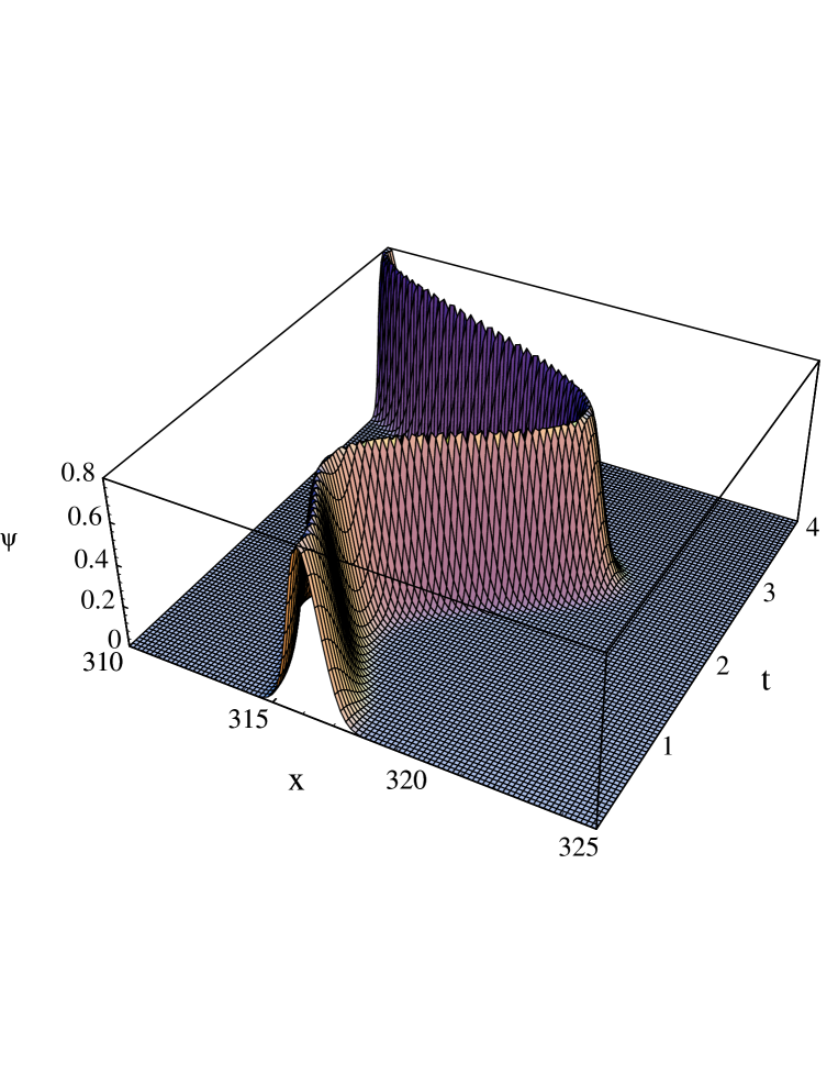
Figure 1: $|\Psi_{0}(x,t)|^{2}$ for $d=10^{5}$ and $k=0.02$ ($x$ and $t$ are dimensionless).

In Fig.1 and 2 we plot the probability densities for the states $\Psi_{0}(x,t)$ and $\Psi_{2}(x,t)$ (24) in the parametric resonance case (using dimensionless units)

$$\omega^{2}(t)=\frac{1+k\cos{2t}}{1+k},~{}~{}k\ll 1,$$ (30)

when an explicit analytical (approximate) expression for $\epsilon(t)$ reads [30],

$$\epsilon(t)=\cosh{\frac{kt}{4}}e^{it}-i\sinh{\frac{kt}{4}}e^{-it}.$$ (31)

We assume $d=10^{5}$ and $k=0.02$.

4 Amplification of transition probabilities

Suppose that the frequency $\omega(t)$ assumes constant values, $\omega_{i}$ and $\omega_{f}$, in the remote past and future, respectively (such a situation corresponds to the Penning trap, when the voltage between electrodes exhibits some time variations), and that the singular oscillator was in the $n$th stationary state at $t\to-\infty$. This state is given by Eq. (9) with $\epsilon_{i}(t)=\omega_{i}^{-1/2}\exp\left(i\omega_{i}t\right)$. The asymptotical form of the solution to Eq. (10) at $t\to\infty$ reads

$$\epsilon(t\to\infty)=\omega_{f}^{-1/2}\left[\xi\exp\left(i\omega_{f}t\right)-\eta\exp\left(-i\omega_{f}t\right)\right],$$

$\xi$ and $\eta$ being constant complex coefficients satisfying the restriction $|\xi|^{2}-|\eta|^{2}=1$, following from (11). The transition probability from the initial $n$th energy eigenstate to the final $m$th one (corresponding to frequency $\omega_{f}$) was found in [7]:

$$W_{n}^{m}=\frac{\mu_{mn}!\Gamma\left(\nu_{mn}+d+1\right)}{\nu_{mn}!\Gamma\left(\mu_{mn}+d+1\right)}r^{|m-n|}(1-r)^{d+1}\left[P_{\mu_{mn}}^{(|m-n|,d)}(1-2r)\right]^{2}$$ (32)

$$=\frac{\nu_{mn}!\Gamma\left(\nu_{mn}+d+1\right)r^{|m-n|}(1-r)^{d+1}}{\mu_{mn}!\Gamma\left(\mu_{mn}+d+1\right)[|m-n|!]^{2}}\left[F\left(-\mu_{mn},\nu_{mn}+d+1;|m-n|+1;r\right)\right]^{2}.$$ (33)

Here $\mu_{mn}\equiv\mbox{min}(m,n)$, $\nu_{mn}\equiv\mbox{max}(m,n)$, $\Gamma(z)$ is the Gamma function, $P_{n}^{(\alpha,\beta)}(z)$ is the Jacobi polynomial, $F(a,b;c;z)$ is the Gauss hypergeometric function [49], and $r\equiv|\eta/\xi|^{2}$ is a reflection coefficient from an effective potential barrier determined by the time dependence of $\omega^{2}(t)$. In particular, the ground state excitation probability equals

$$W_{0}^{m}=\frac{\Gamma\left(m+d+1\right)}{m!\Gamma\left(d+1\right)}r^{m}(1-r)^{d+1}.$$ (34)

In the special cases of $d=\pm 1/2$ (describing the center of mass motion in the pure harmonic time dependent potential), one can use the quadratic transformation of the Gauss hypergeometric function [49],

$$F(a,b;a+b+1/2;4z(1-z))=F(2a,2b;a+b+1/2;z),$$

to reproduce the known formula for the transition probabilities between the energy levels of the harmonic oscillator with a time dependent frequency [56] (see also [57] for details and the bibliography),

$$W_{k}^{j}=\frac{k!j!r^{|k-j|/2}\sqrt{1-r}}{2^{|k-j|}\left([(k+j)/2]!\right)^{2}}\left[P_{\mu_{kj}}^{(|k-j|/2\,,\,|k-j|/2)}\left(\sqrt{1-r}\right)\right]^{2}.$$ (35)

Here $k$ and $j$ must have the same parity.

Now we have to take into account that coefficient $d$ is very large, $d\approx\sqrt{g_{*}}\sim 10^{5}$, in the case of the relative ion motion, while quantum numbers $m$ and $n$ must be much less than $100$. In such a case, using an approximation $(b)_{k}\equiv b(b+1)\ldots(b+k-1)\approx b^{k}$, $b\gg 1$, we can reduce the Gauss hypergeometric function

$$F(a,b;c;z)\equiv\sum_{k=0}^{\infty}\frac{(a)_{k}(b)_{k}}{(c)_{k}k!}z^{k}$$

to the confluent hypergeometric function

$$\Phi(a;c;bz)\equiv\sum_{k=0}^{\infty}\frac{(a)_{k}}{(c)_{k}k!}(bz)^{k}.$$

With the same accuracy, we can write $\Gamma(d+n)\approx\Gamma(d)d^{n}$. Then Eq. (33), together with the relation between the confluent hypergeometric function and the Laguerre polynomial [49],

$$\Phi(-n;c+1;z)\equiv\frac{n!}{(c+1)_{n}}L_{n}^{c}(z),$$

lead to a simplified form of the transition probability for $d\gg 1$:

$$W_{n}^{m}=\frac{\mu_{mn}!}{\nu_{mn}!}(rd)^{|m-n|}(1-r)^{d+1}\left[L_{\mu_{mn}}^{|m-n|}(rd)\right]^{2},$$ (36)

$$W_{0}^{m}=\frac{(rd)^{m}}{m!}(1-r)^{d+1}.$$ (37)

If the frequency variation is small, for instance, adiabatic, then the effective reflection coefficient $r$ is small too (excluding the case of the parametric resonance). In this case, the Taylor expansion of formula (33) yields

$$W_{n}^{m}=\frac{\nu_{mn}\Gamma\left(\nu_{mn}+d+1\right)}{\mu_{mn}\Gamma\left(\mu_{mn}+d+1\right)}\frac{r^{|m-n|}}{[|m-n|!]^{2}}\left[1-\frac{2mn+(d+1)(m+n+1)}{|m-n|+1}r+\cdots\right].$$ (38)

Consequently, if $r\ll 1$, and quantum numbers $m,n$ are not too large, the transition probabilities of the center of mass motion ($d=\pm 1/2$) are suppressed by the factor $r^{|m-n|}$. However, this may not be true for the relative motion, since the reflection coefficient is effectively amplified by the large factor $d$. This is seen distinctly from the special form of formula (36), which is valid for $r^{2}d\ll 1$:

$$W_{n}^{m}=\frac{\mu_{mn}!}{\nu_{mn}!}(rd)^{|m-n|}e^{-rd}\left[L_{\mu_{mn}}^{|m-n|}(rd)\right]^{2}.$$ (39)

Fig.3 gives the dependence of $W_{n}^{m}$ on the product $rd$ for $n=5$ and $m=0,2,5,10$. The surface plots of the relative motion transition probabilities $W_{n}^{m}$ for a fixed value of $d=10^{5}$, and for $r=10^{-6},10^{-5},10^{-4}$ are given in Figs.4, 5, and 6, respectively. Fig.4 shows that actually there is no transitions to other states, if $rd=0.1$, and $m,~{}n\leq 5$, while for larger values of $m,~{}n$ some structure appears in the plot. This structure becomes more complicated, when $rd=1$. For $rd=10$, the picture is quite different from the adiabatic behavior, although coefficient $r$ is still very small.

If $rd\gg m,n\sim 1$, then the leading term of the Laguerre polynomial in (39) yields

$$W_{n}^{m}=\frac{(rd)^{m+n}}{m!n!}(1-r)^{d+1}\approx\frac{(rd)^{m+n}}{m!n!}e^{-rd}.$$ (40)

Eq. (40) clearly shows, that for moderate values of $m,n\ll rd$ (when the model considered can be justified), all transition probabilities are negligibly small. This means that even small time variations of the binding trap harmonic potential result in the excitation of the states with high values of the relative motion energy, while the quantum state of the centre of mass motion is practically unchanged under the same conditions. This phenomenon can be interpreted as an indication of an instability of the relative ion motion with respect to small perturbations in the quantum regime. We should note, however, that the quantitative calculations of the transition probabilities to highly excited states of the relative motion of real ions cannot be performed in the framework of the singular oscillator potential model, since the condition (8) is not fulfilled for these states.

5 Conclusions

The main results of the paper can be summarized as follows. We have presented new asymptotical forms of the wave packets of the time dependent singular quantum oscillator in the case of a very strong repulsive centrifugal potential. We have shown that such a potential can approximate to a certain extent the real Coulomb repulsion between two ions in a trap. We have found an extreme sensitivity of the transition amplitudes between energy eigenstates to small variations of the coefficients of the Hamiltonian. It is worth noticing in this regard that the system of two trapped ions interacting via the true Coulomb potential exhibits under certain conditions a chaotic behaviour [41, 43, 44]. Of course, one cannot expect any chaos, in the strict sense of this word, in the framework of the one-dimensional exactly solvable model. Nonetheless, our results might be interpreted as an indication of a possible irregular behaviour (which manifests itself just in a high sensitivity to small changes of the initial conditions of parameters describing the system), if one replaces the exactly solvable potential by the realistic one (which cannot be treated analytically).

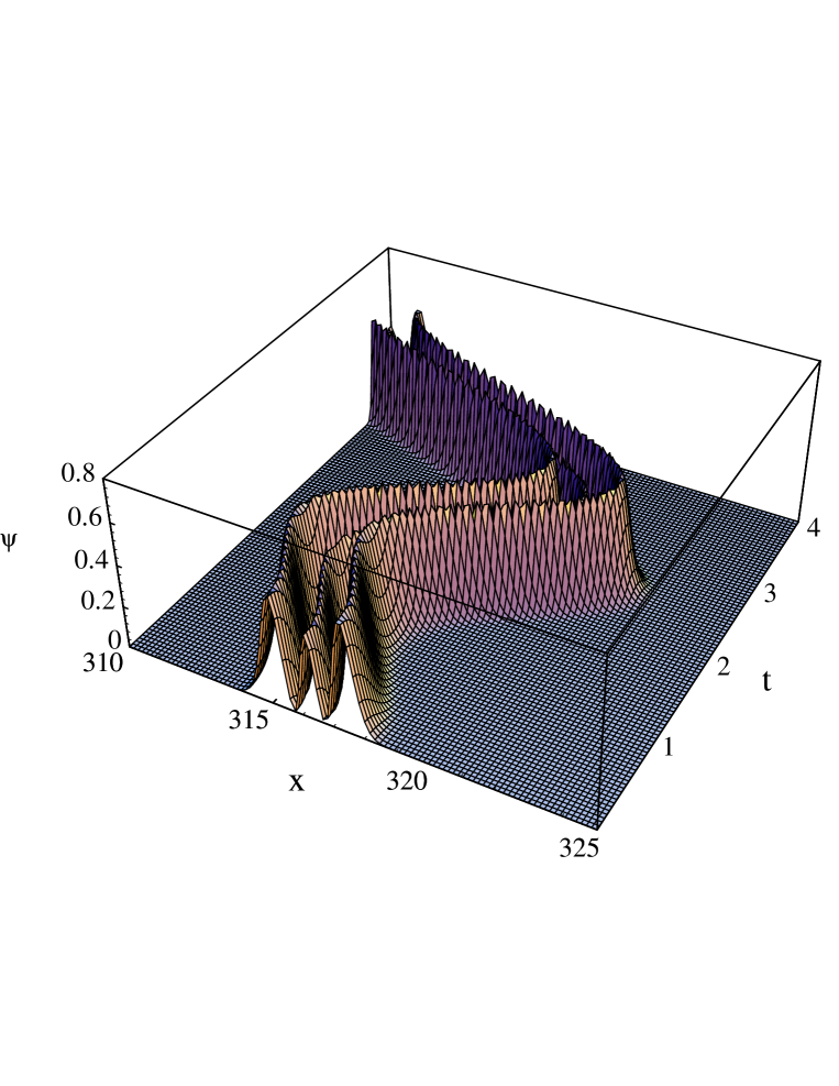
Figure 2: $|\Psi_{2}(x,t)|^{2}$ for $d=10^{5}$ and $k=0.02$ ($x$ and $t$ are dimensionless).

Figure 3: $W_{5}^{m}(rd)$ for $m=0,2,5,10$ ( $r$ and $d$ are dimensionless).

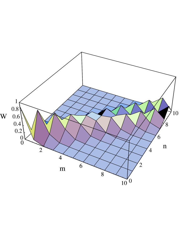
Figure 4: $W_{n}^{m}$ for $d=10^{5}$ and $r=10^{-6}$

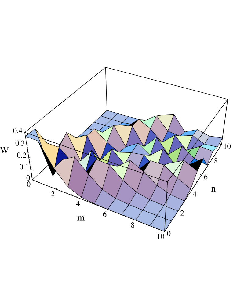
Figure 5: $W_{n}^{m}$ for $d=10^{5}$ and $r=10^{-5}$

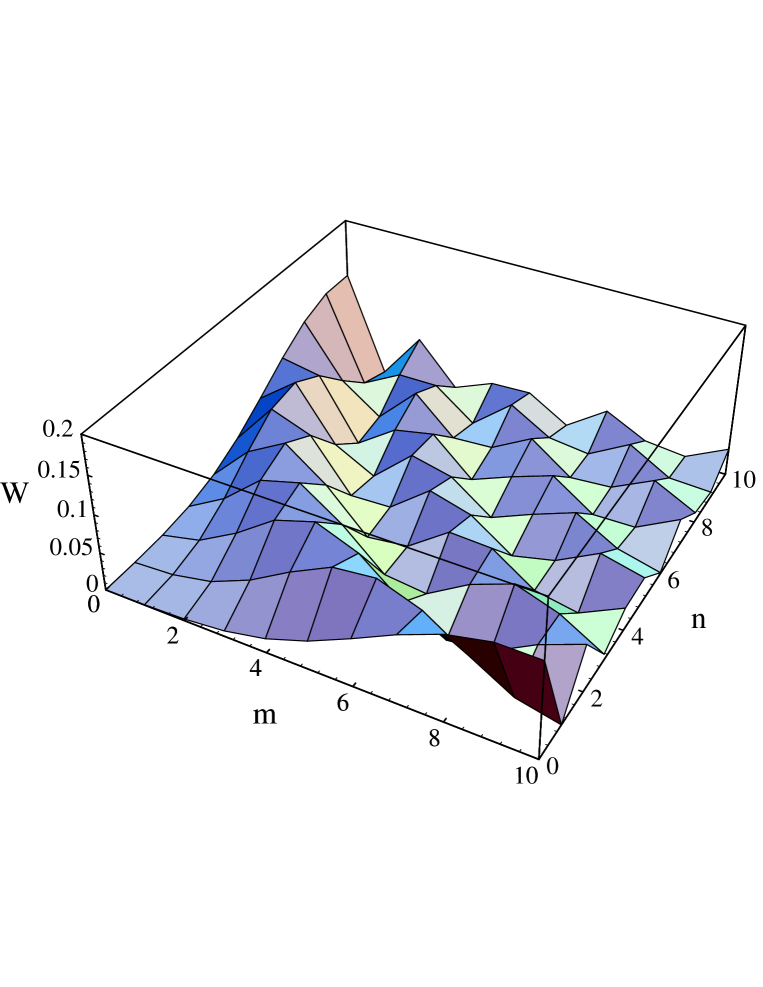
Figure 6: $W_{n}^{m}$ for $d=10^{5}$ and $r=10^{-4}$

References

- [1] L. D. Landau and E. M. Lifshitz, Quantum Mechanics (Addison-Wesley, Reading, 1965).
- [2] P. Camiz, A. Gerardi, C. Marchioro, E. Presutti, and E. Scacciatelli, J. Math. Phys. 12, 2040 (1971).
- [3] V. V. Dodonov, I. A. Malkin, and V. I. Man’ko, Phys. Lett. A 39, 377 (1972).
- [4] V. V. Dodonov, I. A. Malkin, and V. I. Man’ko, Int. J. Theor. Phys. 14, 37 (1975); Teor. Mat. Fiz. 24, 164 (1975) [Sov. Phys. - Theor. & Math. Phys. 24, 746 (1975)].
- [5] D. Peak and A. Inomata, J. Math. Phys. 10, 1422 (1969).
- [6] D. C. Khandekar and S. V. Lawande, J. Math. Phys. 16, 384 (1975).
- [7] V. V. Dodonov, I. A. Malkin, and V. I. Man’ko, Physica 72, 597 (1974).
- [8] R.J. Glauber, Phys. Rev. Lett. 10, 84 (1963).
- [9] V. V. Dodonov, I. A. Malkin, and V. I. Man’ko, Nuovo Cim. B 24, 46 (1974).
- [10] A. Hautot, J. Math. Phys. 14, 1320 (1973).
- [11] M. M. Nieto and L. M. Simmons, Jr., Phys. Rev. D 20, 1321, 1332, 1342 (1979).
- [12] S. M. Chumakov, V. V. Dodonov, and V. I. Man’ko, J. Phys. A 19, 3229 (1986).
- [13] S. V. Prants, J. Phys. A 19, 3457 (1986).
- [14] G. Dattoli, S. Solimeno, and A. Torre, Phys. Rev. A 34, 2646 (1986).
- [15] V. V. Dodonov and V. I. Man’ko, in Group Theoretical Methods in Physics, Proceedings of the Second International Seminar, Zvenigorod, 24-26 November 1982, edited by M. A. Markov, V. I. Man’ko, and A. E. Shabad (Harwood Academic Publishers, Chur–London–New York, 1985), Vol. 1, p. 591.
- [16] V. V. Dodonov, V. I. Man’ko, and D. V. Zhivotchenko, Nuovo Cim. B 108, 1349 (1993).
- [17] G. S. Agarwal and S. Chaturvedi, J. Phys. A 28, 5747 (1995).
- [18] M. Maamache, Phys. Rev. A 52, 936 (1995); J. Phys. A 29, 2833 (1996); Ann. Phys. (NY) 253, 1 (1997).
- [19] R. S. Kaushal and D. Parashar, Phys. Rev. A 55, 2610 (1997).
- [20] F. Calogero, J. Math. Phys. 10, 2191 (1969); 12, 419 (1971); B. Sutherland, J. Math. Phys. 12, 246 (1971).
- [21] A. Hartmann, Theor. Chim. Acta (Berlin) 24, 201 (1972).
- [22] V. V. Dodonov and V. I. Man’ko, in Group Theory, Gravitation and Elementary Particle Physics, edited by A. A. Komar, Proceedings of Lebedev Physics Institute Vol.167 (Nova Science, Commack, N.Y., 1987), p. 7.
- [23] E. Schrödinger, Naturwissenschaften, 23, 844 (1935).
- [24] S. Haroche, Nuovo Cim. B 110, 545 (1995).
- [25] B. Yurke and D. Stoler, Phys. Rev. Lett., 57, 13 (1986).
- [26] O. Castaños, R. Jáuregui, R. López–Peña, J. Recamier, and V. I. Man’ko, Phys. Rev. A 55, 1208 (1997).
- [27] H. P. Yuen, Phys. Rev. A 13, 2226 (1976).
- [28] D. F. Walls, Nature (London) 306, 141 (1983).
- [29] W. P. Schleich and J. A. Wheeler, Nature 326, 574 (1987); J. Opt. Soc. Am. B 4, 1715 (1987).
- [30] V. V. Dodonov, V. I. Man’ko and D. E. Nikonov, Phys. Rev. A 51, 3328 (1995).
- [31] S. Hacyan, Found. Phys. Lett. 9, 225 (1996).
- [32] V. V. Dodonov, O. V. Man’ko, V. I. Man’ko, and L. Rosa, Phys. Lett. A 185, 231 (1994).
- [33] W. Paul, Rev. Mod. Phys. 62, 531 (1990).
- [34] R.L. de Matos Filho and W. Vogel, Phys. Rev. Lett. 76, 608 (1996).
- [35] C. C. Gerry, Phys. Rev. A 55, 2478 (1997).
- [36] D.M. Meekhof, G. Monroe, B.E. King, W.M. Itano, and D.J. Wineland, Phys. Rev. Lett. 76, 1796 (1996).
- [37] R. J. Glauber, in Recent Developments in Quantum Optics, Proceedings of the Intern. Conference on Quantum Optics (Hyderabad, India, January 1991), edited by R. Inguva (Plenum Press, New York, 1993), p. 1.
- [38] G. Schrade, V.I. Man’ko, W.P. Schleich, and R.J. Glauber, Quantum Semiclass. Opt. 7, 307 (1995).
- [39] V.I. Man’ko, G. Marmo, E.C.G. Sudarshan, and F. Zaccaria, in Proceedings of the Fourth Wigner Symposium (Guadalajara, Mexico, July 1995), edited by N. M. Atakishiyev, T. H. Seligman, and K.-B. Wolf (World Scientific, Singapore, 1996), p. 421; Phys. Scripta 55, 528 (1997).
- [40] R.L. de Matos Filho and W. Vogel, Phys. Rev. A 54, 4560 (1996).
- [41] R. Blümel, C. Kappler, W. Quint, and H. Walther, Phys. Rev. A 40, 808 (1989).
- [42] M. Combescure, Ann. Phys. (NY) 204, 113 (1990).
- [43] R. Blümel et al, Nature 334, 309 (1988).
- [44] M. Moore and R. Blümel, Phys. Rev. A 48, 3082 (1993).
- [45] C. C. Gerry and E. R. Vrscay, Phys. Rev. A 39, 5717 (1989).
- [46] C. C. Gerry and T. Schneider, Phys. Rev. A 42, 1033 (1990).
- [47] V. V. Dodonov, Phys. Lett. A 214, 27 (1996).
- [48] M. Feng, K. Wang, J. Wu, and L. Shi, Phys. Lett. A 230, 51 (1997).
- [49] Bateman Manuscript Project: Higher Transcendental Functions, edited by A. Erdélyi (McGraw-Hill, New York, 1953).
- [50] A. O. Barut and L. Girardello, Commun. Math. Phys. 21, 41 (1971).
- [51] V. Bužek, J. Mod. Opt. 37, 303 (1990).
- [52] G. Satya Prakash and G. S. Agarwal, Phys. Rev. A 50, 4258 (1994).
- [53] D. A. Trifonov, J. Math. Phys. 35, 2297 (1994); J. Phys. A 30, 5941 (1997).
- [54] C. Brif, Quant. Semiclas. Opt. 7, 803 (1995); C. Brif, A. Vourdas, and A. Mann, J. Phys. A 29, 5873 (1996).
- [55] E. Onofri and M. Pauri, Lett. Nuovo Cim. 3, 35 (1972).
- [56] I. A. Malkin and V. I. Man’ko, Phys. Lett. A 32, 243 (1970); I. A. Malkin, V. I. Man’ko, and D. A. Trifonov, Phys. Rev. D 2, 1371 (1970).
- [57] V. V. Dodonov and V. I. Man’ko, in Invariants and the Evolution of Nonstationary Quantum Systems, edited by M. A. Markov, Proceedings of Lebedev Physics Institute Vol. 183 (Nova Science, Commack, N. Y., 1989), p. 263.