Optimized quantum-optical communications
in the presence of loss
Abstract
We consider the effect of loss on quantum-optical communication channels. The channel based on direct detection of number states, which for a lossless transmission line would achieve the ultimate quantum channel capacity, is easily degraded by loss. The same holds true for the channel based on homodyne detection of squeezed states, which also is very fragile to loss. On the contrary, the “classical” channel based on heterodyne detection of coherent states is loss-invariant. We optimize the a priori probability for the squeezed-state and the number-state channels, taking the effect of loss into account. In the low power regime we achieve a sizeable improvement of the mutual information, and both the squeezed-state and the number-state channels overcome the capacity of the coherent-state channel. In particular, the squeezed-state channel beats the classical channel for total average number of photons . However, for sufficiently high power the classical channel always performs as the best one. For the number-state channel we show that with a loss the optimized a priori probability departs from the usual thermal-like behavior, and develops gaps of zero probability, with a considerable improvement of the mutual information (up to 70 % of improvement at low power for attenuation ).
pacs:
1996 PACS number(s): 03.65.-w, 42.50.Dv, 42.50-pI Introduction
The detrimental effect of loss is a serious problem for optical communications based on transmission of nonclassical states of radiation. It is well-known that the results for the lossless case [1, 2, 3] rapidly do not hold anymore for increasing losses [3, 4, 5]. As a matter of fact, as shown in this paper, the “nonclassical” channels based on direct detection of number states and homodyning of squeezed states—channels that have been originally proposed in order to improve the capacity of the “classical” channel based on heterodyning of coherent states—both are much more sensitive to loss than the classical channel. They also have been shown [5] to be easily degraded by additive Gaussian noise, which models any kind of environmental effect due to linear interactions with random fields. Hence, for long haul communications the great advantage of using nonclassical states is completely lost, since a minimum loss of 0.3dB/km is unavoidable with the current optical-fiber technology. In the above scenario the optimization of the quantum channel in the presence of loss is the most relevant issue for achieving reliable communication schemes in practical situations.
Through a systematic approach, in this paper we evaluate the optimal a priori probability in the presence of loss, for both the squeezed-state and the number-state channels, and compare the relative effectiveness in terms of mutual information. Although for sufficiently high average transmitted power even the optimized channels are anyway beaten by the heterodyne one, at low power levels the enhancement of the mutual information from optimization makes both nonclassical channels more effective than the heterodyne one. As we will see in the following, such improvement of the nonclassical channels is even more dramatic for very strong attenuation and gives rise to unexpected results.
The paper is organized as follows. In Sect. II we introduce the master equation that models the effect of loss, and we shortly review the heterodyne channel. Due to the peculiar form of the master equation—which keeps coherent states as coherent—in the presence of loss there is no need for optimization of the a priori probability, whereas the channel capacity only depends on the average photon number at the receiver. In Sect. III the optimal a priori probability for the squeezed-state channel is derived analytically. We show that the optimal fraction of squeezing photons rapidly decreases with loss, with a relative improvement of the mutual information up to 30 % at low power for . For total mean photon number the optimized squeezed-state channel beats the coherent-state one at any value of the loss. Following Hall [6], we also provide a general upper bound valid for any lossy channel that uses homodyne detection, a bound that, however, is never achieved by our optimized squeezed-state channel. Sect. IV is devoted to the optimization of the number-state channel. Using the recursive Blahut’s algorithm [7], we obtain an optimized a priori probability that departs from the usual monotonically-decreasing thermal-like behavior, and that, for attenuation , develops gaps of zero probability at intermediate numbers of photons. An intuitive explanation of this result can be understood as the effect of a loss so strong that it becomes more convenient to use a smaller alphabet of well-spaced letters in order to achieve a better distinguishability at the receiver. The sizeable improvement of the mutual information—over 70 % for high attenuation at low power—partially stems the detrimental effect of loss. In Sect. V the main conclusions are drawn. The paper is accompanied by many optimality capacity diagrams (Figs. 2, 3, 6, 8 and 9), which compare the different communication channels, giving the regions in the loss-power plane where each channel is optimal with respect to the others.
II Heterodyne channel
The communication channel based on heterodyne detection encodes a complex variable on a coherent state with Gaussian a priori distribution. The heterodyne 3dB detection noise is itself Gaussian additive, and the Gaussian form of the a priori probability density that achieves the channel capacity is dictated by the Shannon’s theorem[3, 8] for Gaussian channels subjected to the quadratic constraint of fixed average power. Under such constraint the variance of the optimal Gaussian distribution equals the value of the mean photon number . In the following we briefly redraw the analytical derivation of this result, in order to show how the optimal a priori probability remains unchanged in the presence of loss.
The effect of loss on a single-mode communication channel is determined by the master equation
| (1) |
where the superoperator gives the time derivative of the density matrix of the radiation state (in the interaction picture) through the action of the Lindblad superoperators [9]. The coefficient represents the damping rate, whereas denotes the mean number of thermal photons at the frequency of mode , and can be neglected at optical frequencies. We introduce the energy attenuation factor, or “loss”, defined as follows
| (2) |
according to the evolution of the average power
| (3) |
More generally, gives the scaling factor of any normal-ordered operator function, namely
| (4) |
where denotes the dual Liouvillian, which is defined through the identity
| (5) |
valid for any operator . The mutual information transmitted throughout the channel for a priori distribution of the encoded complex variable , and for input-output conditional probability density , is given by [1, 2, 3, 8]
| (6) |
where the integrations are performed on the complex plane with measure . For heterodyning of a coherent state , the conditional probability density is given by
| (7) |
In the presence of loss , according to Eqs. (1) and (2) one has , and hence the conditional probability density simply rewrites
| (8) |
The constraint of fixed average power at the transmitter reads
| (9) |
where in the following will generally denote the total mean photon number. We now maximize the mutual information (6) over all possible normalized probability densities that satisfy the constraint (9). Eq. (6) can be simplified as follows
| (10) |
where denotes the unconditioned or “a posteriori” probability, namely
| (11) |
By transferring the (normalization and power) constraints from to , we can maximize the mutual information with respect to through a variational calculus on Eq. (10). While normalization condition for simply corresponds to normalization of , the fixed-power constraint needs the following algebra
| (12) | |||||
| (13) |
where the bar denotes the complex conjugate number. Hence, the variational equation for the mutual information writes
| (14) |
with given by Eq. (10), and with and as Lagrange multipliers to be determined. It is easy found that Eq. (14) has the Gaussian solution
| (15) |
and from Eqs. (10) and (15) one obtains the capacity of the heterodyne channel in the presence of loss
| (16) |
Hence, the channel capacity depends only on the mean photon number at the receiver. Eqs. (11) and (15) give the optimal a priori probability density
| (17) |
which is manifestly independent on , with the consequence that the optimal a priori probability for the lossless heterodyne channel is still optimal in the presence of loss. This result is due to the peculiar form of the master equation (1), which keeps coherent states as coherent. As we will show in the following, this will no longer hold true for the squeezed-state and the number-state channels.
III Homodyne channel
The homodyne channel encodes a real variable on the quadrature-squeezed state
| (18) |
which is generated from the vacuum through the action of the displacement operator and of the squeezed operator , which are defined as follows
| (19) | |||
| (20) |
The decoding is performed by homodyning a fixed quadrature, say . For lossless transmission, the conditional probability density of getting the value when the transmitted state is writes
| (21) |
where denotes the eigenstate of , and the variance is given by . According to Shannon’s theorem[3, 8] the optimal a priori probability for the ideal homodyne channel has the Gaussian form
| (22) |
with variance
| (23) |
The fixed-power constraint is given by
| (24) |
Hence, Eq. (23) corresponds to fix the fraction of squeezing photons at the value . The capacity is given by
| (25) |
In the presence of loss, by means of the identity (4) and the following normal-ordered representation of the quadrature projector
| (26) |
one obtains the conditional probability density
| (27) | |||
| (28) |
where
| (29) |
For Gaussian a priori probability with variance , which satisfies the fixed-power constraint (24), the mutual information is given by
| (30) |
Upon maximizing Eq. (30) with respect to we obtain
| (31) |
with
| (32) |
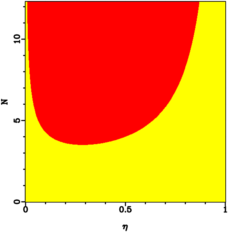
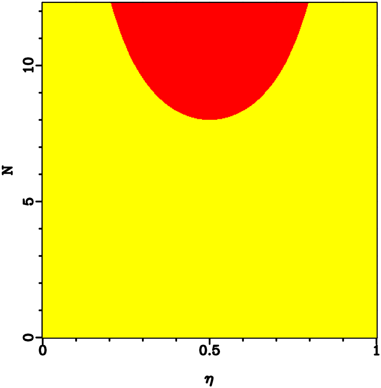
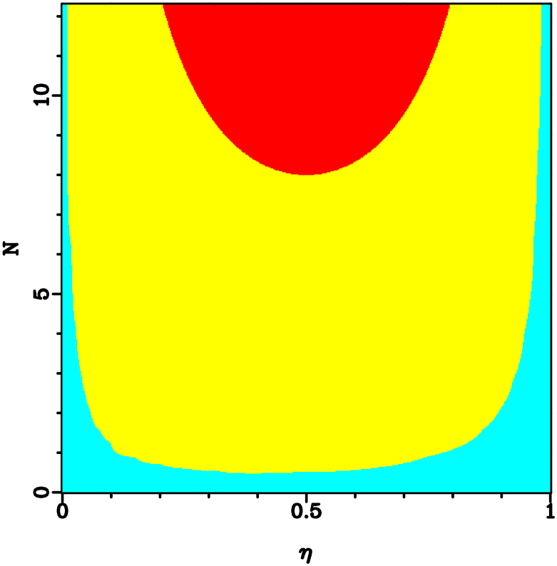
The optimal number of squeezing photons is given by , and it is plotted versus in Fig. 1 for some values of the attenuation . One can see that the optimal fraction of squeezing photons rapidly decreases with attenuation. This means that for increasing loss it is more and more unprofitable to use much power to squeeze the quadrature of the signal, since the quantum noise of the state at the receiver approaches to that of the coherent state. These results agree with previous investigations on the loss effects in terms of signal-to-noise ratio[4]. Figs. 2 and 3 are optimality capacity diagrams, which compare different channels giving the regions on the loss-power plane where each channel is optimal. The coherent-state channel is compared to the squeezed-state channel without and with loss-dependent optimization in Fig. 2 and Fig. 3, respectively. One can see that the optimization leads to a sizeable improvement of the mutual information, especially for strong attenuation and low power (see also Fig. 4), making the diagram symmetric around the vertical axis. Notice the location of the minimum at and on the boundary between the optimality regions in Fig. 3: this means that for mean power less than eight photons the squeezed-state channel always beats the coherent-state one, independently on attenuation.
Through a kind of exclusion principle for the information contents of quantum observables [6], Hall has proved an upper bound for the information that can be achieved by a homodyne channel subjected to Gaussian noise. Following Hall’s method, here we prove the following upper bound for any lossy channel that uses homodyne detection
| (33) |
By denoting with the entropy associated to the probability distribution of the eigenvalue of the observable when the state is , namely
| (34) |
the mutual information retrieved from the measurement of the observable on a member of the ensemble specified by the density matrix is given by
| (35) |
A simple variational calculation gives the upper bounds
| (36) | |||
| (37) |
for the entropy associated to the conjugated quadratures and , the notation representing the ensemble average with density operator .
Moreover, writing as a mixture of pure states
| (38) |
from the concavity of entropy one has
| (39) |
and analogously for the other quadrature . A derivation similar to that of Eq. (28) leads to the conditional probability
| (40) | |||||
| (41) |
where we introduced the Gaussian operator-valued measure defined as follows
| (42) |
By varying over the bra the following quantity
| (43) |
one obtains the variational equation
| (44) | |||
| (45) |
where is the Lagrange multiplier for the normalization constraint relative to the state . It can be easily verified that the case of vacuum state satisfies Eq. (45). Then, from Eq. (39) along with the following relation
| (46) |
that holds for any quadrature operator , one has
| (47) |
On the other hand, from Eqs. (36) and (37) one obtains
| (48) |
The product of the expectation values in Eq. (48) can be maximized as follows
| (49) | |||
| (50) |
and we obtain
| (51) |
Finally, inequalities (47) and (51), together with Eq. (35) yield the information exclusion relation
| (52) |
where . From Eq. (52) the bound (33) follows as a particular case. From the above derivation we see that the bound (33) holds for any lossy channel that employs homodyne detection.
The upper bound (33) is trivially achieved for by a Gaussian ensemble of squeezed states, however, in the presence of loss it is not reached by our optimized channel. As a matter of fact, there is still room for a slight improvement of the mutual information if one allows the squeezing to vary as a function of the signal in Eq. (18). However, such further optimization is not achievable analytically—due to the now non Gaussian form of the conditional probability density—nor it can be worked out numerically, as no viable method is at hand.
IV Direct-detected channel
The ideal communication channel that uses direct detection of Fock-states with thermal a priori probability
| (53) |
achieves the ultimate quantum capacity (the Holevo’s bound [1, 2]) with the constraint of fixed average number of photons . The ultimate quantum capacity is given by
| (54) |
For ideal transmission the conditional probability density is given by the Kronecker delta . In the presence of loss this is replaced by the binomial distribution
| (55) |
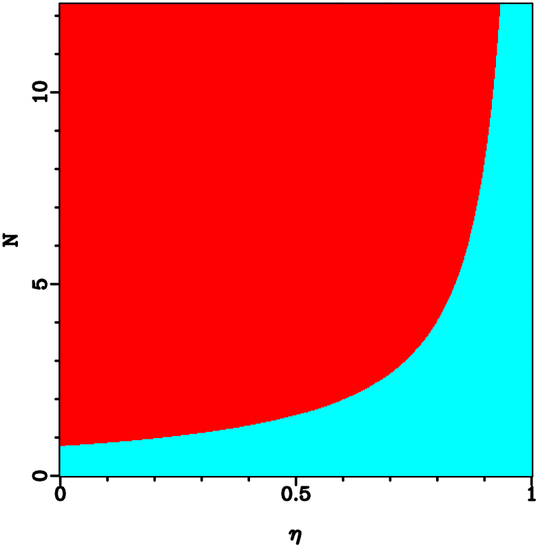
which represents the probability of detecting photons when the transmitted state is . The number-state channel is more sensitive to loss than the coherent-state and the squeezed-state ones. In Fig. 5 the mutual information for the three channels is plotted versus , at fixed power , and with the customary a priori probabilities optimized for the lossless case [Eqs. (17), (22) and (53)]. One can see that at this power level a signal attenuation of 0.5 dB is sufficient to degrade the number-state channel below the capacity of the coherent-state channel, whereas at higher power levels the effect is even more dramatic. The optimality capacity diagram in Fig. 6 compares the number-state with the coherent-state channels. One can see that in the presence of loss the number-state channel rapidly loses off its efficiency, especially for high power and strong attenuation.
Now we address the problem of optimizing the a priori probability distribution in the presence of loss. In principle one could perform the optimization analytically by varying the information over the infinite set of variables , however with no viable method for constraining each to be nonnegative. For this reason we decided to carry out the optimization numerically, using the recursive Blahut’s algorithm[7]. The recursion is given by
| (56) | |||||
| (57) |
where is the a priori probability at the th iteration, is the conditional probability (55), and is the Lagrange multiplier for the average-power constraint. The series are actually truncated to a finite dimension, corresponding to a maximum allowed number of photons. Blahut proved that the quantity
| (58) |
is increasing versus , and achieves the desired bound, and denoting the mutual information and the average photon number with the th iterated a priori probability . For a given one evaluates the limit of for under the recursion (57), and determines the mutual information and the mean photon number for such limiting : in this way the capacity versus power is obtained as parameterized by .
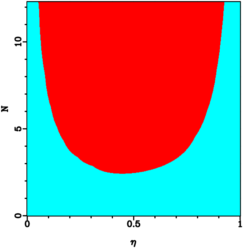
Now we present some numerical results. Figs. 7 show the number probability distribution for different values of loss and power, evaluated by means of the Blahut’s recursive algorithm, stopped at iterations. The Hilbert space has been truncated at dimension 200, however, truncation at 100 gives almost identical results. For stronger loss, the optimal a priori probability departs from the thermal-like behavior, with an enhanced vacuum probability. For loss (see Fig. 7) the probability plot develops gaps of zero probability at intermediate numbers of photons. This can be intuitively understood as the effect of a loss so strong that it becomes more convenient to use a smaller alphabet of well-spaced letters in order to achieve a better distinguishability at the receiver. The increase of the probability pertinent the vacuum state comes clearly from the constant-energy constraint. Table I provides a list of numerical results pertaining Figs. (7). It gives the per cent improvement of the mutual information after optimization, along with the absolute value of the mutual information for the optimized number-state channel, for the number-state channel with customary thermal probability and for the coherent-state channel at given value of the loss and of the mean photon number. Also the values of the quantities and are reported, for convergence estimation of the Blahut’s recursion (58). They are defined as the increment of the quantity in Eq. (58), and the distance between probability plots, both and being evaluated at the last iteration step . One can see that, according to the small values of and , the algorithm is converging quite fast (indeed only 10 steps are usually sufficient to get an estimate of the capacity up to the second digit). With the occurrence of gaps in the a priori probability, the relative improvement of the mutual information increases even more dramatically, up to for strong attenuation . At low power, this improvement allows the direct-detection channel to overcome the coherent-state channel capacity [see Figs. 7a,c,e,g,h and their pertaining numerical values in Table I]. The optimality capacity diagram in Fig. 8 compares the optimized number-state channel with the coherent-state channel. Notice the difference with respect to Fig. 3: here the optimized number-state channel beats the heterodyne channel at power much lower than for the optimized squeezed-state channel in Fig. 3. As for the squeezed-state channel, the optimization makes the diagram more symmetric around the vertical axis.
V Conclusions
We analyzed the detrimental effect of loss on narrow-band quantum-optical channels based on heterodyne detection of coherent states, homodyne detection of squeezed states and direct detection of number states. We have shown that the squeezed-state channel and, even more, the number-state channel, are both easily degraded by loss below the capacity of the coherent-state channel. Because of the peculiar form of the master equation for the loss, the coherent-state channel does not need optimization, and remains as the most efficient one at sufficiently high power.
The optimization of the squeezed-state channel leads to a sizeable improvement of the mutual information (over 30% for at low power). Correspondingly, the optimal fraction of squeezing photons rapidly decreases with attenuation. For total average number of photons the squeezed-state channel is always more efficient than the coherent-state one, independently on attenuation . The optimization has been performed at constant squeezing, whereas the problem of optimizing a signal-dependent squeezing is still open.
As regards the number-state channel, we applied the Blahut’s recursive algorithm to evaluate the optimal a priori probability and the channel capacity. The improvement of the mutual information is considerable, achieving for . The optimal a priori probability departs from the usual monotonic thermal-like distribution, and for it develops gaps of zero probability at intermediate number of photons. At low power the optimization of the number-state channel makes its capacity better than that of the coherent-state channel.
A comprehensive view of the numerical results of this paper is offered by the optimality capacity diagram in Fig. 9: there one can find the regions on the loss-power plane where the coherent-state, the optimized squeezed-state, and the optimized number-state channels are respectively optimal.
Acknowledgments
We gratefully acknowledge interesting and stimulating discussions with H. P. Yuen, who also attracted our attention on the main issue of this paper.


| plot | % | |||||||
|---|---|---|---|---|---|---|---|---|
| a) | .9 | 8.575 | 3.157 | 3.097 | 3.124 | 1.93 | 2 | 1 |
| b) | .75 | 2.827 | 1.775 | 1.699 | 1.642 | 4.50 | 4 | 1 |
| c) | .6 | 2.414 | 1.340 | 1.218 | 1.292 | 10.03 | 1 | 1 |
| d) | .6 | 6.930 | 1.935 | 1.745 | 2.367 | 10.90 | 2 | 6 |
| e) | .55 | 2.288 | 1.219 | 1.083 | 1.175 | 12.56 | 8 | 7 |
| f) | .55 | 6.729 | 1.803 | 1.595 | 2.233 | 13.07 | 1 | 2 |
| g) | .4 | 1.888 | 0.887 | 0.715 | 0.812 | 24.18 | 6 | 2 |
| h) | .15 | 4.040 | 0.720 | 0.416 | 0.684 | 73.08 | 8 | 2 |
REFERENCES
- [1] A. S. Holevo, Probl. Inf. Trans. 9, 177 (1973).
- [2] H. P. Yuen and M. Ozawa, Phys. Rev. Lett. 70, 363 (1993).
- [3] C. M. Caves and P. D. Drummond, Rev. Mod. Phys. 66, 481 (1994), and references therein.
- [4] K. Yamazaki, O. Hirota and M. Nakagawa, Trans. IEICE, E71, 8, 775 (1988).
- [5] M. J. W. Hall, Phys. Rev. A 50, 3295 (1994).
- [6] M. J. W. Hall, Phys. Rev. Lett. 74, 3307 (1995).
- [7] R. E. Blahut, IEEE Trans. Inform. Theory, IT-18, 460 (1972).
- [8] R. G. Gallagher, Information Theory and Reliable Communication (Wiley, New York, 1968).
- [9] G. Lindblad, Commun. Math. Phys. 48, 119 (1976).