A Quantum-Theoretic Analog for a Pair of Noncommuting Observables of the Semiclassical Brillouin Function

Abstract

We study, with the use of numerical integration, a noncommutative extension of a quantum-theoretic model (an alternative to the semiclassical Brillouin function) — recently presented by Brody and Hughston and, independently, Slater — for the thermodynamic behavior of a spin-${1\over 2}$ particle. Differences between the (broadly similar) predictions yielded by this extended model and those obtained from its conventional (semiclassical/Jaynesian) entropy-maximization counterpart are examined.

The Brillouin function,

$$-E=\tanh{\beta},$$ (1)

where $E$ is the expected energy and $\beta$, the inverse temperature parameter, has long served as a model of the thermodynamic behavior of an ensemble of $N$ noninteracting identical spin-${1\over 2}$ particles in an applied magnetic field [1]. In our simplified notation, we take $\beta$ to represent ${\mu B\over kT}$, where $k$ is Boltzmann’s constant, $\mu$ is the particle’s magnetic moment, $B$ is the external field strength, $T$ is the temperature, and $\mu B=h$, where $h$ is Planck’s constant. So, we set $h=1$.

Recently, Brody and Hughston [2] have argued that the theoretical underpinnings of (1) are semiclassical in nature, since the weighting of the phase space volume is eliminated, and random phases are averaged. Park and Band, in an extended series of papers [3], questioned the conceptual foundations of the semiclassical/Jaynesian approach to quantum statistical thermodynamics (cf. [4]) — from which (1) can be derived [5, p. 187]. Balian and Balasz [6] did, however, provide a rigorous justification (making use of field-theoretic concepts) for the Jaynesian (maximum-entropy) method, but, let us note that their argument was asymptotic in nature, relying upon a “supersystem” consisting of $N$ replicas of the system, for which they required that $N\rightarrow\infty$.

Based on certain metrical considerations, Brody and Hughston proposed as a quantum-theoretic alternative to (1), the function,

$$-E={I_{2}(\beta)\over I_{1}(\beta)},$$ (2)

where the $I$’s represent modified (hyperbolic) Bessel functions. (This result was also presented — in a graphical manner — in a somewhat earlier paper of Slater [7].) Bessel functions often appear in the distribution of spherical and directional random variables [8]. Ratios of modified Bessel functions, such as occur in (2), play “an important role in Bayesian analysis” [8]. It seems important to note, in this regard, the identity,

$$\tanh{\beta}={I_{{1\over 2}}(\beta)\over I_{-{1\over 2}}(\beta)}.$$ (3)

Lavenda [9, pp. 193 and 198] has argued, at considerable length, that the Brillouin function (1) lacks a suitable probabilistic basis, because the integral form for the modified Bessel function $I_{\nu}$ exists only for $\nu>{1\over 2}$.

The relation (3) has been used in expressing the expected energy of the linear-chain-lattice case ($d=1$) of the $D$-vector (or $n$-vector) model for $D=1$ [10, p. 492], [11, p. 370], while the relation (2) emerges for the instance $D=4$. The general expression in question takes the form,

$$-E={I_{{D\over 2}}(\beta)\over I_{{D\over 2}-1}(\beta)}.$$ (4)

The reason that the specific dimension four, thus, arises in interpreting the analyses of Brody and Hughston [2] and Slater [7], would appear to be due to the fact that the spin-${1\over 2}$ states (both mixed and pure) can be considered to lie on the surface of a hemisphere in four-dimensional Euclidean space, equipped with the (natural) Bures or statistical distinguishability metric [12, 13, 14]. Let us also observe that the (classical) Langevin function [1] too is expressible as a ratio of modified Bessel functions, that is ($D=3$),

$$\coth{\beta}-{1\over\beta}={I_{{3\over 2}}(\beta)\over I_{{1\over 2}}(\beta)}.$$ (5)

We also point out that the analysis in [7] leads to the result (cf. (2)) corresponding to $D=6$,

$$-E={I_{3}(\beta)\over I_{2}(\beta)},$$ (6)

for the five-dimensional convex set (the unit ball in five-space) of quaternionic two-level systems [15]. (The result (2) is based on the three-dimensional convex set — the “Bloch sphere”, that is, the unit ball in three-space — of the standard complex two-level systems, which, as just mentioned above, also can be viewed as forming a hemisphere in four-space [12].)

Brody and Hughston have argued that the differences (Fig. 1) in predictions between (1) and (2) might be tested in small systems (that is, small $N$), where “there seems to be no a priori reason for adopting the conventional mixed state approach.”

FIG. 1.: The Brillouin function (1) and the (more steeply-sloped at $\beta=0$) quantum-theoretic alternative (2). The difference between the two curves is of the greatest magnitude (.561292) at $\beta=\pm 1.45489$.

For an extended discussion of the role of negative temperatures, in this context, cf. [11, sec. 3.52].

Brody and Hughston noted that the model (2) yielded a nonvanishing heat capacity at zero temperature. “Since it is known in the case of many bulk substances that the heat capacity vanishes as zero temperature is approached, it would be interesting to enquire if a single electron possesses a different behaviour, as indicated by our results” [2]. They also observed that the increase in magnetization, when the temperature decreases, is slower for their quantum-theoretic result than for the semiclassical one.

In this letter, we extend the specific line of reasoning employed by Slater [7] — based upon the Bures metric [14, 16, 17] — to the case in which, rather than the expectation value ($E$) of one observable (as in [2, 7]), one is interested in fitting the expectation values of two noncommuting observables (cf. [6, 18]). We take these observables,

$$\sigma_{1}={1\over 2}\pmatrix{0&1\cr 1&0\cr},\qquad\sigma_{2}={1\over 2}\pmatrix{0&-i\cr i&0\cr},$$ (7)

to be two of the Pauli matrices. (One might also possibly use, $S_{1}=\sigma_{1}/2,S_{2}=\sigma_{2}/2$, as the spin observables [19, p. 38].) To obtain the conventional (semiclassical/Jaynesian) solution to this problem [20, 21], we express the target density matrix ($\rho$) as

$$\rho=\mbox{exp}{(\Omega\cdot I-\lambda_{1}\sigma_{1}-\lambda_{2}\sigma_{2})},$$ (8)

where $\Omega+1$ and $\lambda_{i}$ are the Lagrange multipliers for the normalization of $\rho$ and the measured value of $\sigma_{i}$, respectively. These multipliers must satisfy

$$\Omega=-\mbox{ln}\mbox{Tr}\exp{(-\lambda_{1}\sigma_{1}-\lambda_{2}\sigma_{2})},$$ (9)

and

$${\partial\Omega\over\partial\lambda_{i}}=\langle\sigma_{i}\rangle.\qquad(i=1,2)$$ (10)

The enforcement of these constraints leads to the result,

$$-\langle\sigma_{i}\rangle={\lambda_{i}\tanh{\sqrt{\lambda_{1}^{2}+\lambda_{2}^{2}}}\over\sqrt{\lambda_{1}^{2}+\lambda_{2}^{2}}}.\qquad(i=1,2)$$ (11)

Setting either $\lambda_{1}=0$ or $\lambda_{2}=0$, we essentially recover the Brillouin function (1).

Now, the volume element of the Bures metric over the three-dimensional convex set (“Bloch sphere”) of spin-${1\over 2}$ systems is [22, eq. (6)] (cf. [23, 24]),

$${1\over 8\sqrt{1-{\langle\sigma_{1}\rangle}^{2}-{\langle\sigma_{2}\rangle}^{2}-{\langle\sigma_{3}\rangle}^{2}}},$$ (12)

where

$$\sigma_{3}={1\over 2}\pmatrix{1&0\cr 0&-1\cr},$$ (13)

is the additional Pauli matrix. If we integrate the term (12) over one of the three coordinates (say, $\langle\sigma_{3}\rangle$), we obtain simply a uniform distribution ($\pi/8$) over the unit disk ($0\leq{\langle\sigma_{1}\rangle}^{2}+{\langle\sigma_{2}\rangle}^{2}\leq 1$). Interpreting this uniform distribution as a density-of-states or structure function, we can apply a bivariate Boltzmann factor, $e^{-\beta_{1}\langle\sigma_{1}\rangle-\beta_{2}\langle\sigma_{2}\rangle}$, to it. Integrating this product over the $\langle\sigma_{2}\rangle$-coordinate (between the limits of $\pm\sqrt{1-{\langle\sigma_{1}\rangle}^{2}}$), we obtain,

$${e^{-\beta_{1}\langle\sigma_{1}\rangle}\pi\sinh{(\beta_{2}\sqrt{1-{\langle\sigma_{1}\rangle}^{2}})}\over 4\beta_{2}}.$$ (14)

The corresponding partition function is the integral of (14) over the remaining coordinate ($\langle\sigma_{1}\rangle$) from -1 to 1. This integration has to be performed numerically. Carrying this out, we are then able, again employing numerical integration, to obtain the (twofold) expected value ($\langle\langle\sigma_{1}\rangle\rangle$) of $\langle\sigma_{1}\rangle$ (Fig. 2) as a function of $\beta_{1}$ and $\beta_{2}$, as well as the variance about this expected value (Fig. 5), and the covariance between $\langle\sigma_{1}\rangle$ and $\langle\sigma_{2}\rangle$ (Fig. 8). (The covariance is the expected value — with respect to the Boltzmann distribution — of the product $(\langle\sigma_{1}\rangle-\langle\langle\sigma_{1}\rangle\rangle)(\langle\sigma_{2}\rangle-\langle\langle\sigma_{2}\rangle\rangle)$.)

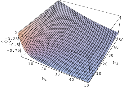
FIG. 2.: The expected value of the expected value of the observable $\sigma_{1}$ as a function of the inverse temperature parameters, $\beta_{1}$ and $\beta_{2}$, of the quantum-theoretic model

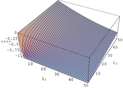
FIG. 3.: The expected value of the expected value of the observable $\sigma_{1}$ as a function of the inverse temperature parameters, $\lambda_{1}$ and $\lambda_{2}$, of the semiclassical (Brillouin-type) model

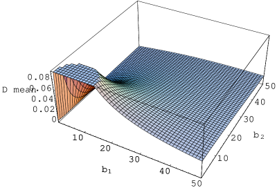
FIG. 4.: The difference between the quantum-theoretic results (Fig. 2) and the semiclassical ones (Fig. 3) for the expected value of the expected value of the observable $\sigma_{1}$ — having identified the $\lambda$’s with the corresponding $\beta$’s

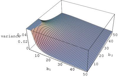
FIG. 5.: The variance of the expected value of the observable $\sigma_{1}$ as a function of the inverse temperature parameters, $\beta_{1}$ and $\beta_{2}$, of the quantum-theoretic model

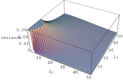
FIG. 6.: The variance of the expected value of the observable $\sigma_{1}$ as a function of the inverse temperature parameters, $\lambda_{1}$ and $\lambda_{2}$, of the semiclassical (Brillouin-type) model

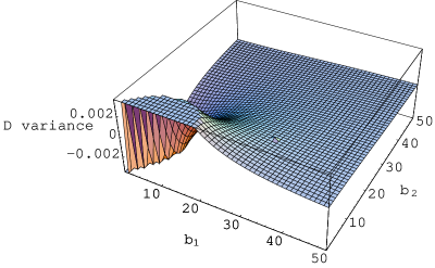
FIG. 7.: The difference between the quantum-theoretic results (Fig. 5) and the semiclassical ones (Fig. 6) for the variance of the expected value of the observable $\sigma_{1}$ — having identified the $\lambda$’s with the corresponding $\beta$’s

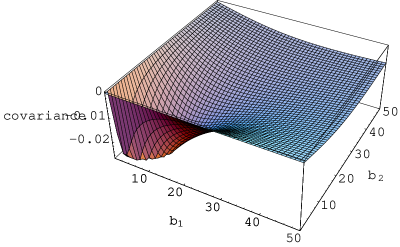
FIG. 8.: The covariance between the expected values of the observables $\sigma_{1}$ and $\sigma_{2}$ as a function of the inverse temperature parameters, $\beta_{1}$ and $\beta_{2}$, of the quantum-theoretic model

FIG. 9.: The covariance between the expected values of the observables $\sigma_{1}$ and $\sigma_{2}$ as a function of the inverse temperature parameters, $\lambda_{1}$ and $\lambda_{2}$, of the semiclassical (Brillouin-type) model

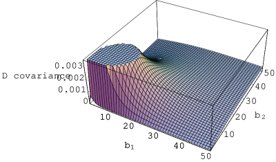
FIG. 10.: The difference between the quantum-theoretic results (Fig. 8) and the semiclassical ones (Fig. 9) for the covariance of the expected values of the observables $\sigma_{1}$ and $\sigma_{2}$— having identified the $\lambda$’s with the corresponding $\beta$’s

For comparison purposes (cf. Fig. 1), we present the semiclassical (noncommuting Brillouin) counterparts to these quantum-theoretic results in the companion figures (Figs. 3, 6, 9). We note strong qualitative resemblances between the two members of each of these three pairs of figures. We also present in Figs. 4, 7 and 10, the differences obtained (after setting $\lambda_{i}$ to $\beta_{i}$, $(i=1,2)$) by subtracting the semiclassical results (shown in Figs. 3, 6 and 9) from the corresponding quantum-theoretic ones (given in Figs. 2, 5 and 8). The most substantial differences in all three cases appear in the vicinity of the (high-temperature) origin ($\beta_{1}=\beta_{2}=0$).

Let us, in conclusion, consider the possibility of expanding the analyses above to the case of three noncommuting observables, rather than two. Then, we would apply a trivariate Boltzmann factor, $e^{-\beta_{1}\langle\sigma_{1}\rangle-\beta_{2}\langle\sigma_{2}\rangle-\beta_{3}\langle\sigma_{3}\rangle}$, to the volume element (12) itself of the Bures metric (rather than its two-dimensional [uniform] marginal — ${\pi\over 8}$). Integrating out the $\langle\sigma_{3}\rangle$-coordinate (between the limits $\pm\sqrt{1-{\langle\sigma_{1}\rangle}^{2}-{\langle\sigma_{2}\rangle}^{2}}$), we obtain (cf. (14)),

$${\pi e^{-\beta_{1}\langle\sigma_{1}\rangle-\beta_{2}\langle\sigma_{2}\rangle}J_{0}(\beta_{3}\sqrt{{\langle\sigma_{1}\rangle}^{2}+{\langle\sigma_{2}\rangle}^{2}})\over 8},$$ (15)

where $J_{0}$ is a Bessel function of the first kind. To obtain the corresponding partition function, it then appears necessary, similarly to before, to numerically integrate (15) over the unit disk $(0\leq{\langle\sigma_{1}\rangle}^{2}+{\langle\sigma_{2}\rangle}^{2}\leq 1)$.

- [1] J. A. Tusyński and W. Wierzbicki, Amer. J. Phys. 59, 555 (1991).
- [2] D. C. Brody and L. P Hughston, The Quantum Canonical Ensemble, quant-ph/9709048 (23 Sep 1997).
- [3] J. L. Park and W. Band, Found. Phys. 6, 157, 249 (1976); 7, 233, 705 (1977).
- [4] J. L. Park, Found. Phys. 18, 225 (1988).
- [5] J. J. Sakurai, Advanced Quantum Mechanics, (Addison-Wesley, Redwood City, 1985).
- [6] R. Balian and N. L. Balazs, Ann. Phys. (NY) 179, 97 (1987).
- [7] P. B. Slater, Bayesian Thermostatistical Analyses of Two-Level Complex and Quaternionic Quantum Systems, quant-ph/9710057 (24 Oct 1997). This paper was submitted (in a non-TeX form) for publication in Dec. 1995, but not accepted. In light of the Brody/Hughston paper [2], the author transcribed it into TeX and placed it in the Los Alamos archive, as well as asked for a reconsideration (which has been granted) of his original submission.
- [8] C. Robert, Stat. Prob. Lett. 9, 155 (1990).
- [9] B. H. Lavenda, Thermodynamics of Extremes. (Albion, West Sussex, 1995).
- [10] H. E. Stanley, in Phase Transitions and Critical Phenomena: Series Expansions for Lattice Models, edited by C. Domb and M. S. Green (Academic, New York, 1974), vol. 3.
- [11] H. S. Robertson, Statistical Thermophysics, (Prentice-Hall, Englewood Cliffs, 1993).
- [12] S. L. Braunstein and G. J. Milburn, Phys. Rev. A 51, 1820 (1995).
- [13] A. Uhlmann, J. Geom. Phys. 18, 76 (1996).
- [14] M. Hübner, Phys. Lett. A 163, 239 (1992).
- [15] S. L. Adler, Quaternionic Quantum Mechanics and Quantum Fields, (Oxford, New York, 1995).
- [16] M. Hübner, Phys. Lett. A 179, 226 (1993).
- [17] S. L. Braunstein and C. M. Caves, Phys. Rev. Lett. 72, 3439 (1994).
- [18] H. Haken, Information and Self-Organization: A Macroscopic Approach to Complex Systems, (Springer-Verlag, Berlin, 1988).
- [19] L. C. Biedenharn and J. D. Louck, Angular Momentum in Quantum Physics, (Addison-Wesley, Reading, 1981).
- [20] E. T. Jaynes, Phys. Rev. 108, 171 (1957).
- [21] P. R. Dukes and E. G. Larson, in Maximum Entropy and Bayesian Methods, edited by W. T. Grandy Jr. and L. H. Schick (Kluwer, Dordrecht, 1991), pp. 161-168.
- [22] P. B. Slater, J. Phys. A, L271 (1996).
- [23] P. B. Slater, J. Math. Phys. 37, 2682 (1996).
- [24] P. B. Slater, J. Math. Phys. 38, 2274 (1997).