On (non)linear Quantum Mechanics

Abstract

We review a possible framework for (non)linear quantum theories, into which linear quantum mechanics fits as well, and discuss the notion of “equivalence” in this setting. Finally, we draw the attention to persisting severe problems of nonlinear quantum theories.

I Nonlinearity in quantum mechanics

Nonlinearity can enter quantum mechanics in various ways, so there are a number of associations a physicist can have with the term “nonlinear quantum mechanics”. Because of this, we shall start with a (certainly incomplete) list of those ways that we shall not deal with here.

In quantum field theory nonlinearity occurs in the equations of interacting field operators. These equations may be quantizations of nonlinear classical field equations (see e.g. [1]) or mathematically tractable models as in $\phi^{4}$-theory. Here, however, the field operators remain linear, as does the whole quantum mechanical setup for these quantum field theories.

On a first quantized level, nonlinear terms have been proposed very early for a phenomenological and semi-classical description of self-interactions, e.g. of electrons in their own electromagnetic field (see e.g. [2]). Being phenomenological these approaches are build on linear quantum mechanics and use the standard notion of observables and states. For complex systems the linear multi-particle Schrödinger equation is often replaced by a nonlinear single-particle Schrödinger equation as in the density functional theory of solid state physics.

There have also been attempts to incorporate friction on a microscopic level using nonlinear Schrödinger equations. Many of these approaches incorporate stochastic frictional forces in the nonlinear evolution equation for the wavefunctions (see e.g. [3]).

Contrary to these, we are concerned with a more fundamental role of nonlinearity in quantum mechanics. Notable efforts in this direction have been launched, for example, by Bialinycki-Birula and Mycielski [4], Weinberg [5], and Doebner and Goldin [6, 7].

II Problems of a fundamentally nonlinear nature

There are evident problems, if we merely replace (naively) the evolution equation of quantum mechanics, i.e. the linear Schrödinger equation, by a nonlinear variant, but stick to the usual definitions of linear quantum mechanics, like observables being represented by self-adjoint operators, and states being represented by density matrices.

Density matrices ${\mathbf{W}}\in{\mathcal{T}}_{1}^{+}({\mathcal{H}})$ represent in general a couple of different, but indistinguishable mixtures of pure states,

$$\sum_{j}\lambda_{j}|\psi_{j}\rangle\langle\psi_{j}|={\mathbf{W}}=\sum_{j}\lambda_{j}^{\prime}|\psi_{j}^{\prime}\rangle\langle\psi_{j}^{\prime}|\,,\\$$ (1)

where $\{(\lambda_{j},\psi_{j})\}_{j=1,\ldots}$ and $\{(\lambda_{j}^{\prime},\psi_{j}^{\prime})\}_{j=1,\ldots}$ are different mixtures of pure states $\psi_{j}$ and $\psi_{j}^{\prime}$ with weights $\sum_{j}\lambda_{j}=1$ and $\sum_{j}\lambda_{j}^{\prime}=1$, respectively. This identification of different mixtures is evidently not invariant under a nonlinear time-evolution $\Phi_{t}$ of the wavefunctions,

$$\sum_{j}\lambda_{j}|\Phi_{t}(\psi_{j})\rangle\langle\Phi_{t}(\psi_{j})|\stackrel{{\scriptstyle i.g.}}{{\neq}}\sum_{j}\lambda_{j}^{\prime}|\Phi_{t}(\psi_{j}^{\prime})\rangle\langle\Phi_{t}(\psi_{j}^{\prime})|\\$$ (2)

This apparent contradiction has been used by Gisin, Polchinski, and others [8, 9] to predict superluminal communications in an EPR-like experiment for any nonlinear quantum theory.

Rather than taking this observation as an inconsistency of a nonlinear quantum theory (e.g. as in [10, 11]), we take it as an indication, that the notions of observables and states in a nonlinear quantum theory have to be adopted appropriately [12]. If nonlinear quantum mechanics is to remain a statistical theory, we need a consistent and complete statistical interpretation of the wave function and the observables, and therefore a consistent description of mixed states.

III Generalized quantum mechanics

In view of the intensive studies on nonlinear Schrödinger equations in the last decade it is astonishing to note that a framework for a consistent framework of nonlinear quantum theories has already been given by Mielnik in 1974 [13]. We shall adopt this approach here and develop the main ingredients of a quantum theory with nonlinear time evolutions of wavefunctions.

Our considerations will be based on a fundamental hypothesis on physical experiments:

All measurements can in principle be reduced to a change of the dynamics of the system (e.g. by invoking external fields) and positional measurements.

In fact, this point of view, which has been taken by a number of theoretical physicists [13, 14, 15, 16], becomes most evident in scattering experiments, where the localization of particles is detected (asymptotically) after interaction.

Based on this hypothesis we build our framework for a nonlinear quantum theory on three main “ingredients” [17]:

First, a topological space${\mathcal{T}}$ of wavefunctions. In the one particle examples below, this topological space is a Hilbert space of square integrable functions, but we may also think of other function spaces [18].

Secondly, the time evolutions are given by homeomorphisms of ${\mathcal{T}}$,

$$\Phi_{t}^{(Ext)}\colon\,{\mathcal{T}}\to{\mathcal{T}}\,,$$ (3)

which depend on the time interval $t$ and the external conditions (e.g. external fields) $Ext\in{\mathcal{C}}$. Mielnik’s motion group ${\mathcal{M}}$ [13] is the smallest (semi-) group containing all time evolutions $\Phi_{t}^{(Ext)}$, close in the topology of pointwise convergence.

Finally, positional observables ${\mathcal{P}}$ are represented by probability measures on physical space $M$, which depend on the wavefunction $\phi\in{\mathcal{T}}$, i.e. ${\mathcal{P}}=\bigl{\{}p_{B}\bigm{|}B\in{\mathcal{B}}(M)\bigr{\}}$, where

$$p_{B}:{\mathcal{T}}\to[0,1]\,,\qquad\sum_{k=1}^{\infty}p_{B_{k}}=p_{B}\,,\quad B=\bigcup_{k=1}^{\infty}B_{k},$$ (4)

for disjoint $B_{k}\in{\mathcal{B}}(M)$.

We shall call the triple $({\mathcal{T}},{\mathcal{M}},{\mathcal{P}})$ a quantum system. Using these basic ingredients we can define effects and states of the quantum system $({\mathcal{T}},{\mathcal{M}},{\mathcal{P}})$ as derived concepts. An effect (or a counter) is (at least approximately in the sense of pointwise convergence) a combination of evolutions $T\in{\mathcal{M}}$ and positional measurements $p\in{\mathcal{P}}$, i.e.

$${\mathcal{E}}:=\overline{\left\{p\circ T\left|p\in{\mathcal{P}},T\in{\mathcal{M}}\right\}\right.}^{p.c.}$$ (5)

is the set of effects. A general observable $A$ is an ${\mathcal{E}}$-valued measure on the set $M^{A}$ of its classical values,

$$p^{A}\colon\,{\mathcal{B}}(M^{\!A})\to{\mathcal{E}}\,,\quad p^{A}_{M^{\!A}}[\phi]=1\,.$$ (6)

The standard example of such an asymptotic observable is the (dynamical) momentum of a single particle of mass $m$ in $\bf R^{3}$. Let $B\in{\mathcal{B}}(\bf R^{3}_{p})$ be an open subset of momentum space $\bf R_{p}^{3}$, then

$$B_{t}:=\Bigl{\{}\frac{t}{m}\vec{p}\,\Bigm{|}\,\vec{p}\in B\Bigr{\}}\,,$$ (7)

defines the corresponding velocity cone, see Figure 1.

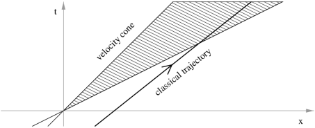
FIG. 1.: Velocity cone for the asymptotic measurement of momentum.

If $\Phi_{t}^{(0)}$ denotes the free quantum mechanical time evolution of our theory — provided, of course, there is such a distinguished evolution — the limit

$$p^{P}_{B}[\phi]:=\lim_{t\to\infty}p_{B_{t}}\Bigl{[}\Phi_{t}^{(0)}[\phi]\Bigr{]}$$ (8)

defines a probability measure on $\bf R^{3}_{p}$, so that the momentum observable is given by the ${\mathcal{E}}$-valued measure

$$P=\Bigl{\{}p^{P}_{B}\in{\mathcal{E}}\Bigm{|}B\in{\mathcal{B}}(\bf R^{3}_{p})\Bigr{\}}\,.$$ (9)

Coming back to the general framework, once we have determined the set of effects, we can define the states of the quantum system as equivalence classes of mixtures of wavefunctions.

Different mixtures of wave functions

$$\pi=\bigl{\{}(\lambda_{j},\phi_{j})\bigr{\}}_{j=1,\ldots}\,,\quad\sum_{j}\lambda_{j}=1\,,$$ (10)

with corresponding effects $f[\pi]:=\sum_{j}\lambda_{j}f(\phi_{j})$ may be indistinguishable with respect to the effects ${\mathcal{E}}$,

$$\pi_{1}\sim\pi_{2}\quad\Leftrightarrow\quad\Bigl{(}f[\pi_{1}]=f[\pi_{2}]\quad\forall\,f\in{\mathcal{E}}\Bigr{)}\,.$$ (11)

Hence, the state space

$$\SS:=\raisebox{5.0pt}{$\displaystyle\Pi({\mathcal{T}})$}\kern-3.00003pt/\kern-1.00006pt\raisebox{-5.0pt}{$\displaystyle\sim$}$$ (12)

is a convex set with pure states as extremal points ${\mathcal{E}}(\SS)$.

IV Linear quantum mechanics

Generalized quantum mechanics is indeed a generalization of linear quantum mechanics, as the latter is contained in the general framework as a special case. To see this, we consider a non-relativistic particle of mass $m$ in $\bf R^{3}$ (Schrödinger particle), defined in our setting as a quantum system $({\mathcal{H}},{\mathcal{M}}_{S},{\mathcal{P}}_{\chi})$ with the topological space of wave functions as the Hilbert-space

$${\mathcal{T}}\equiv{\mathcal{H}}\equiv L^{2}(\bf R^{3},d^{3}x)\,,$$ (13)

the Born interpretation of $\kern 1.00006pt^{|\psi(\vec{x})|^{2}}\kern-3.00003pt/\kern-1.00006pt_{\|\psi\|^{2}}$ as a positional probability density on $\bf R^{3}$, i.e.

$$p_{B}[\psi]:=\frac{\langle\psi|{\mathbf{E}}(B)\psi\rangle}{\|\psi\|^{2}}=\frac{\|{\mathbf{E}}(B)\psi\|^{2}}{\|\psi\|^{2}}$$ (14)

defines the positional observables, and unitary time evolutions generated by linear Schrödinger equations

$$i\hbar\partial_{t}\psi_{t}=\left(-\frac{\hbar^{2}}{2m}\Delta+V\right)\psi_{t}\equiv{\mathbf{H}}_{V}\psi_{t}\,,$$ (15)

with a class of suitable potentials $V$ representing the external conditions of the system.

Starting with these three objects we recover indeed the full structure of (linear) quantum mechanics. First, the motion group of the Schrödinger particle is the whole unitary group [19]

$${\mathcal{M}}_{S}\simeq U({\mathcal{H}})\,.$$ (16)

Furthermore, the (decision) effects are given precisely by orthogonal projection operators [20],

$${\mathcal{E}}\simeq{\mathit{Proj}}({\mathcal{H}})\,,\quad f_{{\mathbf{E}}}[\psi]=\frac{\|{\mathbf{E}}\psi\|^{2}}{\|\psi\|^{2}}\,,$$ (17)

so that the logical structure of quantum mechanics is recovered; observables occur naturally through their spectral measures in this scheme. For example, the asymptotic definition of momentum along the lines given above is well known in linear quantum mechanics [21] and leads through standard Fourier transform to the usual spectral measure of the momentum operator ${\mathbf{P}}$.

Finally, as a consequence of the above set of effects, the state space coincides with the space of normalized, positive trace class operators,

$$\SS\simeq{\mathcal{T}}_{1}^{+}({\mathcal{H}})\,,\qquad{\mathcal{E}}(\SS)\simeq P({\mathcal{H}})\,.$$ (18)

V Equivalent quantum systems

Having based our discussion on a fundamental hypothesis on the distinguished role of positional measurements in quantum mechanics, the notion of gauge equivalence has to be reconsidered within the generalized framework of the previous section.

As our framework is based on topological spaces, two quantum systems $({\mathcal{T}},{\mathcal{M}},{\mathcal{P}})$ and $(\widehat{\mathcal{T}},\widehat{\mathcal{M}},\widehat{\mathcal{P}})$ are topologically equivalent, if ${\mathcal{P}}$ and $\widehat{\mathcal{P}}$ are positional observables on the same physical space $M$, the time evolutions depend on the same external conditions ${\mathcal{C}}$, and there is a homeomorphism $N\colon\,{\mathcal{T}}\to\widehat{\mathcal{T}}$, such that

$$\begin{array}[]{rcll}p_{B}&=&\widehat{p}_{B}\circ N\,,&\forall B\in{\mathcal{B}}(M)\,,\\ {\Phi}_{t}^{(Ext)}&=&N^{-1}\circ\widehat{\Phi}_{t}^{(Ext)}\circ N\,,&\forall t\in\bf R,\,Ext\in{\mathcal{C}}\,.\end{array}$$ (19)

For the linear quantum systems of the previous section this notion of topological equivalence reduces naturally to ordinary unitary equivalence.

A particular case arises, if we consider automorphisms of the same topological space of wavefunctions ${\mathcal{T}}$ that leave the positional observables invariant,

$$N\colon\,{\mathcal{T}}\to{\mathcal{T}}\,,\qquad p_{B}=p_{B}\circ N\quad\forall B\in{\mathcal{B}}(M)\,.$$ (20)

We call these automorphisms generalized gauge transformations. For linear quantum systems, these reduce to ordinary gauge transformations of the second kind, $\left({\mathbf{U}}_{\theta_{t}}\psi_{t}\right)(\vec{x})=e^{i\theta_{t}(\vec{x})}\psi_{t}(\vec{x})\,.$ As in this linear case, the automorphisms $N$ may be (explicitly) time-dependent.

VI Quantum mechanics in a nonlinear disguise

As we have seen in Section IV, the framework of Section III can in indeed be filled in case of linear evolution equations; but are there also nonlinear models? Mielnik has listed a number of nonlinear toy models for his framework [13] and has furthermore considered finite dimensional nonlinear systems [22]; Haag and Bannier have given an interesting example of a quantum system with linear and nonlinear time evolutions [23].

Here, however, we shall proceed differently in order to obtain nonlinear quantum system: We use the generalized gauge transformations introduced in the previous section in order to construct nonlinear quantum systems $({\mathcal{H}},{\mathcal{M}},{\mathcal{P}})$ with $L^{2}$-wavefunctions that are gauge equivalent to linear quantum mechanics.

To simplify matters, we assume that the time evolution of the nonlinear quantum system is still given by a local, (quasi-)homogeneous nonlinear Schrödinger equation. This leads us to consider strictly local, projective generalized gauge transformations [20]

$$N_{\gamma_{t}}(\psi_{t})=\psi_{t}\exp\left(i\gamma_{t}\ln|\psi_{t}|\right)\,,$$ (21)

where $\gamma_{t}$ is a time-dependent parameter. As these automorphisms of $L^{2}(\bf R^{3},d^{3}x)$ are extremely similar to local linear gauge transformations of the second kind, they have been called nonlinear gauge transformations [24] or gauge transformations of the third kind [25].

Using these transformations, the evolution equations for $\psi_{t}^{\prime}:=N_{\gamma_{t}}(\psi_{t})$, where $\psi_{t}$ is a solution of the linear Schrödinger equation (15) are easily calculated:

$$\begin{array}[]{rcl}\displaystyle i\hbar\partial_{t}\psi_{t}&=&\displaystyle\left(-\frac{\hbar^{2}}{2m}\Delta+V\right)\psi_{t}-i\frac{\hbar^{2}\gamma_{t}}{4m}R_{2}[\psi_{t}]\psi_{t}-\frac{\hbar^{2}\gamma_{t}}{4m}\left(R_{1}[\psi_{t}]-R_{4}[\psi_{t}]\right)\psi_{t}\\ &&\displaystyle+\frac{\hbar^{2}\gamma_{t}^{2}}{16m}\left(2R_{2}[\psi_{t}]-R_{5}[\psi_{t}]\right)\psi_{t}-\frac{1}{2}\dot{\gamma}_{t}\ln|\psi_{t}|^{2}\,\psi_{t}\,,\end{array}$$ (22)

where

$$R_{1}[\psi]:=\frac{\nabla\cdot\vec{J}}{\rho}\,,\quad R_{2}[\psi]:=\frac{\Delta\rho}{\rho}\,,\quad R_{4}[\psi]:=\frac{\vec{J}\cdot\nabla\rho}{\rho^{2}}\,,\quad R_{5}[\psi]:=\frac{\nabla\rho\cdot\nabla\rho}{\rho^{2}}\,.$$ (23)

These equations contain typical functionals $R_{j}$ of the Doebner–Goldin equations [7] as well as the logarithmic term of Bialynicki-Birula–Mycielski [4]. Note that the form of Eq. (22) do not immediately reveal its linearizability, the underlying linear structure of this model is disguised.

In fact, through an iterated process of gauge generalization and gauge closure — similar to the minimal coupling scheme of linear quantum mechanics — we could obtain a unified family of nonlinear Schrödinger equations [25, 26] ($R_{3}[\psi]:=\frac{\vec{J}^{\,2}}{\rho^{2}}$):

$$i\partial_{t}\psi_{t}=i\sum_{j=1}^{2}{\nu_{j}}R_{j}[\psi_{t}]\,\psi_{t}+\mu_{0}V+\sum_{k=1}^{5}{\mu_{k}}R_{k}[\psi_{t}]\,\psi_{t}+{\alpha_{1}}\ln|\psi_{t}|^{2}\,\psi_{t}\,.$$ (24)

VII Final Remarks: Histories and Locality

In this contribution we have sketched a framework for nonlinear quantum theories that generalizes the usual linear one. We close with three remarks.

The first is concerned with the definition of effects (and positional observables) is our framework. Since we have used real-valued measures, our observables do not allow for an idealization of measurements as in the linear theory, where a projection onto certain parts of the spectrum is possible using the projection-valued measure. Combined subsequent measurements (histories) have to be described by quite complicated time evolutions. However, in case of linearizable quantum system, generalized projections

$$E:=N\circ{\mathbf{E}}\circ N^{-1}\,,\qquad{\mathbf{E}}\in{\mathit{Proj}}({\mathcal{H}})$$ (25)

onto nonlinear sub-manifolds of ${\mathcal{H}}$ can be realized as an idealization of measurements, and yield a nonlinear realization of the standard quantum logic [12].

Secondly, we should emphasize that we have not been able to describe a complete and satisfactory nonlinear theory that is not gauge equivalent to linear quantum mechanics. One of the obstacles of quantum mechanical evolution equations like (24) is the difficulty of the (global) Cauchy problem for partial differential equations. Whereas there is a solution for the logarithmic nonlinear Schrödinger equation [27], there are only local solutions for (non-linearizable) Doebner–Goldin equations [28].

Another problem of nonlinear Schrödinger equations in quantum mechanics is the locality of the corresponding quantum theory: EPR-like experiments could indeed lead to superluminal communications, though not in the naive (and irrelevant) fashion described in Section (II), relevant Gisin-effects [29] can occur, if changes of the external conditions in spatially separated regions have instantaneous effects. Since the nonlinear equations we have considered here are separable, this effect can only occur for entangled initial wavefunctions, i.e.

$$V(\vec{x}_{1},\vec{x}_{2})=V_{1}(\vec{x}_{1})+V_{2}(\vec{x}_{2})\,,\qquad\psi_{0}(\vec{x}_{1},\vec{x}_{2})\neq\varphi_{1}(\vec{x}_{1})\varphi_{2}(\vec{x}_{2})\,.$$ (26)

For Doebner-Goldin equations, for instance, such effects indeed occur (at least) for certain subfamilies that are not Galilei invariant [29]; (higher order) calculations for the Galilei invariant case and the logarithmic Schrödinger equation are not yet completed.

In the title of this contribution we have put the prefix “non” in brackets; the remarks above may have indicated why. Finally, one might be forced to find different ways of extending a nonlinear single particle theory to many particles (see e.g. [30, 31]).

Acknowledgments

Thanks are due to H.-D. Doebner, G.A. Goldin, W. Lücke, and R.F. Werner for interesting and fruitful discussions on the subject. I am also greatful to the organizers for their invitation to the “Second International Conference on Symmetry in Nonlinear Mathematical Physics” It is a pleasure to thank Renat Zhdanov, his family and friends for their warm hospitality during our stay in Kiev.

REFERENCES

- [1] Segal, I. E., J. Math. Phys. , 1960, V 1, N 6, 468–479.
- [2] Fermi, E., Atti della Reale Accademia nazionale dei Lincei. Rendiconti., 1927, V 5, N 10, 795–800.
- [3] Messer, J., Lett. Math. Phys. , 1978, V 2, 281–286.
- [4] Bialynicki-Birula, I. and Mycielski, J., Ann. Phys. (NY), 1976, V 100, 62–93.
- [5] Weinberg, S., Phys. Rev. Lett. , 1989, V 62, 485–488.
- [6] Doebner, H.-D. and Goldin, G. A., Phys. Lett. A, 1992, V 162, 397–401.
- [7] Doebner, H.-D. and Goldin, G. A., J. Phys. A: Math. Gen., 1994, V 27, 1771–1780.
- [8] Gisin, N., Phys. Lett. A, 1990, V 143, 1–2.
- [9] Polchinski, J., Phys. Rev. Lett. , 1991, V 66, N 4, 397–400.
- [10] Weinberg, S., Dreams of a Final Thoery, Pantheon Books, New York, 1992.
- [11] Gisin, N., Relevant and irrelevant nonlinear Schr dinger equations, in Doebner et al. [32], 1995 109–124.
- [12] Lücke, W., Nonlinear Schrödinger dynamics and nonlinear observables, in Doebner et al. [32], 1995 140–154.
- [13] Mielnik, B., Comm. Math. Phys. , 1974, V 37, 221–256.
- [14] Feynman, R. and Hibbs, A., Quantum Mechanics and Path Integrals, McGraw-Hill Book Company, New York, 1965.
- [15] Nelson, E., Phys. Rev. , 1966, V 150, 1079–1085.
- [16] Bell, J. S., Rev. Mod. Phys. , 1966, V 38, N 3, 447–452.
- [17] Nattermann, P., Generalized quantum mechanics and nonlinear gauge transformations, in Symmetry in Science IX, editors B. Gruber and M. Ramek. Plenum Press, New York, 1997, 269–280, ASI-TPA/4/97, quant-ph/9703017.
- [18] Nattermann, P., Nonlinear Schrödinger equations via gauge generalization, in Doebner et al. [33], 428–432, ASI-TPA/9/97.
- [19] Waniewski, J., Rep. Math. Phys. , 1977, V 11, N 3, 331–337.
- [20] Nattermann, P., Dynamics in Borel-Quantization: Nonlinear Schrödinger Equations vs. Master Equations, Ph.D. thesis, Technische Universität Clausthal, June 1997.
- [21] Kemble, E. C., The Fundamental Princeiples of Quantum Mechanics with Elementary Applications, Dover Publishing, New York, 1937.
- [22] Mielnik, B., J. Math. Phys. , 1980, V 21, N 1, 44–54.
- [23] Haag, R. and Bannier, U., Comm. Math. Phys. , 1978, V 60, 1–6.
- [24] Doebner, H.-D., Goldin, G. A., and Nattermann, P., A family of nonlinear Schrödinger equations: Linearizing transformations and resulting structure, in Quantization, Coherent States, and Complex Structures, editors J.-P. Antoine, S. Ali, W. Lisiecki, I. Mladenov, and A. Odzijewicz. Plenum Publishing Corporation, New York, 1995, 27–31.
- [25] Doebner, H.-D. and Goldin, G. A., Phys. Rev. A, 1996, V 54, 3764–3771.
- [26] Doebner, H.-D., Goldin, G. A., and Nattermann, P., Gauge transformations in quantum mechanics and the unification of nonlinear Schrödinger equations, ASI-TPA/21/96, quant-ph/9709036, submitted to J. Math. Phys.
- [27] Cazenave, T. and Haraux, A., Ann. Fac. Sc. Toul., 1980, V 11, 21–51.
- [28] Teismann, H., The Cauchy problem for the Doebner–Goldin equation, in Doebner et al. [33], 433–438.
- [29] Lücke, W. and Nattermann, P., Nonlinear quantum mechanics and locality, in Symmetry in Science X, editors B. Gruber and M. Ramek. Plenum Press, New York, 1998, ASI-TPA/12/97, quant-ph/9707055.
- [30] Goldin, G. A., Nonlinear gauge transformations and their physical implications, talk at Symmetry in “Nonlinear Mathematical Physics II”.
- [31] Czachor, M., Complete separability of a class of nonlinear Schrödinger and Liouville-von Neumann equations, quant-ph/9708052.
- [32] Doebner, H.-D., Dobrev, V. K., and Nattermann, P., editors, Nonlinear, Deformed and Irreversible Quantum Systems. World Scientific, Singapore, 1995.
- [33] Doebner, H.-D., Nattermann, P., and Scherer, W., editors, Group21 — Physical Applications and Mathematical Aspects of Geometry, Groups and Algebras, volume 1. World Scientific, Singapore, 1997.