EPR correlations and EPW distributions revisited

Abstract

It is shown that Bell’s proof of violation of local realism in phase space is incorrect. Using Bell’s approach, a violation can be derived also for nonnegative Wigner distributions. The error is found to lie in the use of an unnormalizable Wigner function.

In 1964, J. S. Bell derived an inequality which must be obeyed by any local, realistic theory [1]. Simultaneously, he demonstrated that quantum mechanics violates such an inequality. This was done using a two-particle entangled spin-state. Clauser et al. reformulated Bell’s inequality in a way better adapted to experimental testing [2]. Since then, Bell’s theorem has been extended in many ways [3, 4]. Theoretically, violation of local realism has also been demonstrated without the use of inequalities [5, 6]. Local realism has been tested in various experiments, and in the overwhelming majority of cases a violation has been found [7, 8].

Most of this activity has been concerned with tests where discrete variables are measured. Most typically, entangled spin-$1\over 2$ states [9, 10] are employed. Bell’s paper [1] was inspired by the work of Einstein, Podolsky and Rosen (EPR), which dealt with a gedanken experiment where continuous variables like position and momentum would be observed [11]. In 1985, Horne and Zeilinger proposed a Bell-type experiment using entanglement in continuous variables, in this case linear momenta [12]. This possibility was elaborated further in Refs. [13, 14], and an experimental test was performed by Rarity and Tapster in 1990 [15].

It has been shown that the EPR state can be generated in quantum optics by a nondegenerate parametric amplifier [16, 17]. In this experiment, two conjugate variables can both be observed with arbitrary precision if one of them is inferred from a strongly correlated variable. These predictions were later confirmed in an experiment by Ou et al. [18, 19]. It should be noted that violation of local realism is not demonstrated in such experiments.

In 1986 Bell presented a paper entitled “EPR correlations and EPW distributions” in a conference arranged by the New York Academy of Sciences [20]. It has also been reprinted in the volume “Speakable and unspeakable in quantum mechanics” [21]. In the title, Bell plays with the acronyms EPR and EPW, the latter being formed from the initials of Eugene P. Wigner. The Wigner distribution [22] plays a prominent role in this paper. With a few notable exceptions [23, 24], the paper has received little attention in the litterature. It is different from the other works by Bell on local realism in that it deals with an experiment where variables with a continuous spectrum are to be observed. Bell formulates a condition on local realism for a two-particle system where the particle positions are to be observed at different times. This is closely related to the original EPR problem. The state originally used by EPR has a nonnegative Wigner distribution. Bell argues that this constitutes a local, classical model, and that consequently this state should not violate local realism. He then examines a state with negative Wigner distribution, and proceeds to demonstrate that this state violates local realism.

Recently, Leonhardt and Vaccaro [24] have demonstrated that Bell’s scheme can be translated into a quantum optical experiment. Instead of observing particle positions at different times, they suggested to observe the rotated quadrature variables of a two-mode radiation field at different settings of the local oscillator phases. As the input state, they suggested to use a superposition of vacuum and a two-photon state.

In his 1986 paper [20], Bell used an unnormalizable Wigner function in order to describe a state with sharp momentum. However, the use of vectors with infinite norm may sometimes lead to problems [25]. Due to the infinite norm, Bell could not calculate normalized probabilities. Instead, he introduced an inequality where only relative probabilities enter. With these assumptions he was able to demonstrate violation of local realism. In this paper, I shall follow Bell’s procedure in Ref. [20] closely, but I will use an input state which has an explicitly nonnegative Wigner distribution. Nevertheless, I will derive a violation of Bell’s inequality. This raises the suspicion that there must be something wrong in Bell’s argument in Ref. [20]. And indeed, by closer inspection, it is found that the use of an unnormalizable Wigner function is not permissible, due to the fact that a normalization factor is treated as time independent. This will be explained in detail later.

To begin with, we consider a coherent state $\mid\alpha\rangle$. Here $\alpha=(1/\sqrt{2})(q_{0}+ip_{0})$, and $q_{0}$ and $p_{0}$ are assumed to be real numbers. This state has a Wigner distribution [22, 26]

$$W_{1}(q,p)={1\over\pi}\exp\left[-(q-q_{0})^{2}-(p-p_{0})^{2}\right].$$ (1)

Also, we shall consider a “squeezed vacuum” state, which has a Wigner distribution [26]

$$W_{2}(Q,P)={1\over\pi}\exp\left[-(sQ)^{2}\right]\exp\left[-\left({P\over s}\right)^{2}\right].$$ (2)

When $s$ decreases, the first gaussian gets very broad and almost independent of $Q$, whereas the second gaussian gets very narrow. In the limit $s\rightarrow 0$ Bell writes the Wigner function as

$$W_{2}(Q,P)=K\;\delta(P),$$ (3)

where he denotes $K$ as an “unimportant constant” [20]. Note that in this way he has started working with an unnormalizable Wigner distribution. It is the main purpose of this paper to show that this trick is not permissible.

Assume that the total system is described by the product $W_{1}W_{2}$. Note that both $W_{1}$ and $W_{2}$ are nonnegative. In this sense, a classical phase space description exists. In analogy with Bell’s treatment (see also Bohr in Ref. [27]), we impose the linear transformations

$$q = {1\over\sqrt{2}}(q_{1}-q_{2}),\quad p={1\over\sqrt{2}}(p_{1}-p_{2}),$$ (4)

$$Q = {1\over\sqrt{2}}(q_{1}+q_{2}),\quad P={1\over\sqrt{2}}(p_{1}+p_{2}).$$ (5)

Expressed in terms of output variables, the total Wigner distribution now reads

$$W(q_{1},q_{2},p_{1},p_{2})=W_{1}({q_{1}-q_{2}\over\sqrt{2}},{p_{1}-p_{2}\over\sqrt{2}})W_{2}({q_{1}+q_{2}\over\sqrt{2}},{p_{1}+p_{2}\over\sqrt{2}}).$$ (6)

Now we assume that the two “positions” $q_{1}$ and $q_{2}$ are measured at arbitrary times $t_{1}$ and $t_{2}$, respectively. The times $t_{k}$ play the role of local parameters, just like polarizer settings do in the traditional Bell experiment [1]. For two free particles, the two-time Wigner distribution is [22]

$$W(q_{1},q_{2},p_{1},p_{2},t_{1},t_{2})=W(q_{1}-p_{1}t_{1},q_{2}-p_{2}t_{2},p_{1},p_{2}).$$ (7)

Note that this distribution is also nonnegative. We assume that the two masses are equal, and choose a unit of mass so that $m_{k}=1$. The two-time, marginal, joint position probability distribution is

$$w(q_{1},q_{2},t_{1},t_{2})=\int_{-\infty}^{\infty}\d p_{1}\int_{-\infty}^{\infty}\d p_{2}\;W(q_{1},q_{2},p_{1},p_{2},t_{1},t_{2}).$$ (8)

Due to the $\delta$ function (3), the first integral over, say, $p_{2}$, essentially consists in replacing $p_{2}$ with $-p_{1}$. After performing the final integral over $p_{1}$, we get

$$w(q_{1},q_{2},t_{1},t_{2})=w(q,\tau),$$ (9)

where

$$w(q,\tau)={K\over\sqrt{\pi}}{1\over\sqrt{1+\tau^{2}}}\exp\left[-{(q-q_{0}(\tau))^{2}\over 1+\tau^{2}}\right]$$ (10)

and

$$\tau={t_{1}+t_{2}\over 2},\quad q_{0}(\tau)=q_{0}+p_{0}\tau.$$ (11)

Following Bell (see also Ref. [24]), we calculate the unnormalized “probability” of $q_{1}$ and $q_{2}$ having different signs,

$$D(t_{1},t_{2}) = \int_{0}^{\infty}\d q_{1}\int_{-\infty}^{0}\d q_{2}\;w(q_{1},q_{2},t_{1},t_{2})$$ (12)

$$+ \int_{-\infty}^{0}\d q_{1}\int_{0}^{\infty}\d q_{2}\;w(q_{1},q_{2},t_{1},t_{2}).$$

By change of integration variables using Eqs. (4)-(5), we may write

$$D(t_{1},t_{2})=F(\tau) = \int_{-\infty}^{0}\d q\int_{q}^{-q}\d Q\;w(q,\tau)+\int_{0}^{\infty}\d q\int_{-q}^{q}\d Q\;w(q,\tau)$$ (13)

$$= 2\int_{0}^{\infty}\d q\;q\;w(q,\tau)-2\int_{-\infty}^{0}\d q\;q\;w(q,\tau)$$

$$= 2\int_{0}^{\infty}\d q\;q\;\left[w(q,\tau)+w(-q,\tau)\right].$$

The result is

$$F(\tau)={2K\sqrt{1+\tau^{2}}\over\sqrt{\pi}}\exp\left[-{q_{0}(\tau)^{2}\over 1+\tau^{2}}\right]+2q_{0}(\tau)\;\textrm{erf}\left({q_{0}(\tau)\over\sqrt{1+\tau^{2}}}\right).$$ (14)

Bell proceeded to demonstrate [20] that for local hidden variable theories, the function

$$S(\tau)=3F(\tau)-F(3\tau)$$ (15)

should be nonnegative,

$$S(\tau)\geq 0.$$ (16)

By setting, e.g., $q_{0}=1$ and $p_{0}=-1$, it is seen that the state (6) violates this inequality, even though it has a nonnegative Wigner distribution (see Fig. 1). How can this be possible?

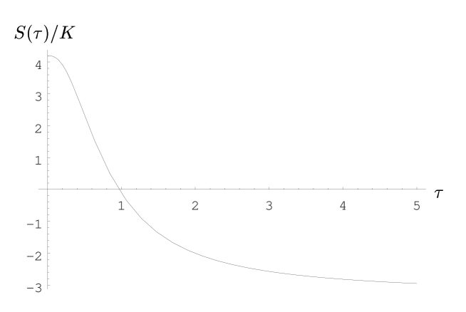
Figure 1: The function $S(\tau)/K$ for the state (6) when $q_{0}=1$ and $p_{0}=-1$. It clearly can become negative, a result which should not be possible for a nonnegative Wigner distribution. This indicates a fault in Bell’s argument.

According to Bell, $F(\tau)$ expresses the probability of $q_{1}$ and $q_{2}$ having different signs, apart from an “unimportant constant” $K$ [20]. However, this conclusion is not straightforward, due to the following argument which applies both to the state considered by Bell in Ref. [20] and the state considered here. A probability can never exceed unity, but we see that $F(\tau)\rightarrow\infty$ as $\tau\rightarrow\infty$. Thus, in order to have a finite probability as $t\rightarrow\infty$, the normalization constant $K$ must approach infinity as $t\rightarrow\infty$. If we now assume that the normalization constant $K$ is time independent, the probability will vanish for all finite times. This is clearly wrong, and besides does not lead to any violation of Bell’s inequality (16). We therefore see that the normalization constant $K$ must depend on time. In the inequality (16), the probability is compared at two different times, and one is not allowed to assume that $K$ is time independent. The conclusion is that the assumption that $K$ is an “unimportant constant” is wrong, and that violation of local realism has not been demonstrated in Ref. [20].

To summarize, it has been found that Bell’s demonstration in Ref. [20] of violation of local realism in phase space for continuous variables is untenable. Bell’s calculation was repeated, but with a nonnegative Wigner function. Nevertheless, it was seemingly possible to derive a violation of local realism. This should not be possible, since a nonnegative Wigner function can be regarded as a local hidden variable theory. It was seen that the error was caused by the use of an unnormalizable state. In this experiment, the two “local times” $t_{k}$ play the role of local parameters in the same way that the orientation of the spin-filters are the local parameters in the standard Bell experiment [1]. It is not permissible to disregard a normalization constant which depends on the local parameters.

References

- [1] J. S. Bell, Physics (Long Island City, N.Y.) 1 (1964) 195.
- [2] J. F. Clauser, M. A. Horne, A. Shimony, and R. A. Holt, Phys. Rev. Lett. 23 (1969) 880 .
- [3] J. F. Clauser and M. A. Horne, Phys. Rev. D 10 (1974) 526.
- [4] N. Gisin and A. Peres, Phys. Lett. A 162 (1992) 15.
- [5] D. M. Greenberger, M. A. Horne, and A. Zeilinger, in: Bell’s Theorem, Quantum Theory and Conceptions of the Universe, ed. M. Kafatos (Kluwer Academic Publishers, Dordrecht, 1989) p. 69.
- [6] L. Hardy, Phys. Rev. Lett. 68 (1992) 2981.
- [7] A. Aspect, P. Grangier, and G. Roger, Phys. Rev. Lett. 47 (1981) 460
- [8] R. Y. Chiao, P. G. Kwiat, and A. M. Steinberg, Quant. Semiclass. Opt. 7 (1995) 259.
- [9] J. F. Clauser and A. Shimony, Rep. Prog. Phys. 41 (1978) 1881.
- [10] F. M. Pipkin, Adv. At. Mol. Phys. 14 (1978) 281.
- [11] A. Einstein, B. Podolsky, and N. Rosen, Phys. Rev. 47 (1935) 777.
- [12] M. A. Horne and A. Zeilinger, in: Symposium on the Foundations of Modern Physics, eds. P. Lahti and P. Mittelstaedt (World Scientific, Singapore, 1985) p. 435.
- [13] M. Żukowski and J. Pykacz, Phys. Lett. A 127 (1988) 1.
- [14] M. A. Horne, A. Shimony, and A. Zeilinger, Phys. Rev. Lett. 62 (1989) 2209.
- [15] J. G. Rarity and P. R. Tapster, Phys. Rev. Lett. 64 (1990) 2495.
- [16] M. D. Reid and P. D. Drummond, Phys. Rev. Lett. 60, 2731 (1988).
- [17] M. D. Reid, Phys. Rev. A 40 (1989) 913.
- [18] Z. Y. Ou, S. F. Pereira, H. J. Kimble, and K. C. Peng, Phys. Rev. Lett. 68 (1992) 3663.
- [19] Z. Y. Ou, S. F. Pereira, and H. J. Kimble, Appl. Phys. B 55 (1992) 265.
- [20] J. S. Bell, in: New Techniques and Ideas in Quantum Measurement Theory, ed. D. M. Greenberger (The New York Academy of Sciences, New York, 1986) p. 263.
- [21] J. S. Bell, Speakable and unspeakable in quantum mechanics (Cambridge University Press, Cambridge, 1987) p. 196.
- [22] E. Wigner, Phys. Rev. 40 (1932) 749.
- [23] U. Leonhardt, Phys. Lett. A 182 (1993) 195.
- [24] U. Leonhardt and J. A. Vaccaro, J. Mod. Opt. 42 (1995) 939.
- [25] A. Peres, Quantum Theory: Concepts and Methods (Kluwer Academic Publishers, Dordrecht, 1993) p. 80.
- [26] D. F. Walls and G. J. Milburn, Quantum Optics (Springer-Verlag, Berlin, 1994) p. 64.
- [27] N. Bohr, Phys. Rev. 48 (1935) 696.