Quantum chaos in an ion trap: the delta-kicked harmonic oscillator

Abstract

We propose an experimental configuration, within an ion trap, by which a quantum mechanical delta-kicked harmonic oscillator could be realized, and investigated. We show how to directly measure the sensitivity of the ion motion to small variations in the external parameters.

PACS: 05.45.+b, 03.65.Bz, 42.50.Vk

In classical mechanics, deterministic chaos is often most simply described as exponential sensitivity to initial conditions, meaning that initially neighbouring classical trajectories diverge extremely rapidly with time. Due to the necessity of preserving the inner product, this kind of divergence between two possible initial states cannot occur quantum mechanically. The question of what then constitutes the quantum mechanical equivalent of chaos immediately arises. An interesting proposal by Peres [1] is to examine the initial state $|\psi\rangle$ evolving under two slightly differing (classically chaotic) Hamiltonians $\hat{H}_{1}$ and $\hat{H}_{2}$. Defining $U_{1,2}(t)$ as the corresponding unitary evolution operators, the overlap

$$O=\left|\langle\psi|U_{2}(t)^{\dagger}U_{1}(t)|\psi\rangle\right|^{2}$$ (1)

is predicted to behave very differently, depending on whether the initial state is in a stable or chaotic area of phase space. Thus $O$ is a measure to distinguish between regular and irregular quantum dynamics. In fact much work on the subject of quantum chaos has been carried out theoretically; experimental realizations however remain somewhat scarce [2], although there have recently been pioneering successes in atom optics [3] and in mesoscopic solid state systems [4]. In this Letter we propose a realizable experimental configuration, with which one can measure $O$ directly. The system proposed is a single ion trapped in a harmonic potential, subject to periodic kicks from a standing wave laser. This is a quantum delta-kicked harmonic oscillator, a system capable classically of stochastic dynamics, including Arnol’d diffusion [5] under certain resonance conditions [6].

Trapped ions are in many ways an ideal choice of system for the study of fundamental aspects of quantum mechanics. One can take advantage of the small dissipation in this system, together with the possibility of coherent manipulation of the ion’s motional state. Trapped ions have been used in recent experimental demonstrations of the generation of non-classical states of motion [7], quantum logic gates [8], and tomography of the density matrix [9]. In addition there have been theoretical proposals for investigation of localization [10] and irregular collapse and revival dynamics [11] due to quantum chaos in this system.

In this Letter we will first describe a general procedure for determining $O$ as a function of time. We then describe explicitly a particular system, the delta-kicked harmonic oscillator, how it may be implemented within an ion trap, and how to carry out our general procedure for determining $O$. Finally we display some numerical results, showing what one would expect to see when carrying out such an experiment. Markedly different results are indeed observed numerically, dependent on whether the initial condition is in a classically stable or chaotic area of phase space.

We first consider a general Hamiltonian of the form $\hat{H}=\hat{H}_{1}|g_{1}\rangle\langle g_{1}|+\hat{H}_{2}|g_{2}\rangle\langle g_{2}|,$ where $|g_{1}\rangle$ and $|g_{2}\rangle$ are stable electronic ground states of a single trapped ion. The state of the ion is set initially to be:

$$|\psi(0)\rangle=\frac{1}{\sqrt{2}}\left(|g_{1}\rangle|\alpha\rangle+|g_{2}\rangle|\beta\rangle\right).$$ (2)

Here $|\alpha\rangle$ and $|\beta\rangle$ are states of the ion’s motion. In the applications described in this Letter, $|\alpha\rangle$ and $|\beta\rangle$ are coherent states; $|\psi(0)\rangle$ is then a Schrödinger cat state, which has been achieved experimentally for a trapped ion [7]. After a time $t$, the initial state evolves to $|\psi(t)\rangle=[|g_{1}\rangle\hat{U}_{1}(t)|\alpha\rangle+|g_{2}\rangle\hat{U}_{2}(t)|\beta\rangle]/\sqrt{2},$ where $\hat{U}_{1}(t)$ and $\hat{U}_{2}(t)$ are the time evolution operators derived from $\hat{H}_{1}$ and $\hat{H}_{2}$, respectively. A $\pi/2$ pulse is applied (Ramsey type experiment) to the ion, yielding

$$|\psi(t)\rangle^{\prime} = \frac{1}{2}\left\{|g_{1}\rangle\left[\hat{U}_{1}(t)|\alpha\rangle-\hat{U}_{2}(t)|\beta\rangle\right]+\right.$$ (4)

$$\left.|g_{2}\rangle\left[\hat{U}_{1}(t)|\alpha\rangle+\hat{U}_{2}(t)|\beta\rangle\right]\right\}.$$

The probability for the ion to be in state $|g_{1}\rangle$ is thus

$$P_{g}=\frac{1}{2}\left\{1-\mbox{Re}\left[\langle\beta|\hat{U}_{2}^{\dagger}(t)\hat{U}_{1}(t)|\alpha\rangle\right]\right\}.$$ (5)

Similarly, if we set $|\psi(0)\rangle=(|g_{1}\rangle|\alpha\rangle+i|g_{2}\rangle|\beta\rangle)/\sqrt{2},$ the corresponding final probability is given by

$$P_{g}^{\prime}=\frac{1}{2}\left\{1-\mbox{Im}\left[\langle\beta|\hat{U}_{2}^{\dagger}(t)\hat{U}_{1}(t)|\alpha\rangle\right]\right\}.$$ (6)

By determining $P_{g}$ and $P_{g}^{\prime}$, one can clearly deduce $|\langle\beta|\hat{U}_{2}^{\dagger}(t)\hat{U}_{1}(t)|\alpha\rangle|^{2}.$ If $\hat{H}_{1}$ and $\hat{H}_{2}$ are slightly differing chaotic Hamiltonians, and $|\alpha\rangle=|\beta\rangle$, then we have $O$, as defined in Eq. (1). We also note that where $\hat{H}_{2}$ is the simple harmonic oscillator Hamiltonian, this collapses to $2\pi Q(\beta)$, where $Q(\beta)$ is the $Q$ function for various initial $\beta$ of the pure state $\hat{U}_{1}(t)|\alpha\rangle$. By repeated measurements one can therefore determine the $Q$ function’s evolution in time [12].

Our proposed model system is a harmonic oscillator

$$H_{0}=\frac{p^{2}}{2m}+\frac{m\nu^{2}x^{2}}{2},$$ (7)

periodically perturbed by nonlinearly position-dependent delta-kicks;

$$H_{1}=K\cos(kx)\sum_{n=-\infty}^{\infty}\delta(t-n\tau),$$ (8)

so that $H=H_{0}+H_{1}$. Here $x$ is the position, $p$ the momentum, $m$ the mass, $\nu$ the oscillator frequency, $k=2\pi/\lambda$ the wavenumber, $t=$ time, $\tau$ the time delay between the kicks, and $K$ the kick strength. Under the resonance condition $\nu\tau=2\pi r/q$ ($r/q$ is a positive rational, where $q>2$), classically there are thin channels of chaotic dynamics in the phase space [6]. The resulting Arnol’d stochastic web [see Fig. 1(a)] spreads through all of phase space; Arnol’d diffusion [5] can occur in systems of less than two dimensions when the conditions for the KAM (Kolmogorov, Arnol’d, Moser) theorem [13] are not fulfilled, as is the case here [6]. The corresponding quantum mechanical system has also been studied theoretically [14] [see Figs. 1(b,c,d) for the time averaged $Q$ function of this system].

To construct such a system quantum mechanically, which can also be used to carry out the procedure described in Eqs. (4,5,6), we begin with a single ion in a harmonic potential (e.g. a linear ion trap [7]); in addition we require a time dependent standing wave laser configuration. The ion has two ground states and two excited states, and the laser is elliptically polarized [see Fig. 2(a)]. The $\sigma_{+}$ and $\sigma_{-}$ polarized contributions thus separately couple two different two level systems, with different Rabi frequencies:

$$\hat{H} = \hat{H}_{0}+\frac{\hbar}{2}\sum_{j=1}^{2}\left\{\omega_{0}(|e_{j}\rangle\langle e_{j}|-|g_{j}\rangle\langle g_{j}|)\right.$$ (10)

$$\left.+\cos(k\hat{x})\left[\Omega_{j}(t)e^{-i\omega_{L}t}|e_{j}\rangle\langle g_{j}|+\mbox{H.c.}\right]\right\},$$

where $\omega_{0}$ is the transition frequency between the electronic states $|e_{j}\rangle$ and $|g_{j}\rangle$, $\omega_{L}$ is the laser frequency, and $\Omega_{1,2}(t)$ are the (time dependent) Rabi frequencies. In a rotating frame defined by $\hat{U}=\exp[-i\omega_{L}t\sum_{j=1}^{2}(|e_{j}\rangle\langle e_{j}|-|g_{j}\rangle\langle g_{j}|)/2]$, and in the limit of large detuning $|\Delta|=|\omega_{L}-\omega_{0}|\gg|\Omega_{1,2}(t)|$, $|e_{1}\rangle$ and $|e_{2}\rangle$ can be adiabatically eliminated to give:

$$\hat{H}=\hat{H}_{0}+\frac{\hbar}{8\Delta}\sum_{j=1}^{2}\Omega_{j}(t)^{2}\left[\cos\left(2k\hat{x}\right)+1\right]|g_{j}\rangle\langle g_{j}|.$$ (11)

The laser is rapidly and periodically switched, giving a series of short Gaussian pulses:

$$\Omega_{j}(t)^{2}=\Omega_{j}^{2}\sum_{n=-\infty}^{\infty}e^{-(t-n\tau)^{2}/\sigma^{2}},$$ (12)

which approximate a series of delta kicks in the limit $\sigma\rightarrow 0$. Note also that we require $\sigma\gg 1/\Delta$, otherwise the laser is too spectrally broad, making adiabatic elimination of $|e_{1}\rangle$ and $|e_{2}\rangle$ impossible. Thus, finally, we have:

$$\hat{H}=\hat{H}_{0}+\sum_{j=1}^{2}K_{j}\left[\cos\left(2k\hat{x}\right)+1\right]|g_{j}\rangle\langle g_{j}|\sum_{n=-\infty}^{\infty}\delta(t-n\tau),$$ (13)

which corresponds almost exactly to Eqs. (7,8), for two different $K_{j}=\hbar\sigma\sqrt{\pi}\Omega_{j}^{2}/8\Delta$. There are extra $|g_{j}\rangle\langle g_{j}|$ terms, but these will only contribute phases to the evolution of the initial state of Eq. (2), and can easily be accounted for.

Taking $|\alpha\rangle=|\beta\rangle$, the initial state of Eq. (2) thus evolves as

$$|\psi(n\tau)\rangle=\frac{1}{\sqrt{2}}\sum_{j=1}^{2}e^{-in\kappa_{j}/\sqrt{2}{\eta}^{2}}\hat{F}_{j}^{n}|g_{j}\rangle|\alpha\rangle$$ (14)

where the Floquet time evolution operators $\hat{F}_{j}$ are given by:

$$\hat{F}_{j}=e^{-i\hat{a}^{\dagger}\hat{a}\nu\tau}e^{-i\kappa_{j}\cos[2\eta(\hat{a}^{\dagger}+\hat{a})]|g_{j}\rangle\langle g_{j}|/\sqrt{2}{\eta}^{2}},$$ (15)

where $\hat{a}^{\dagger}$ and $\hat{a}$ respectively create and annihilate a single phonon quantum, and the common phase term $e^{-i\nu\tau/2}$ has been dropped. The $\kappa_{j}=\Omega_{j}^{2}{\eta}^{2}\sigma\sqrt{2\pi}/8\Delta$ are dimensionless kick parameters, which, with $\nu\tau$, determine fully the phase space behaviour of the classical delta-kicked harmonic oscillator [6]. In the quantum mechanical problem there is an additional parameter, the Lamb-Dicke parameter $\eta=k\sqrt{\hbar/2m\nu}$. As $\eta^{2}\propto\hbar$, by progressively reducing $\eta$, one can explore the transition from quantum to classical chaos [15]. This can be accomplished by “tightening” or “loosening” the trapping potential, i.e. increasing or decreasing the trapping frequency $\nu$.

After $n$ kicks, we perform a $\pi/2$ pulse between the levels $|g_{1}\rangle$ and $|g_{2}\rangle$, by e.g. a Raman transition or a magnetic field [see Fig. 2(b)]. By fluorescence, using an auxiliary level $|f\rangle$, with repeated measurements one can determine $P_{g}$ and $P_{g}^{\prime}$ [see Fig. 2(c)], as defined in Eqs. (5,6).

$$P_{g} = \frac{1}{2}\left[1-\cos(\delta\kappa n/\sqrt{2}{\eta}^{2})\mbox{Re}\left(\langle\alpha|\hat{F}_{2}^{\dagger n}\hat{F}_{1}^{n}|\alpha\rangle\right)-\right.$$ (17)

$$\left.\sin(\delta\kappa n/\sqrt{2}{\eta}^{2})\mbox{Im}\left(\langle\alpha|\hat{F}_{2}^{\dagger n}\hat{F}_{1}^{n}|\alpha\rangle\right)\right]$$

$$P_{g}^{\prime} = \frac{1}{2}\left[1-\sin(\delta\kappa n/\sqrt{2}{\eta}^{2})\mbox{Re}\left(\langle\alpha|\hat{F}_{2}^{\dagger n}\hat{F}_{1}^{n}|\alpha\rangle\right)-\right.$$ (19)

$$\left.\cos(\delta\kappa n/\sqrt{2}{\eta}^{2})\mbox{Im}\left(\langle\alpha|\hat{F}_{2}^{\dagger n}\hat{F}_{1}^{n}|\alpha\rangle\right)\right],$$

where $\delta\kappa=\kappa_{2}-\kappa_{1}$. From Eq. (17) one can easily extract the overlap $O=|\langle\alpha|\hat{F}_{2}^{\dagger n}\hat{F}_{1}^{n}|\alpha\rangle|^{2}$.

In order to relate the quantum mechanical behavior of the system to the classical one, we have to use an initial condition equivalent to the classical $x(0)$ and $p(0)$. We use a coherent state $|\alpha\rangle$, where $\alpha$ can be expressed as $\alpha=[kx(0)+ikp(0)/m\nu]/4\eta$. Thus we can see that when $\eta$ is small, $\alpha$ is large, and $|\alpha\rangle$ is therefore more macroscopic, in some sense more classical. This can be seen by comparing Fig. 1(c) with Fig. 1(d); for $\eta=0.5$ population “tunnels” through a classically forbidden area, which does not occur when $\eta=0.25$ [16].

Figure 3 shows the values of $P_{g}$ and $P_{g}^{\prime}$ that one would measure for this scheme, and the value of $O$ that one would thus obtain, for $\eta=0.5$ after $0$–$1000$ kicks. The plots obtained are clearly different, depending on whether the initial condition is classically unstable, as in Figs. 3(a,b) where the corresponding classical initial condition is a hyperbolic fixed point, or stable [Figs. 3(c,d), elliptic fixed point]. This is already noticeable in the plots of $P_{g}$ and $P_{g}^{\prime}$, before $O$ is extracted [Figs. 3(a,c)]. In line with previous numerical work for the kicked top [1], $O$ decays for an unstable initial condition, and undergoes quasistable oscillations for a stable initial condition.

As $O$ is a measure of how close the two parallel evolutions are at a given time, it can be seen that if the initial condition is classically unstable [Fig. 3(b)] the two states become rapidly increasingly orthogonal (more “far apart”), whereas in the case of a stable initial condition, for some time the difference between the states remains on average about the same. This in some sense corresponds to the classical definition of chaos, where under the influence of the same dynamics, very slightly different initial states diverge rapidly if their origin is in an unstable area of phase space [1].

Figure 4 shows the same for $\eta=0.25$. In line with the fact that this is more in the semiclassical regime than Fig. 3, the decay [Figs. 4(a,b)] is more rapid, and the oscillations [Figs. 4(c,d)] are more stable. The slow decay of the quasistable oscillations when $\eta=0.5$ [Fig. 3(d)] can be traced back to the tunneling that takes place in this regime (see Fig. 1), absent when $\eta=0.25$.

Numerically the procedure is carried out in a truncated Fock basis of 400 states when $\eta=0.5$, or 800 when $\eta=0.25$. Increasing the size of the Fock basis does not qualitatively change the observed dynamics.

In conclusion we have shown a general procedure for determining the overlap parameter $O$ originally proposed by Peres [1]. We have described explicitly how $O$ could be determined for the delta-kicked harmonic oscillator, a classically chaotic system. We have described how a single ion trapped in a harmonic potential could be a practical experimental realization of the delta-kicked harmonic oscillator, and how our scheme for determining $O$ is realized in this configuration. In particular, our scheme presents a direct way for determining $O$, by virtue of the fact that we effectively have two Hamiltonians running in parallel, within the same experimental system.

We thank R. Blatt, J. Eschner, P. Gerwinski, F. Haake, J. P. Paz, W. P. Schleich, H. Schomerus, P. Törmä, D. J. Wineland, and W. H. Zurek for discussions. This work was supported by the Austrian Fond zur Förderung der wissenschaftlichen Forschung and TMR network ERBFMRX-CT96-0002.

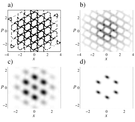
FIG. 1.: Stroboscopic Phase space portraits (from kick to kick) for the delta-kicked harmonic oscillator, where $r/q=1/6$ and $\kappa=0.2$, after averaging over $11000$ kicks. The position $x$ and momentum $p$ axes are in units of $\lambda$ and $m\nu\lambda$ respectively. (a) Poincaré surface of section, showing the classical stochastic web. Regular dynamics take place within the cells defined by the web. (b) Time averaged $Q$ function for the (unstable) initial condition $|\alpha\rangle$ where $\alpha=\pi/2\eta$ and $\eta=0.25$, centred at $(1,0)$. (c) Time averaged $Q$ function for the (stable) initial condition $\alpha=i\pi/\eta{\sqrt{3}}$ ($(0,2/{\sqrt{3}})$) and $\eta=0.5$. (d) As for (c), where $\eta=0.25$. Note the “tunneling” out of the original ring of cells for the larger value of $\eta$.

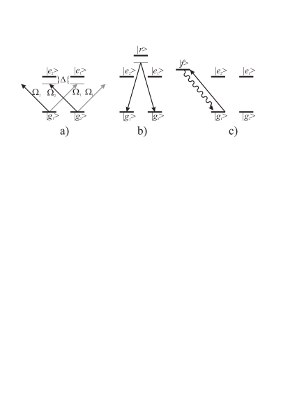
FIG. 2.: Atomic level configuration proposed for our procedure. (a) The atom first experiences a series of short laser pulses from an elliptically polarized standing wave. Levels $|g_{1}\rangle$ and $|e_{1}\rangle$ are coupled by $\sigma_{+}$polarized light, and levels $|g_{2}\rangle$ and $|e\rangle$ by $\sigma_{-}$ polarized light, where the corresponding intensities differ. (b) After a definite number of kicks, the levels $|g_{1}\rangle$ and $|g_{2}\rangle$ experience a $\pi/2$ pulse (e.g. a Raman transition, using the auxiliary level $|r\rangle$). (c) The population of $|g_{1}\rangle$ is determined by fluorescence, using the auxiliary level $|f\rangle$.

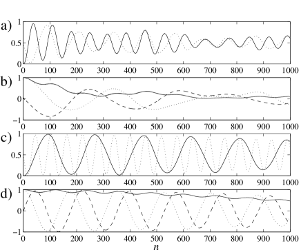
FIG. 3.: (a) $P_{g}$ (solid line) and $P_{g}^{\prime}$ (dotted line) for the initial condition $\alpha=\pi/2\eta$ ($\eta=0.5$, $\kappa_{1}=0.2$, $\kappa_{2}=0.225$). (b) $O$ (solid line), $\mbox{Re}(\langle\alpha|\hat{F}_{-}^{n\dagger}\hat{F}_{+}^{n}|\alpha\rangle)$ (dashed line), and $\mbox{Im}(\langle\alpha|\hat{F}_{-}^{n\dagger}\hat{F}_{+}^{n}|\alpha\rangle)$ (dotted line) for the same initial condition. (c) and d), same as a) and b), for the initial condition $\alpha=i\pi/\eta{\sqrt{3}}$.

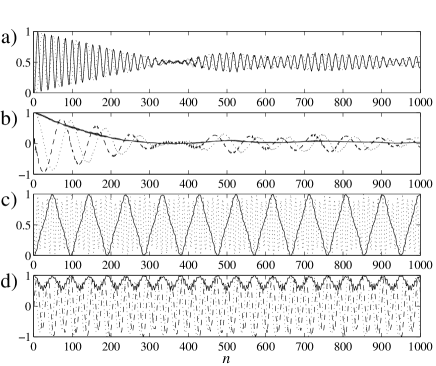
FIG. 4.: Corresponds exactly to Fig. 3, except that $\eta=0.25$

REFERENCES

- [1] A. Peres, in Quantum Chaos: Proceedings of the Adriatico Research Conference on Quantum Chaos, edited by H. A. Cerdeira et al., (World Scientific, Singapore, 1991); see also A. Peres, Quantum Theory: Concepts and Methods (Kluwer Academic Publishers, Dordrecht 1993); F. Haake, Quantum Signatures of Chaos (Springer-Verlag, Berlin 1991).
- [2] E. Doron, U. Smilansky, and A. Frenkel, Phys. Rev. Lett. 65, 3072 (1990); J. E. Bayfield et al., Phys. Rev. Lett. 63, 364 (1989); E. J. Galvez et al., Phys. Rev. Lett. 61, 2011 (1988); for a review on microwave driven hydrogen experiments, see P. M. Koch and K. A. H. van Leeuwen, Phys. Rep. 255, 289 (1995).
- [3] F. L. Moore et al., Phys. Rev. Lett. 75, 4598 (1995); J. C. Robinson et al., Phys. Rev. Lett. 74, 3963 (1995); F. L. Moore et al., Phys. Rev. Lett. 73, 2974 (1994).
- [4] P. B. Wilkinson et al., Nature 380, 608 (1996); T. M. Fromhold et al., Phys. Rev. Lett. 75, 1142 (1995).
- [5] V. I. Arnol’d, Sov. Math. Doklady 5, 581 (1964).
- [6] A. A. Chernikov et al., Computers Math. Applic. 17, 17 (1989); V. V. Afanasiev et al., Phys. Lett. A 144, 229 (1990); see also L. E. Reichl The Transition to Chaos (Springer-Verlag, New York 1992).
- [7] D. M. Meekhof et al., Phys. Rev. Lett. 76, 1796 (1996); C. Monroe et al., Science 272, 1131 (1996); for theoretical proposals of nonclassical states see J. I. Cirac et al., Adv. At. Mol. Phys. 37, 237 (1996).
- [8] C. Monroe et al., Phys. Rev. Lett. 75, 4714 (1995); for a theoretical proposal see J. I. Cirac and P. Zoller, Phys. Rev. Lett., 74, 4091 (1995).
- [9] D. Leibfried et al., Phys. Rev. Lett. 77, 4281 (1996); for theoretical proposals see S. Wallentowitz and W. Vogel Phys. Rev. Lett. 75, 2932 (1995); J. F. Poyatos et al., Phys. Rev. A 53 R1966; C. D’Helon and G. J. Milburn, Phys. Rev. A 54, R25 (1996).
- [10] M. El Ghafar et al., Phys. Rev. Lett. 78, 4181 (1997).
- [11] J. K. Breslin, C. A. Holmes, and G. J. Milburn, Phys. Rev. A 56, 3022 (1997).
- [12] See also L. G. Lutterbach and L. Davidovich, Phys. Rev. Lett. 78, 2547 (1997).
- [13] A. N. Kolmogorov, Dokl. Akad. Nauk. SSSR 98, 527 (1954); V. I. Arnol’d, Russ. Math. Survey 18, 9, 85 (1963); J. Moser, Nachr. Akad. Wiss. Göttingen II, Math. Phys. Kl. 18, 1 (1962); see also L. E. Reichl The Transition to Chaos (Springer-Verlag, New York 1992).
- [14] G. P. Berman, V. Yu. Rubaev, and G. M. Zaslavsky, Nonlinearity 4, 543 (1991); M. Frasca, Phys. Lett. A 231, 344 (1997), and references therein.
- [15] R. Graham, M. Schlautmann, and P. Zoller, Phys. Rev. A 45, R19 (1992); for an experiment on localization in a standing light wave see [3].
- [16] The tunneling effect can be measured by tomographic methods (see [9, 12]). One can also also observe the tunneling to the center of the web using the present scheme with in Eq. (2) and the free evolution of the harmonic oscillator [compare Eqs. (5) and (6)].