1.4

Approximate Consistency and Prediction Algorithms in Quantum Mechanics J. N. McElwaine
Clare College, Cambridge

A dissertation submitted for the degree of Doctor of Philosophy
University of Cambridge

October 1996

Abstract

This dissertation investigates questions arising in the consistent histories formulation of the quantum mechanics of closed systems. Various criteria for approximate consistency are analysed. The connection between the Dowker-Halliwell criterion and sphere packing problems is shown and used to prove several new bounds on the violation of probability sum rules. The quantum Zeno effect is also analysed within the consistent histories formalism and used to demonstrate some of the difficulties involved in discussing approximate consistency. The complications associated with null histories and infinite sets are briefly discussed.

The possibility of using the properties of the Schmidt decomposition to define an algorithm which selects a single, physically natural, consistent set for pure initial density matrices is investigated. The problems that arise are explained, and different possible algorithms discussed. Their properties are analysed with the aid of simple models. A set of computer programs is described which apply the algorithms to more complicated examples.

Another algorithm is proposed that selects the consistent set (formed using Schmidt projections) with the highest Shannon information. This is applied to a simple model and shown to produce physically sensible histories. The theory is capable of unconditional probabilistic prediction for closed quantum systems, and is strong enough to be falsifiable. Ideas on applying the theory to more complicated examples are discussed.

Declaration

The research reported in this dissertation was carried out in the Department of Applied Mathematics and Theoretical Physics at the University of Cambridge between October 1993 and September 1996. It is original except where explicit reference is made to the work of others. Chapters 3 and 4 describe work done in collaboration with Adrian Kent [1]. Chapter 2 is largely the same as [2], and chapter 6 and part of chapter 4 are similar to [3]. No part of the dissertation has been or is being submitted for any degree or other qualification at any other university.

Chapter 1 General introduction

1.1 Quantum mechanics

Quantum mechanics is a tremendously successful theory that makes predictions with unprecedented accuracy. The standard Copenhagen interpretation has existed since the 1920’s [4, 5, 6] and has passed every experimental test. However, it occupies a very unusual place among physical theories: it contains classical mechanics as a limiting case, yet at the same time it requires this limiting case for its own interpretation [7, 8, 9].

In the beginning quantum mechanics was only tested on microscopic systems, though some part of it works well for macroscopic systems; superconductivity, superfluidity, neutron stars and lasers are all examples where macroscopic behaviour depends on intrinsically quantum effects. Today, however, experiments involving SQUIDS (Superconducting Quantum Interference Devices) and other systems [10, 11, 12, 13, 14, 15, 16, 17] aim to create superpositions of macroscopically distinct states and detect interference between them, and in quantum cosmology quantum mechanics is being applied to the entire universe. Both these areas lie outside the realm of the Copenhagen interpretation, but the difficulties are particularly acute in quantum cosmology, since there are no external systems and it is highly unlikely that any systems obeying classical mechanics existed in the early universe. The Copenhagen interpretation also suffers from being defined in vague terms: what is an observer, an observable or a measurement? After seventy years there is still no consensus, and this suggests to us that quantum mechanics is incomplete.

We feel that a quantum theory should describe an objective reality independent of observers and that it should be mathematically precise. That is, given a closed quantum system the theory should make exact predictions for the set of possible outcomes and their probabilities. It seems to us important that the theory should be applicable to individual systems and require no reference to objects outside the system — how else can a theory of quantum cosmology be understood? We discuss below some of the current programs that seek to extend the Copenhagen approach and remove its ambiguities, and see how they measure up to these desiderata.

Current approaches to quantum mechanic can be divided up into those that are incompatible with Copenhagen quantum mechanics — in the sense that they fundamentally alter the dynamics of quantum mechanics and hence make different predictions in some situations — and those that are compatible with Copenhagen quantum mechanics — in the sense that they have the same fundamental dynamics as quantum mechanics so that they always agree with the probabilistic predictions of Copenhagen quantum mechanics, though there may be additional variables and dynamical equations and they may make additional predictions.

Among the attempts at compatible theories is the very popular idea of a many-worlds interpretation, which was introduced by Everett [18] and has been extensively studied [19, 20, 21, 22]. We feel the most important criticism of these ideas is not a prejudice against multiple branching universes, but that no precise formulation of it has yet been made that is capable of making predictions [23, 24, 25, 26]. This problem — the problem of specifying what constitutes an event and which basis to use — recurs in many approaches to quantum mechanics.

The de Broglie-Bohm pilot wave theory [27] is compatible. It is a realistic theory that introduces the positions of particles as hidden variables and it continues to attract interest [28, 29, 30, 31, 32, 33, 34, 35, 36, 37]. As a result of the privileging of the position variables quasiclassical dynamics becomes a corollary of the theory and this approach undoubtedly solves some of the problems of the Copenhagen interpretation. However, despite much effort, attempts to produce a relativistic theory have failed, so though it satisfies our desiderata when applied to non-relativistic quantum mechanics no relativistic theory exists. In fact, it seems to us that the theory is intrinsically incapable of a relativistic extension since it involves action at a distance and ascribes unbounded velocities to particles.

The de Broglie-Bohm pilot wave theory, as Bell explains [38], highlights the flaws in the assumptions of the no-hidden-variables proofs of Von Neumann and others [5, 39, 40]. Realistic, complete, hidden-variables theories (such as de Broglie-Bohm) do exist, but his later work [41], on the EPR (Einstein-Podolsky-Rosen) paradox, shows that such theories must be nonlocal — in the sense that measurements on one system can effect a distant system that it interacted with in the past. His proof shows that certain inequalities (referred to as Bell’s inequalities) are satisfied by quantum mechanics but not by any local hidden-variables theory, if, roughly speaking, the experimenter can independently specify the experiment. Bell’s inequalities have been experimentally validated [42, 43] and Bell’s conclusions have recently been extended by Greenberger et. al. [44, 45]. They consider three spin half particles and prove the stronger result that there is a direct (rather than statistical) contradiction between the EPR axioms (completeness, reality, locality) and quantum mechanics.

A realistically interpretable, relativistically invariant theory has been described by Samols [46] on a 2d light-cone lattice. His theory is operationally indistinguishable from standard quantum theory, though whether this model can usefully be applied to physical examples is unclear. There is also the question of whether some suitable continuum limit exists.

In their seminal work [47] Ghirardi, Rimini and Weber rekindled interest in stochastic collapse models. Their original theory supplements the Schrödinger equation with a stochastic process — their theory is incompatible with quantum mechanics. Their ideas have been developed into a family of theories [48, 49, 50, 51, 52, 53, 54, 55, 56, 57, 58, 59, 60, 61] in which defects with the original proposal have been removed and extensions have been made to so called continuous localisation models where the individual jumps become infinitesimal and the states undergo quantum state diffusion.

Ghirardi, Rimini and Weber’s original proposal was that for each particle there was a probability of $1/\tau$ ($\tau\approx 10^{15}\mbox{s}$) per unit term of it undergoing “wave-function” collapse. These collapses take place about a randomly chosen point (probability density function given by $|\psi|^{2}$) and after the collapse the new wave function is Gaussian (in the collapsed coordinate) with characteristic length $a\approx 10^{-7}\mbox{m}$. In their approach the state vector can be interpreted realistically — the state vector is precisely the current physical state — but its Hamiltonian evolution is altered by coupling it to a stochastic field. The individual collapse centres can also be regarded as the ontology of the theory [62].

The stochastic collapse approach has many desirable features. There is no need for ill-defined concepts such as measurement, observers, system or apparatus, and the theory can be successfully applied to closed systems. A preferred basis must be chosen (usually position eigenstates) but it is precisely given. The preferred basis defines an operator that couples the wavefunction to the stochastic field such that the wavefunction evolves into an eigenvector of the preferred operator. Quantum state diffusion has been suggested as a fundamental theory but attempts to make these ideas relativistically invariant have failed [63] — though perhaps Pearle’s latest theory [64] solves some of the problems. These theories also generically violate the conservation of energy and other conserved quantities, though apart from these deficiencies they satisfy all of our desiderata.

Stochastic theories can also be motivated as potentially arising from approximations to a quantum theory of gravity [65, 66, 67, 68, 69, 70, 71, 72, 73, 74]. For example, Penrose [75, 76] believes that as soon as there is a “significant” amount of space-time curvature the rules of quantum linear superposition must fail — that is an event occurs and the wave function “collapses”. By “significant” he means, roughly speaking, when the difference in gravitational fields is one graviton or more. Though these proposals are interesting, without a quantum theory of gravity, or an approximation to one, they cannot be expressed precisely enough to develop a useful theory.

The importance of decoherence is now widely recognised. One of the earliest papers on decoherence was by Mott [77] in 1929. He considered the $\alpha$-decay of nucleus in a cloud chamber and asked why the $\alpha$-particle produced straight line tracks when it was a spherical wave. The answer of course is that decoherence has occured — the different straight line tracks have become entangled with environment states that are approximately orthogonal. Decoherence by interaction with the environment appears to play a fundamental role in the emergence of classical phenomena. These ideas have been studied in a wide range of physical systems in recent years [78, 79, 80, 81, 82, 83, 84, 85, 86, 87, 88]. These papers show that, for a wide range of systems, in a suitable basis, the off-diagonal elements of the reduced density matrix decay exponentially in time.

While the significance of decoherence is uncontroversial some authors claim that the decoherence program contains its own interpretation (see for example [86] and references therein). However, unless some form of non-unitary evolution is proposed this approach seems unsatisfactory as a fundamental theory to us, since a closed system can always be regarded as being in a pure state. Without specifying a preferred basis to use for the reduced density matrix (as well as a split between system and environment) this approach cannot describe the events that take place within a closed system [89, 8, 76].

The consistent histories approach to quantum theory was originally developed by Griffiths [90], Omnès [91], and Gell-Mann & Hartle [92]. Griffiths and Omnès see it as an attempt to remove the ambiguities and difficulties inherent in the Copenhagen interpretation, but Gell-Mann & Hartle are motivated by an attempt to make precise the ideas of a many worlds interpretation in the context of quantum cosmology.

The predictions of the consistent histories formalism are identical to the predictions of standard quantum mechanics where laboratory experiments are concerned, but they take place within a more general theory. The basic objects are sequences of events or histories. A set of histories must include all possibilities and must be consistent. The individual histories can then be considered physical possibilities with definite probabilities, and they obey the ordinary rules of probability and logical inference. The set of projections used and the projection times can be the same for each history in which case the set of histories is called branch-independent. However, there is no reason to expect projections which lead to consistent histories in one branch to be consistent in another: why should projections for the position of the earth be consistent in another branch of the universe where the solar system never formed? When the choice of projections and projection times depend on the earlier projections in a history the set of histories is called branch-dependent.

For the remainder of this dissertation we are going to focus on the consistent histories approach, though some of the results highlight problems that also affect other approaches.

1.2 The consistent histories approach

1.2.1 Consistent histories formalism

Let $\rho$ be the initial density matrix of a quantum system. A branch-dependent set of histories is a set of products of projection operators indexed by the variables $\alpha=\{\alpha_{n},\alpha_{n-1},\ldots,\alpha_{1}\}$ and corresponding time coordinates $\{t_{n},\ldots,t_{1}\}$, where the ranges of the $\alpha_{k}$ and the projections they define depend on the values of $\alpha_{k-1},\ldots,\alpha_{1}$, and the histories take the form:

$$C_{\alpha}=P_{\alpha_{n}}^{n}(t_{n};\alpha_{n-1},\ldots,\alpha_{1})P_{\alpha_{n-1}}^{n-1}(t_{n-1};\alpha_{n-2},\ldots,\alpha_{1})\ldots P_{\alpha_{1}}^{1}(t_{1})\,.$$ (1.1)

Here, for fixed values of $\alpha_{k-1},\ldots,\alpha_{1}$, the $P^{k}_{\alpha_{k}}(t_{k};\alpha_{k-1},\ldots,\alpha_{1})$ define a projective decomposition of the identity indexed by $\alpha_{k}$, so that $\sum_{\alpha_{k}}P^{k}_{\alpha_{k}}(t_{k};\alpha_{k-1},\ldots,\alpha_{1})=1$ and

$$P^{k}_{\alpha_{k}}(t_{k};\alpha_{k-1},\ldots,\alpha_{1})P^{k}_{\alpha^{\prime}_{k}}(t_{k};\alpha_{k-1},\ldots,\alpha_{1})=\delta_{\alpha_{k}\alpha^{\prime}_{k}}P^{k}_{\alpha_{k}}(t_{k};\alpha_{k-1},\ldots,\alpha_{1})\,.$$ (1.2)

These projection operators (hereafter referred to as projections) are the most basic objects in the consistent histories formulation and they represent particular states of affairs existing at particular times [90]. They are combined into time-ordered strings, the class operators $\{C_{\alpha}\}$, which are the elementary events, or histories, in the probability sample space. Here and later, though we use the compact notation $\alpha$ to refer to a history, we intend the individual projection operators and their associated times to define the history.

More general sets of class-operators can be created by coarse-graining. $\mathcal{S}^{*}=\{C^{*}_{\beta}\}$ is a coarse-graining of $\mathcal{S}$ if $C^{*}_{\beta}=\sum_{\alpha\in\overline{\alpha}_{\beta}}C_{\alpha}$, where $\{\overline{\alpha}_{\beta}\}$ is a partition of $\mathcal{S}$. Omnès defines sets of histories without any coarse-graining as Type I, and those which have been coarse-grained but where the class-operators are still strings of projections as Type II [91]. We shall follow Isham [93] and call these class operators homogenous. We follow Gell-Mann and Hartle and use completely general class-operators [94], though on occasion we shall state stronger results which hold for homogenous class-operators.

Probabilities are defined by the formula

$$p(\alpha)=D_{\alpha\alpha},$$ (1.3)

where $D_{\alpha\beta}$ is the decoherence matrix

$$D_{\alpha\beta}=\mbox{Tr}\,(C_{\alpha}\rho C_{\beta}^{\dagger})\,.$$ (1.4)

If no further conditions were imposed these probabilities could contradict ordinary quantum mechanics: they would be inconsistent. In Griffiths’ and Omnès’ original papers [90, 91] they impose the consistency criterion that probability sum rules must be satisfied for all coarse grainings that result in homogenous histories. They show that the necessary and sufficient condition is that

$$p(\alpha+\beta)=p(\alpha)+p(\beta),\quad\forall\alpha\neq\beta\mbox{~{}s.t.\ $(\alpha+\beta)$ is a homogenous history,}$$ (1.5)

which, from eq. (1.3), is equivalent to

$$\mbox{Re}\,(D_{\alpha\beta})=0,\quad\forall\alpha\neq\beta\mbox{~{}s.t.\ $(\alpha+\beta)$ is a homogenous history.}$$ (1.6)

A slightly stronger and more convenient criterion is that probability sum rules should be satisfied for all coarse grainings. The necessary and sufficient criterion in this case is [92]

$$\mbox{Re}\,(D_{\alpha\beta})=0,\quad\forall\alpha\neq\beta,$$ (1.7)

which Gell-Mann and Hartle call weak consistency. A stronger condition,

$$D_{\alpha\beta}=0,\quad\forall\alpha\neq\beta,$$ (1.8)

is often used in the literature for simplicity, which Gell-Mann and Hartle call medium consistency. Gell-Mann and Hartle define two stronger criteria in [94] and more recently yet another [95]. In physical examples they usually are equivalent so we restrict ourselves to the weak (1.7) or medium (1.8) criterion according to which is more convenient.

There are at least two other criteria that have also been proposed. Kent defines [96] an ordered consistent set to be a consistent set of histories $\mathcal{S}$ such that

$$p(\alpha)\leq p(\beta)\mbox{~{}for all $\alpha\leq\beta$, $\alpha$ in some consistent set and $\beta\in\mathcal{S}$,}$$ (1.9)

where $\alpha\leq\beta$ means that every projection in history $\alpha$ projects onto a subspace of the corresponding projection in history $\beta$. Kent shows that ordered consistency defines a more strongly predictive version of the consistent histories formulation that avoids the problems of contrary inferences.

A weaker generalisation is due to Goldstein and Page [97]. They define the probability of a history $\alpha$ by

$$p(\alpha)=\mbox{Re Tr}\,(C_{\alpha}\rho)\quad\mbox{whenever $\mbox{Re Tr}\,(C_{\alpha}\rho)\geq 0$.}$$ (1.10)

This agrees with eq. (1.3) for sets of histories that are weak consistent, but ascribes probabilities to a wider class of sets.

According to the standard view of the consistent histories formalism, which we adopt here, it is only consistent sets which are of physical relevance. The dynamics are defined purely by the Hamiltonian, with no collapse postulate, but each projection in the history can be thought of as corresponding to a historical event, taking place at the relevant time. If a given history is realised, its events correspond to extra physical information, neither deducible from the initial density matrix nor influencing it.

Gell-Mann & Hartle [98] have also investigated a time neutral version of quantum theory where initial and final conditions are specified. The decoherence matrix is given by

$$D_{\alpha\beta}=\frac{\mbox{Tr}\,(\rho_{f}C_{\alpha}\rho_{i}{C_{\beta}}^{\dagger})}{\mbox{Tr}\,(\rho_{f}\rho_{i})}\,,$$ (1.11)

where $\rho_{i}$ is the initial density matrix and $\rho_{f}$ is the final density matrix. This time-symmetric formalism may be useful in quantum cosmology, but it is not developed further here.

Work by Isham and Linden [99, 93] focuses on general decoherence operators which can be applied to relativistic quantum mechanics or non-standard models. Hartle [100] also addresses such issues and defines a version of the consistent histories formalism in which the basic objects are particle trajectories. The decoherence matrix is defined

$$D_{\alpha\beta}=\int_{\mathbf{q}\in\alpha}\int_{\mathbf{q}^{\prime}\in\beta}\mathcal{D}\mathbf{q}\,\mathcal{D}\mathbf{q}^{\prime}\,\delta(\mathbf{q}_{f}-\mathbf{q}^{\prime}_{f})\rho(\mathbf{q}_{i},\mathbf{q}_{i}^{\prime})\exp(iS[\mathbf{q}]-iS[\mathbf{q}^{\prime}])\,,$$ (1.12)

where $\rho$ is the initial density matrix and $S[\mathbf{q}]$ denotes the action for the path $\mathbf{q}$ (units are chosen throughout this dissertation such that $\hbar=1$.) The path integral is taken over all trajectories that start at $\mathbf{q}_{i}$ and $\mathbf{q}_{i}^{\prime}$, pass through the regions specified by $\alpha$ and $\beta$ and finish at a common point $\mathbf{q}_{f}$.

Another generalisation is contained in the work of Rudolph [101, 102]. He adopts an approach where the basic objects are effects or POVMs (positive operator valued measures.) This approach forms the class operators from strings of decompositions of the identity into positive Hermitian operators. Roughly speaking, the basic statements of the theory are then not that the system is in some particular subspace but that the system is in some sort of “density-matrix” like state.

For the rest of this dissertation we shall concentrate on the simplest version of the consistent histories formalism where the decoherence matrix is given by eq. (1.4). However, many of the problems we address also arise in the other versions of the formalism.

1.2.2 Interpretation

The consistent histories formalism has given rise to its own, divergent, interpretations. We start off by explaining some of the different views and use them to illustrate what we believe the current difficulties with formalism to be.

Griffiths first set out the theory in [90] and has further developed it in [103, 104, 105]. In his most recent paper [106] Griffiths calls a set of consistent histories a framework and shows that within a framework the ordinary rules of (boolean) logic can be applied to propositions (histories). In Griffiths’ theory two frameworks are compatible if all the propositions they both include can be included as propositions in a larger (more finely grained) framework, otherwise they are incompatible. Propositions in incompatible frameworks cannot be compared, for instance, if a proposition “$P$” is inferred with probability one in one framework and a proposition “$Q$” is inferred in a second incompatible framework then “$P$” and “$Q$” are individually predicted but the proposition “$P$ and $Q$” is declared meaningless. Griffiths’ theory is free from contradictions, but it is incapable of making unconditional probabilistic predictions. For example, suppose that quasiclassical variables decohere, then within two incompatible frameworks the statements “the universe will continue to be quasiclassical” and the “the universe will not continue to be quasiclassical” are both predicted with probability one. In Griffiths’ theory the two statements cannot be combined so there is no contradiction, but the theory seems to us to weak to be useful — the existence and continued existence of the quasiclassical world are outside the scope of the theory; it cannot describe why we perceive a quasiclassical world.

A related interpretation of this can be described as many frameworks. In this approach, originally mentioned by Griffiths and described by Dowker and Kent [107], every framework exists, and from each framework exactly one history occurs. This is an extravagant theory which offers nothing beyond the interpretation in the previous paragraph. If a measure could be defined for the frameworks then one could form a theory where one framework was realised and from that framework one history with probabilities proportional to the measure. It seems likely that using the natural measure (from the Grassmanian manifold) would almost surely result in non-classical sets [108], and no other measure has yet been proposed.

Omnès has published widely on the consistent histories approach [109, 110, 91, 111, 112, 113, 114, 115]. His papers explain the branch of mathematics known as micro-local analysis, and apply this to consistent histories, arguing that sets of histories consisting of quasiclassical projections are approximately consistent. That is, they suggest that the consistent histories approach is in agreement with our perceptions of the world. Other authors [116, 117, 118, 119, 120, 121, 122] have also shown explicitly in simple examples that approximately consistent sets do appear to accurately describe the world we perceive.

Omnès defines the term true proposition to mean a proposition that holds with probability one in any fine-grained framework and he bases his interpretation around this idea. Unfortunately, as pointed out by Dowker and Kent [107], not only are there are no true propositions but in fact there are contradictory propositions [123] — contradictory propositions can be retrodicted with probability one in different sets. A point that has perhaps been insufficiently realised so far is that in a sense the consistent histories approach is purely algebraic and involves no dynamics — consistency is an entirely algebraic statement. The class of consistent sets depends only on the dimension of the Hilbert space and the eigenvalues of the initial density matrix, and, in principle, this class can be explicitly calculated. From this point of view it seems obvious that there can be no true facts since there are no dynamics intrinsic to a consistent set. It is only when the consistent sets come to be identified with a physical system and times are associated with the projections that the projections have physical meaning. This demonstrates that something more is needed if the consistent histories approach is to make unconditional probabilistic predictions.

Gell-Mann and Hartle’s discussion of the consistent histories approach has developed over a long series of papers [100, 98, 124, 94, 125, 126, 127, 128, 129, 130, 131, 132, 95, 92]. Two broad themes run through their work, the notion of IGUS (information gathering and utilising systems) and the notion of quasiclassical realms. Roughly speaking a quasiclassical realm is a consistent set that is complete — so that it cannot be non-trivially consistently extended by more projective decompositions — and is defined by projection operators which involve similar variables at different times and which satisfy classical equations of motion, to a very good approximation, most of the time. The notion of a quasiclassical realm seems natural, though no precise definition of quasiclassicality has yet been found, nor is any systematic way known of identifying quasiclassical sets within any given model or theory. Its heuristic definition is motivated by the familiar example of the hydrodynamic variables — densities of chemical species in small volumes of space, and similar quantities — which characterise our own quasiclassical realm. Here the branch-dependence of the formalism plays an important role, since the precise choice of variables (most obviously, the sizes of the small volumes) we use depends on earlier historical events. The formation of our galaxy and solar system influences all subsequent local physics; even present-day quantum experiments have the potential to do so significantly, if we arrange for large macroscopic events to depend on their results.

An IGUS is an object that it complicated enough to perceive the world around it, process the information and then act upon the data. Unfortunately Gell-Mann and Hartle appear to us to offer two contradictory views towards their formalism [107]. On the one hand they believe in the equality of all consistent sets, and on the other they maintain that our quasiclassical realm can be deduced — somehow we as IGUSs have developed to exploit the quasiclassical realm in which we find ourselves. Analysing these arguments is beyond the scope of this dissertation (see for example Dowker & Kent [107].)

The problem of deducing the existence of our quasiclassical realm remains essentially unaltered if the predictions are conditioned on a large collection of data [107], and even if predictions are made conditional on approximately classical physics being observed [108]. The consistent histories approach thus violates both standard scientific criteria and ordinary intuition in a number of surprising ways [107, 108, 133, 134, 123, 96]. We believe that this should be taken as a criticism of the formalism, but of course it is possible to take this as a criticism of standard ideas as do Griffiths, Omnés, Gell-Mann and Hartle. We believe that the consistent histories approach gives a new way of looking at quantum theory which raises intriguing questions and should, if possible, be developed further. However, in our view, the present version of the consistent histories formalism is too weakly predictive in almost all plausible physical situations to be considered a fundamental scientific theory.

Whether Gell-Mann and Hartle’s program of characterising quasiclassical sets is taken as a fundamental problem or a phenomenological one, any solution must clearly involve some sort of set selection mechanism. Even without these difficulties we believe that it is impossible to make such ideas as “IGUS” and “quasiclassical realms” precise, and that they should play no fundamental role in a scientific theory. We now turn to a discussion of possible extensions of the consistent histories approach.

1.2.3 Set selection algorithms

The status of the consistent histories approach remains controversial: much more optimistic assessments of the present state of the formalism, can be found, for example, in refs. [135, 106, 92]. It is, though, generally agreed that set selection criteria should be investigated. For if quantum theory correctly describes macroscopic physics, then, it is believed, real world experiments and observations can be described by what Gell-Mann and Hartle term quasiclassical consistent sets of histories.

Most projection operators involve rather obscure physical quantities, so that it is hard to interpret a general history in familiar language. However, given a sensible model, with Hamiltonian and canonical variables specified, one can construct sets of histories which describe familiar physics and check that they are indeed consistent to a very good approximation. For example, a useful set of histories for describing the solar system could be defined by projection operators whose non-zero eigenspaces contain states in which a given planet’s centre of mass is located in a suitably chosen small volumes of space at the relevant times, and one would expect a sensible model to show that this is a consistent set and that the histories of significant probability are those agreeing with the trajectories predicted by general relativity.

It should be stressed that, according to all the developers of the consistent histories approach, quasiclassicality and related properties are interesting notions to study within, not defining features of, the formalism. On this view, all consistent sets of histories have the same physical status, though in any given example some will give more interesting descriptions of the physics than others.

Identifying interesting consistent sets of histories is presently more of an art than a science. One of the original aims of the consistent histories formalism, stressed in particular by Griffiths and Omnès, was to provide a theoretical justification for the intuitive language often used, both by theorists and experimenters, in analysing laboratory setups. Even here, though there are many interesting examples in the literature of consistent sets which give a natural description of particular experiments, no general principles have been found by which such sets can be identified. Identifying interesting consistent sets in quantum cosmological models or in real world cosmology seems to be still harder, although there are some interesting criteria stronger than consistency[96, 95].

One of the virtues of the consistent histories approach, in our view, is that it allows the problems of the quantum theory of closed systems to be formulated precisely enough to allow us to explore possible solutions. A natural probability distribution is defined on each consistent set of histories, allowing probabilistic predictions to be made from the initial data. There are infinitely many consistent sets, which are incompatible in the sense that pairs of sets generally admit no physically sensible joint probability distribution whose marginal distributions agree with those on the individual sets. Indeed the standard no-local-hidden-variables-theorems show that there is no joint probability distribution defined on the collection of histories belonging to all consistent sets [97, 107]. Hence the set selection problem: probabilistic predictions can only be made conditional on a choice of consistent set, yet the consistent histories formalism gives no way of singling out any particular set or sets as physically interesting. One possible solution to the set selection problem would be an axiom which identifies a unique physically interesting set, or perhaps a class of such sets, from the initial state and the dynamics.

1.3 Overview

Each chapter has its own introduction and conclusions but we give a brief overview here.

Chapter 2 analyses various criteria for approximate consistency using path-projected states. The connection between the Dowker-Halliwell criterion and sphere packing problems is shown and used to prove several bounds on the violation of probability sum rules. The quantum Zeno effect is also analysed within the consistent histories formalism and used to demonstrate some of the difficulties involved in discussing approximate consistency. The complications associated with trivial histories and infinite sets are briefly discussed.

These results are used in chapter 3 where prediction algorithms are introduced. The idea here is to define an algorithm that dynamically generates a set selection rule. We investigate the possibility of using the properties of the Schmidt decomposition to define an algorithm which selects a single, physically natural, consistent set. We explain the problems which arise, set out some possible algorithms, and explain their properties. Though the discussion is framed in the language of the consistent histories approach, it is intended to highlight the difficulty in making any interpretation of quantum theory based on decoherence into a mathematically precise theory.

Chapter 4 defines a simple spin model and explicitly classifies all the exactly consistent sets formed from Schmidt projections. The effects of the different selection algorithms from chapter 3 are explained and deficiencies in the algorithms are discussed.

In chapter 5 a random Hamiltonian model is introduced where sets are only expected to be approximately consistent. This chapter describes the results of computer simulations of set selection algorithms on this model. The approximate consistency parameter that was suggested in chapter 2 is discovered to be inappropriate in this example. Though the algorithms produce interesting sets of histories we show that they are unstable to perturbations in the model or the parameters and thus conclude that the algorithms of chapter 3 cannot be applied to this model.

The final chapter introduces a new algorithm based on choosing the set from a class of consistent sets with the largest Shannon information. We show that this algorithm has many desirable properties and that it produces natural sets when applied to the spin model of chapter 4. Though it has not yet been tested in a wide range of realistic physical examples, this algorithm appears to provide a theory of quantum mechanics capable of making unconditional probabilistic predictions: further investigations would clearly be worthwhile.

Chapter 2 Approximate consistency

2.1 Introduction

Much work has been done on trying to understand the emergence of classical phenomena within the consistent histories approach [94, 136, 137, 116, 138, 139, 81, 119, 140, 83, 129, 86]. These studies consider closed quantum systems in which the degrees of freedom are split between an unobserved environment and distinguished degrees of freedom such as the position of the centre of mass.

In these and other realistic models it is often hard to find physically interesting, exactly consistent sets, so most examples studied are only approximately consistent. These models do show, however, that histories consisting of projections onto the distinguished degrees of freedom at discrete times are approximately consistent. This work is necessary for explaining the emergence of classical phenomena but is incomplete. The implications of different definitions of approximate consistency have received little research: the subject is more complicated than has sometimes been realised. A quantitative analysis of the quantum Zeno paradox demonstrates some of the problems. A deeper problem is explaining why quasi-classical sets of histories occur as opposed to any of the infinite number of consistent, non-classical sets. Until these problems are understood the program is incomplete.

In this chapter we examine two different approaches to approximate consistency and analyse two frequently used criteria. We show a simple relation with sphere-packing problems and use this to provide a new bound on probability changes under coarse-grainings.

2.1.1 Path-projected states

A simple way of regarding a set of histories is as a set of path-projected states or history states. For a pure initial density matrix $\rho=|\psi\rangle\langle\psi|$ these states are defined by

$${\bf u_{\alpha}}=C_{\alpha}|\psi\rangle\,\in\,\mathcal{H}_{1},$$ (2.1)

where $\mbox{dim}(\mathcal{H}_{1})=d$. For a mixed density matrix,

$$\rho=\sum_{i=1}^{n}p_{i}|\psi_{i}\rangle_{1}\langle\psi_{i}|_{1}\,,\qquad|\psi_{i}\rangle_{1}\,\in\,\mathcal{H}_{1},$$ (2.2)

history states can be defined by regarding $\rho$ as a reduced density matrix of a pure state in a larger Hilbert space $\mathcal{H}_{1}\otimes\mathcal{H}_{2}$, where $\mathcal{H}_{2}$ is of dimension $\mbox{rank}(\rho)=n$ (possibly infinite), with orthonormal basis $|i\rangle_{2}$. All operators $A_{1}$ on $\mathcal{H}_{1}$, can be extended to operators on $\mathcal{H}_{1}\otimes\mathcal{H}_{2}$ by defining $A=A_{1}\otimes I_{2}$. The state in the larger space is

$$|\psi\rangle=\sum_{i=1}^{n}\sqrt{p_{i}}|\psi_{i}\rangle_{1}\otimes|i\rangle_{2}\,,\qquad|\psi\rangle\,\in\,\mathcal{H}_{1}\otimes\mathcal{H}_{2},$$ (2.3)

and the history states are again given by equation (2.1); but now they are vectors in an $N=nd$ dimensional Hilbert space.

The decoherence matrix (1.4) is

$$D_{\alpha\beta}=\mbox{Tr}({\bf u_{\alpha}}{\bf u_{\beta}^{\dagger}})={\bf u_{\beta}^{\dagger}}{\bf u_{\alpha}},$$ (2.4)

so the probability of the history $\alpha$ occurring is $\|{\bf u_{\alpha}}\|^{2}$. The consistency equations (1.7) are

$$\mbox{Re}\,({\bf u}_{\alpha}^{\dagger}{\bf u}_{\beta})=0\,,\quad\forall\,\alpha\neq\beta.$$ (2.5)

A complex Hilbert space of dimension $N$ is isomorphic to the real Euclidean space ${\bf R}^{2N}$. The consistency condition (2.5) takes on an even simpler form when the history states are regarded as vectors in the real Hilbert space. We define the real history states

$${\bf v}_{\alpha}=\mbox{Re}\,({\bf u}_{\alpha})\oplus\mbox{Im}({\bf u}_{\alpha})\quad\in{\bf R}^{2N},$$ (2.6)

and then the consistency condition (2.5) is that the set of real history states, $\{{\bf v}_{\alpha}\}$, is orthogonal,

$${\bf v}_{\alpha}^{T}{\bf v_{\beta}}=0\,,\quad\forall\,\alpha\neq\beta.$$ (2.7)

The probabilities of history $\alpha$ is $\|{\bf v}_{\alpha}\|^{2}$.

For the rest of this chapter we shall only consider pure initial states since the results can easily be extended to the mixed case by using the above methods.

2.2 Approximate consistency

In realistic examples it is often difficult to find physically interesting, exactly consistent sets. This rarity impacts upon the use of consistent histories in studies of dust particles or oscillators coupled to environments [94, 136, 137, 116, 138, 139, 81, 119, 140, 83, 129, 86]. Frequently in these studies, the off-diagonal terms in the decoherence matrix decay exponentially with the time between projections, but their real parts are never exactly zero, so the histories are only approximately consistent. Therefore if the histories are coarse-grained, the probabilities for macroscopic events will vary very slightly depending on the exact choice of histories in the set. Because the probabilities can be measured experimentally, they should be unambiguously predicted — at least to within experimental precision.

In his seminal work Griffiths states that “violations of [the consistency criterion (1.7)] should be so small that physical interpretations based on the weights [probabilities] remain essentially unchanged if the latter are shifted by amounts comparable with the former” [90, sec. 6.2]. Omnès [91, 110, 111, 112, 113, 114, 109], and Gell-Mann and Hartle [94, 92, 100] make the same point. The amount by which the probabilities change under coarse-graining is the extent to which they are ambiguous. We shall define the the largest such change in a set to be the maximum probability violation or MPV.

Dowker and Kent [107, 133] argue that more is needed. Why should approximately consistent sets be used? They suggest that “near” a generic approximately consistent set there will be an exactly consistent one. “Near” means that the two sets describe the same physical events to order $\epsilon$; the relative probabilities and the projectors must be the same to order $\epsilon$. In this chapter we investigate which criteria will guarantee this, and show that some of the commonly used ones are not sufficient.

2.2.1 Probability violation

The MPV can be defined equivalently in terms of the decoherence matrix:

$$\mbox{MPV}(D) = \max_{\overline{\alpha}}\left|p(\overline{\alpha})-\sum_{\alpha\in\overline{\alpha}}p(\alpha)\right|,$$ (2.8)

$$= \max_{\overline{\alpha}}\left|\sum_{\alpha,\beta\in\overline{\alpha}}D_{\alpha\beta}-\sum_{\alpha\in\overline{\alpha}}D_{\alpha\alpha}\right|,$$ (2.9)

$$= \max_{\overline{\alpha}}\left|\sum_{\alpha\neq\beta\in\overline{\alpha}}D_{\alpha\beta}\right|.$$ (2.10)

The maximum is taken over all possible coarse-grainings $\overline{\alpha}$. For large sets of histories this is difficult to calculate as the number of possible coarse-grainings is $O(2^{n})$. A simple criterion that if satisfied to some order $\epsilon(\delta)$ would ensure that the MPV were less than $\delta$ would be preferable here.

This is not a trivial problem. The frequently used criterion [94, 114]

$$|D_{\alpha\beta}|\leq\epsilon(\delta),\quad\forall\alpha\neq\beta$$ (2.11)

is not sufficient for any $\epsilon(\delta)>0$. Theorem (D.1) shows that for any $\epsilon(\delta)>0$ there are finite sets of histories satisfying (2.11) with an arbitrarily large MPV. The example used in the proof also shows some of the complications that arise when discussing infinite sets of histories. All sets of histories in the rest of this chapter will be assumed to be finite unless otherwise stated.

A simple bound for the MPV is

$$\mbox{MPV}(D)\leq\sum_{\alpha\neq\beta}|\mbox{Re}\,(D_{\alpha\beta})|.$$ (2.12)

This leads to the criterion for the individual elements

$$|\mbox{Re}\,(D_{\alpha\beta})|\leq\frac{\delta}{n(n-1)},\quad\forall\alpha\neq\beta,$$ (2.13)

where $n$ is the number of histories. Equation (2.13) ensures that the MPV is less than $\delta$, although the condition will generally be much stronger than necessary. It would be preferable however, to have a criterion that only depended on the Hilbert space and not on the particular set of histories.

2.3 The Dowker-Halliwell criterion

Dowker and Halliwell discussed approximate consistency in their paper [116], in which they introduced a new criterion

$$\left|\mbox{Re}\,(D_{\alpha\beta})\right| \leq \epsilon\,(D_{\alpha\alpha}D_{\beta\beta})^{1/2},\quad\forall\,\alpha\neq\beta,$$ (2.14)

which we shall call the Dowker-Halliwell criterion or DHC. Using the central limit theorem and assuming that the off-diagonal elements are independently distributed, Dowker and Halliwell demonstrate that (2.14) implies

$$\left|\sum_{\alpha\neq\beta\in\overline{\alpha}}D_{\alpha\beta}\right| \leq \epsilon\sum_{\alpha\in\overline{\alpha}}D_{\alpha\alpha},$$ (2.15)

for most coarse-grainings $\overline{\alpha}$. This is a natural generalisation of (1.7) to saying that the probability sum rules are satisfied to relative order $\epsilon$. For homogenous histories this is a similar but stronger condition than requiring that the MPV (2.8) is less than $\epsilon$, since

$$\sum_{\alpha\in\overline{\alpha}}D_{\alpha\alpha} \leq \sum D_{\alpha\alpha}=1.$$ (2.16)

But for general class-operators $\sum D_{\alpha\alpha}$ is unbounded and (2.15) must either be modified or supplemented by a condition such as

$$\left|\sum D_{\alpha\alpha}-1\right| \leq \epsilon.$$ (2.17)

This is only a very small change and for approximately consistent sets is not significant.

For the sake of completeness, we shall occasionally mention a similar criterion which we shall call the medium DHC

$$\left|D_{\alpha\beta}\right| \leq \epsilon\,(D_{\alpha\alpha}D_{\beta\beta})^{1/2},\quad\forall\,\alpha\neq\beta.$$ (2.18)

As Dowker and Halliwell [141] point out, the off-diagonal terms are often not well modelled as independent random variables. Indeed even when this assumption is valid, the MPV will usually be much higher. By appropriately choosing $\epsilon$ as a function of $\delta$, however, it is possible to eliminate these problems, and to utilise the many other useful properties of the DHC.

2.3.1 Geometrical properties

The Dowker-Halliwell criterion has a simple geometrical interpretation. In terms of the real history states (2.6) the DHC can be written (ignoring trivial histories)

$$\frac{|{\bf v}_{\alpha}^{T}{\bf v}_{\beta}|}{\|{\bf v}_{\alpha}\|\,\|{\bf v}_{\beta}\|}=|\cos(\theta_{\alpha\beta})| \leq \epsilon\,,\quad\forall\,\alpha\neq\beta,$$ (2.19)

where $\theta_{\alpha\beta}$ is the angle between the real history vectors ${\bf v}_{\alpha}$ and ${\bf v}_{\beta}$. The DHC requires that the angle between every pair of histories must be at least $\cos^{-1}\epsilon$ degrees.

In a $d$ dimensional Hilbert space there can only be $2d$ exactly consistent, non-trivial histories. Thus, if a set contains more than $2d$ non-trivial histories, it cannot be continuously related to an exactly consistent set unless some of the histories become trivial. Establishing the maximum number of histories satisfying (2.19) in finite dimensional spaces is a particular case from a family of problems, which has received considerable study.

2.3.2 Generalised kissing problem

The Generalised Kissing Problem is the problem of determining how many $(k-1)$-spheres of radius $r$ can be placed on the surface of a sphere with radius $R$ in ${\bf R}^{k}$. This problem is equivalent to calculating the maximum number of points that can be found on the sphere all at least $\cos^{-1}\epsilon$ degrees apart, where $\epsilon=1-2r^{2}(R+r)^{-2}$.

To express these ideas mathematically, we define $M({\bf L},({\bf u},{\bf v})\leq s)$ to be the size of the largest subset of ${\bf L}$, such that $({\bf u},{\bf v})\leq s$ for all different elements in the subset, where ${\bf L}$ is a metric space. The Generalised Kissing Problem is calculating

$$M({\bf S}^{k-1},\,{\bf u}^{T}{\bf v}\leq\epsilon),$$ (2.20)

where ${\bf S}^{k-1}$ is the set of points on the unit sphere in ${\bf R}^{k}$. The greatest number of history vectors satisfying the DHC is

$$M({\bf CS}^{d-1},\,|\mbox{Re}\,({\bf u}^{\dagger}{\bf v})|\leq\epsilon)\,=\,M({\bf S}^{2d-1},\,|{\bf u}^{T}{\bf v}|\leq\epsilon)$$ (2.21)

and for the medium DHC is

$$M({\bf CS}^{d-1},\,|{\bf u}^{\dagger}{\bf v}|\leq\epsilon),$$ (2.22)

where ${\bf CS}^{d-1}$ is the set of points on the unit sphere in ${\bf C}^{d}$.

There is a large literature devoted to sphere-packing. Although few exact results emerge from this work, numerous methods exist for generating bounds. The tightest upper bounds derive from an optimisation problem. In appendix (B) we prove that the well known bound

$$M({\bf S}^{2d-1},\,|{\bf u}^{T}{\bf v}|\leq\epsilon)\leq\left\lfloor\frac{2d(1-\epsilon^{2})}{1-2d\epsilon^{2}}\right\rfloor$$ (2.23)

is the solution to the optimisation problem when $\epsilon^{2}\leq 1/(2d+2)$.

The most important feature of this bound is that for $0\leq\epsilon\leq 1/(2d)$ it is exact, since for $\epsilon<1/(2d)$ it gives $2d$ as an upper bound and for $\epsilon=1/(2d)$ it gives $2d+1$, and there are packings that achieve these bounds. This is also the range of most interest in Consistent Histories since an exactly consistent set cannot contain more than $2d$ non-trivial histories. This result shows that if $\epsilon<1/(2d)$ then there cannot be more than $2d$ histories in a set satisfying the DHC. Deciding when a set of vectors could be a set of histories is a difficult problem, so this result does not prove that this bound is optimal, although it is suggestive.

This bound (2.23) can now be used to prove several upper bounds on probability sum rules.

$$\left|\sum_{\alpha\neq\beta\in\overline{\alpha}}D_{\alpha\beta}\right| \leq \sum_{\alpha\neq\beta\in\overline{\alpha}}|D_{\alpha\beta}|,$$ (2.24)

$$\leq \epsilon\sum_{\alpha\neq\beta\in\overline{\alpha}}\left(D_{\alpha\alpha}D_{\beta\beta}\right)^{1/2},$$ (2.25)

$$\leq \epsilon(n-1)\sum_{\alpha\in\overline{\alpha}}D_{\alpha\alpha}.$$ (2.26)

But the number of history vectors $n$ is bounded by $2d(1-\epsilon^{2})/(1-2d\epsilon^{2})$, so

$$\left|\sum_{\alpha\neq\beta\in\overline{\alpha}}D_{\alpha\beta}\right| \leq \epsilon\,\frac{2d-1}{1-2d\epsilon^{2}}\sum_{\alpha\in\overline{\alpha}}D_{\alpha\alpha}.$$ (2.27)

Let

$$\epsilon(\delta)=\frac{-(2d-1)+\sqrt{(2d-1)^{2}+8d\delta^{2}}}{4d\delta}$$ (2.28)

and then (2.27) implies

$$\left|\sum_{\alpha\neq\beta\in\overline{\alpha}}D_{\alpha\beta}\right| \leq \delta\sum_{\alpha\in\overline{\alpha}}D_{\alpha\alpha}.$$ (2.29)

This is the exact version of Dowker and Halliwell’s result (2.15). For homogenous histories $\sum_{\alpha}D_{\alpha\alpha}=1$ and then (2.27) and (2.28) imply

$$\mbox{MPV}<\delta.$$ (2.30)

These results can easily be extended to general class-operators since the same methods lead to a bound on $\sum_{\alpha}D_{\alpha\alpha}$ in terms of $\epsilon$.

$$\sum_{\alpha,\beta}D_{\alpha\beta} = 1$$ (2.31)

$$\Rightarrow\sum_{\alpha}D_{\alpha\alpha} = 1-\sum_{\alpha\neq\beta}D_{\alpha\beta}$$ (2.32)

$$\Rightarrow\sum_{\alpha}D_{\alpha\alpha} \leq 1+\sum_{\alpha\neq\beta}|D_{\alpha\beta}|$$ (2.33)

$$\leq 1+\epsilon(n-1)\sum_{\alpha}D_{\alpha\alpha}$$ (2.34)

$$\Rightarrow\sum_{\alpha}D_{\alpha\alpha} \leq \frac{1}{1-(n-1)\epsilon}.$$ (2.35)

There are sets of histories for which this bound is obtained. In particular if $\epsilon=1/(n-1)$ there are finite sets for which $\sum_{\alpha}D_{\alpha\alpha}$ is arbitrarily large. Inserting this result into (2.26) results in

$$\left|\sum_{\alpha\neq\beta\in\overline{\alpha}}D_{\alpha\beta}\right| \leq \frac{\epsilon(n-1)}{1-(n-1)\epsilon}$$ (2.36)

$$\leq \epsilon\frac{2d-1}{1+\epsilon-2d\epsilon(1+\epsilon)}.$$ (2.37)

Let

$$\epsilon(\delta)=\frac{-(2d-1)(1+\delta)+\sqrt{(2d-1)^{2}(1+\delta)^{2}+8d\delta^{2}}}{4d\delta},$$ (2.38)

and then (2.37) becomes

$$\left|\sum_{\alpha\neq\beta\in\overline{\alpha}}D_{\alpha\beta}\right|\leq\delta,$$ (2.39)

so

$$\mbox{MPV}\leq\delta.$$ (2.40)

For physical situation the probability violation must be small so $\delta\ll 1$ and these results can be simplified. From (2.23) if $\epsilon<1/(2d)$ $n\leq 2d$ so (2.28) and (2.38) can be simplified to

$$\epsilon(\delta)=\frac{\delta}{2d},\delta<1\Rightarrow\mbox{MPV}\leq\delta+O(\delta^{2}),$$ (2.41)

for all types of histories. This is the main result of this chapter. If the medium DHC holds or the class-operators are homogenous then (2.41) can be weakened to $\epsilon(\delta)=\delta/d$ and still imply (2.30). If the medium DHC holds and the class-operators are homogenous then (2.41) can be further weakened to $\epsilon(\delta)=2\delta/d$ and still imply (2.30).

In appendix (C) we give a simple example of a class of sets of histories, of any size, satisfying the medium DHC with $\mbox{MPV}=d\epsilon/4$. If $\epsilon$ is chosen according to (2.41) then the $\mbox{MPV}=\delta/8$. This example illustrates that equation (2.41) is close to the optimal bound. Since the example satisfies the medium DHC and the class-operators are homogenous $\epsilon$ can be chosen to be $2\delta/d$ and the MPV is then $\delta/2$, so for this example the bound is achieved within a factor of two.

The choice $\epsilon=\delta/(2d)$ in relation to the DHC is particularly convenient in computer models. Often one constructs a set of histories by individually making projections, and one desires a simple criterion which will bound the MPV. The DHC solves this problem.

The only known lower bounds for the generalised kissing problem derive from an argument of Shannon’s [142] developed by Wyner [143]. Shannon proved that

$$M({\bf S}^{2d-1},\,|{\bf u}^{T}{\bf v}|\leq\epsilon)\geq(1-\epsilon^{2})^{1/2-d}.$$ (2.42)

We explain the proof and extend it for the medium DHC in appendix (B.2).

This simple bound (2.42) has an important consequence: the number of history vectors satisfying the DHC can increase exponentially with $d$ if $\epsilon$ is constant. So for constant $\epsilon>0$ by choosing a large enough Hilbert space the MPV can be arbitrarily large, therefore $\epsilon$ must be chosen according to the dimension of the Hilbert space.

When the Hilbert space is infinite-dimensional and separable, and $\epsilon>0$, (2.42) suggests that there can be an uncountable number of history vectors satisfying the DHC. If so, the DHC can only guarantee proximity to an exactly consistent set for finite Hilbert spaces. Though if the system is set up in a Hilbert space of dimension $d$ and the limit $d\to\infty$, $\epsilon=O(\sqrt{\frac{\log d}{d}})$ is taken (assuming it exists) then the bound remains countable and it may be useful even for infinite spaces.

If there are $n$ histories satisfying the DHC with $\epsilon=\delta/(n-1)$, then, from (2.26), $\mbox{MPV}\leq\delta+O(\delta^{2})$. This result is trivial, but the DHC also ensures that the histories will span a subspace of dimension at least $n/2$. Therefore, there will be exactly consistent sets with the same number of non-trivial histories that span the same subspace.

If

$$\epsilon\leq\left[1-(2d)^{2/(1-2d)}\right]^{1/2}=\left[\frac{2\ln 2d}{2d-1}\right]^{1/2}+O\left\{\left[\frac{\ln d}{d}\right]^{3/2}\right\}$$

then the lower bound is less than the trivial lower bound $M\geq d$. Since the upper bounds (2.23) holds only for $\epsilon\leq O(1/\sqrt{d})$ the two sets of bounds are not mutually useful. The Shannon bound is too poor for small $\epsilon$ because it ignores the overlap between spherical caps. A more rigorous bound would add points one by one on the edge of existing caps, and allow for the overlap between them. Unfortunately, there are no useful results in this direction.

2.3.3 Other properties of the Dowker-Halliwell criterion

In standard Quantum Mechanics the probability of observing a system in state $|\phi\rangle$ when it is in state $|\psi\rangle$ is $|\langle\phi|\psi\rangle|^{2}/(\langle\phi|\phi\rangle\,\langle\psi|\psi\rangle)$. If we take this as a measure of distinguishability then the set of history states, $\{{\bf u}_{\alpha}\}$, are distinguishable to order $\epsilon^{2}$ only if

$$\frac{|{\bf u}_{\alpha}^{\dagger}{{\bf u}_{\beta}}|^{2}}{\|{\bf u}_{\alpha}\|^{2}\|{\bf u}_{\beta}\|^{2}}\,\leq\,\epsilon^{2}\,,\quad\forall\alpha\neq\beta.$$ (2.43)

But this is equivalent to the medium DHC (2.14) since

$$\frac{|{{\bf u}_{\alpha}}^{\dagger}{\bf u}_{\beta}|}{\|{\bf u}_{\alpha}\|\,\|{\bf u}_{\beta}\|}=\frac{|D_{\alpha\beta}|}{(D_{\alpha\alpha}D_{\beta\beta})^{1/2}}.$$ (2.44)

Histories which only satisfy the weak consistency criterion (1.7) need not be distinguishable since a pair of histories may only differ by a factor of $i$ and would be regarded as equivalent in conventional quantum mechanics. This is one of the few differences between the medium (2.18) and the standard (2.14) DHC.

Outside of quantum cosmology one usually discusses conditional probabilities: one regards the past history of the universe as definite and estimates probabilities for the future from it. One does this in consistent histories by forming the current density matrix $\rho_{c}$. Let $\{C_{\alpha}\}$ be a complete set of class-operators, each of which can be divided into the the past and the future, $C_{\alpha}=C^{f}_{\alpha_{f}}C^{p}_{\alpha_{p}}$. Then the probability of history $\alpha_{f}$ occuring given $\alpha_{p}$ has occurred is

$$p(\alpha_{f}|\alpha_{p}) = \frac{p(\alpha_{f}\,\&\,\alpha_{p})}{p(\alpha_{p})},$$ (2.45)

$$= \frac{\mbox{Tr}(C^{f}_{\alpha_{f}}C^{p}_{\alpha_{p}}\rho C_{\alpha_{p}}^{p\dagger}C_{\alpha_{f}}^{f\dagger})}{\mbox{Tr}(C^{p}_{\alpha_{p}}\rho C_{\alpha_{p}}^{p\dagger})},$$ (2.46)

$$= \mbox{Tr}(C^{f}_{\alpha_{f}}\rho_{c}C_{\alpha_{f}}^{f\dagger}),$$ (2.47)

where $\rho_{c}=C^{p}_{\alpha_{p}}\rho C_{\alpha_{p}}^{p\dagger}/\mbox{Tr}(C^{p}_{\alpha_{p}}\rho C_{\alpha_{p}}^{p\dagger})$. Equation (2.47) shows that all future probabilities can be expressed in terms of $\rho_{c}$. The DHC in terms of $\rho_{c}$ is

$$\frac{\mbox{Tr}(C^{f}_{\gamma_{f}}\rho_{c}C_{\beta_{f}}^{f\dagger})}{[\mbox{Tr}(C^{f}_{\gamma_{f}}\rho_{c}C_{\gamma_{f}}^{f\dagger})\mbox{Tr}(C^{f}_{\beta_{f}}\rho_{c}C_{\beta_{f}}^{f\dagger})]^{1/2}}\leq\epsilon,\quad\forall\gamma_{f}\neq\beta_{f}.$$ (2.48)

This is the same as the DHC applied to the complete histories, given the past,

$$\frac{\mbox{Tr}(C^{f}_{\gamma_{f}}C^{p}_{\alpha_{p}}\rho C_{\alpha_{p}}^{p\dagger}C_{\beta_{f}}^{f\dagger})}{[\mbox{Tr}(C^{f}_{\gamma_{f}}C^{p}_{\alpha_{p}}\rho C_{\alpha_{p}}^{p\dagger}C_{\gamma_{f}}^{f\dagger})\mbox{Tr}(C^{f}_{\beta_{f}}C^{p}_{\alpha_{p}}\rho C_{\alpha_{p}}^{p\dagger}C_{\beta_{f}}^{f\dagger})]^{1/2}}\leq\epsilon,$$ (2.49)

for all $\gamma_{f}\neq\beta_{f}$. This is a property not possessed by the usual criterion (2.11) or any other based on absolute probabilities, such as one that only bounds the MPV. This is an important property since any non-trivial branch of a consistent set of histories (when regarded as a set of histories in its own right) must also be consistent and one would like a criterion for approximate consistency that reflects this.

Experiments in quantum mechanics are usually carried out many times, and the relative frequencies of the outcomes checked with their probabilities predicted by quantum mechanics. Consider the situation where an experiment is carried out at $m$ times $\{t_{i}\}$ with probabilities $\{p_{i}\}$. Let $P^{i}$ be the projector corresponding to the experiment being performed at $t_{i}$ and let $\{C_{\alpha}^{i}\}=\{U(-t_{i})C_{\alpha}U(t_{i})\}$ be the set of $n$ class-operators corresponding to the different outcomes of the experiment when it is started at time $t_{i}$. For simplicity assume that the probability of an experiment being performed and its results are independent of other events. This implies $[P^{i},P^{j}]=0$, $[P^{i},C^{j}_{\alpha}]=0$ and $[C^{i}_{\alpha},C^{j}_{\alpha}]=0$ so $p_{i}=\langle\phi|P^{i}|\phi\rangle$. There are $(1+n)^{m}$ class-operators and they are of the form

$$\overline{P^{i_{k}}}\ldots\overline{P^{i_{1}}}\,P^{j_{m-k}}\ldots P^{j_{1}}\,C_{\alpha_{m-k}}^{j_{m-k}}\ldots C_{\alpha_{1}}^{j_{1}},$$ (2.50)

corresponding to the experiment being performed at times $t_{j_{1}}\ldots t_{j_{m-k}}$ and not at times $t_{i_{1}}\ldots t_{i_{k}}$ with results $\alpha_{1}\ldots\alpha_{m-k}$. Because of the commutation relations the only non-zero off-diagonal-elements of the decoherence matrix contain factors like

$$p_{i}\,\mbox{Re}\,(\langle\psi|C_{\beta}^{\dagger}C_{\alpha}|\psi\rangle),$$ (2.51)

where $|\psi\rangle$ is the initial state in which the experiment is prepared identically each time. When the environment and time between experiments are large the $P_{i}$ will commute and this justifies the usual arguments where the consistency of the experiment alone is considered rather than the consistency of the entire run of experiments.

This is a particular case of the result that an inconsistent set cannot extend a non-trivial branch of a set of histories without destroying its consistency. A sensible criterion for approximate consistency should also have this property. By choosing the $p_{i}$ small enough the off-diagonal elements (2.51) can be made arbitrarily small, thus any criterion for approximate consistency which uses absolute probabilities will regard the set as consistent, however inconsistent the experiment itself may be.

An important feature of the DHC is that it has no such disadvantage, as the $p_{i}$’s will cancel and the approximate consistency conditions will be

$$\frac{|\mbox{Re}\,(\langle\psi|C_{\beta}^{\dagger}C_{\alpha}|\psi\rangle)|}{\|C_{\alpha}|\psi\rangle\|\,\|C_{\beta}|\psi\rangle\|}\leq\epsilon.$$ (2.52)

2.4 Conclusions

A set of histories is approximately consistent to order $\delta$, only if its MPV is less than $\delta$. The often-used criterion

$$\mbox{Re}\,(D_{\alpha\beta})\leq\epsilon(\delta),\quad\forall\alpha\neq\beta$$ (2.53)

is not sufficient for any $\epsilon(\delta)>0$, since there are sets of histories satisfying (2.53) with arbitrarily large MPV. The criterion (2.53) can only be used if $\epsilon(\delta)=O(1/n^{2})$, where $n$ is the number of histories. The Dowker-Halliwell criterion has no such disadvantage.

If

$$\mbox{Re}\,(D_{\alpha\beta})\leq\frac{\delta}{2d}\,(D_{\alpha\alpha}D_{\beta\beta})^{1/2}\quad\mbox{$\forall\alpha\neq\beta$, $\delta<1$,}$$ (2.54)

then the MPV is less than $\delta+O(\delta^{2})$. This is the chapter’s main result. If the medium DHC holds,

$$|D_{\alpha\beta}|\leq\frac{\delta}{d}\,(D_{\alpha\alpha}D_{\beta\beta})^{1/2}\quad\mbox{$\forall\alpha\neq\beta$, $\delta<1$,}$$ (2.55)

then the MPV is also bounded by $\delta$. For histories satisfying either criterion, if only homogenous class-operators are used then the upper bound on the MPV is strengthened to $\delta/2$. The bounds are also optimal in the sense that they are can be achieved (to within a small factor) in any finite dimensional Hilbert space. Any improved bound must use the global structure of the decoherence matrix.

The DHC is particularly suitable for computer models in which a set of histories is built up by repeated projections. If each history satisfies (2.54) as it is added, then the whole set will be consistent to order $\delta$ and there will be no more than $2d$ histories.

The DHC also leads to a simple, geometrical picture of consistency: the path-projected states can be regarded as pairs of points on the surface of a hyper-sphere, all separated by an angle of at least $\cos^{-1}\epsilon$. This approach can be used to prove that $\epsilon$ in the DHC must be chosen according to the dimension of the Hilbert space. Ideally one would like a criterion for approximate consistency that implied the existence of an exactly consistent set corresponding to physical events that only differed to order $\epsilon$. The DHC seems well adapted to defining proximity to an exactly consistent set and may be useful in constructing a proof that such a set exists.

This bound (2.42) shows that the number of history vectors satisfying the DHC can increase exponentially with $d$ if $\epsilon$ is constant. So for constant $\epsilon>0$ by choosing a large enough Hilbert space the MPV can be arbitrarily large, therefore $\epsilon$ must be chosen according to the dimension of the Hilbert space.

If a set is not exactly consistent then it cannot be a subset of an exactly consistent set (unless the branch is trivial.) The same is true for approximate consistency when it is defined by the DHC. This is not true, however, for any criterion which depends solely on the MPV. It is a particularly useful property when discussing conditional probabilities.

Chapter 3 Prediction algorithms

3.1 Introduction

It is hard to find an entirely satisfactory interpretation of the quantum theory of closed systems, since quantum theory does not distinguish physically interesting time-ordered sequences of operators. In this chapter, we consider one particular line of attack on this problem: the attempt to select consistent sets by using the Schmidt decomposition together with criteria intrinsic to the consistent histories formalism. The chapter is exploratory in spirit: our aims here are to point out obstacles, raise questions, set out some possible selection principles, and explain their properties.

Our discussion is framed in the language of the consistent histories approach to quantum theory, but we believe it is of wider relevance. Many modern attempts to provide an interpretation of quantum theory rely, ultimately, on the fact that quantum subsystems decohere. Subsystems considered include the brains of observers, the pointers of measuring devices, and abstractly defined subspaces of the total Hilbert space. Whichever, the moral is intended to be that decoherence selects the projection operators, or space-time events, or algebras of observables which characterise the physics of the subsystem as it is experienced or observed. There is no doubt that understanding the physics of decoherence does provide a very good intuitive grasp of how to identify operators from which our everyday picture of real-world quasiclassical physics can be constructed and this lends some support to the hope that a workable interpretation of quantum theory — a plausible successor to the Copenhagen interpretation — could possibly be constructed along the lines just described.

A key question, it seems to us, is whether such an interpretation can be made mathematically precise. That is, given a decohering subsystem, can we find general rules which precisely specify operators (or other mathematical objects) which allow us to recover the subsystem’s physics as we experience or observe it? From this point of view, we illustrate below how one might go about setting out such rules, and the sort of problems which arise. We use a version of the consistent histories formalism in which the initial conditions are defined by a pure state, the histories are branch-dependent and consistency is defined by Gell-Mann and Hartle’s medium consistency criterion eq. (1.8).

3.1.1 The Schmidt decomposition

We consider a closed quantum system with pure initial state vector $|\psi(0)\rangle$ in a Hilbert space $\mathcal{H}$ with Hamiltonian $H$. We suppose that $\mathcal{H}=\mathcal{H}_{1}\otimes\mathcal{H}_{2}$; we write $\dim(\mathcal{H}_{j})=d_{j}$ and we suppose that $d_{1}\leq d_{2}<\infty$. With respect to this splitting of the Hilbert space, the Schmidt decomposition of $|\psi(t)\rangle$ is an expression of the form

$$|\psi(t)\rangle=\sum_{i=1}^{d_{1}}\,[p_{i}(t)]^{1/2}\,|w_{i}(t)\rangle_{1}\otimes|w_{i}(t)\rangle_{2}\,,$$ (3.1)

where the Schmidt states $\{|w_{i}\rangle_{1}\}$ and $\{|w_{i}\rangle_{2}\}$ form, respectively, an orthonormal basis of $\mathcal{H}_{1}$ and part of an orthonormal basis of $\mathcal{H}_{2}$, the functions $p_{i}(t)$ are real and positive, and we take the positive square root. For fixed time $t$, any decomposition of the form eq. (3.1) then has the same list of probability weights $\{p_{i}(t)\}$, and the decomposition (3.1) is unique if these weights are all different. These probability weights are the eigenvalues of the reduced density matrix.

This simple result, proved by Schmidt in 1907[144], means that at any given time there is generically a natural decomposition of the state vector relative to any fixed split $\mathcal{H}=\mathcal{H}_{1}\otimes\mathcal{H}_{2}$, which defines a basis on the smaller space $\mathcal{H}_{1}$ and a partial basis on $\mathcal{H}_{2}$. The decomposition has an obvious application in standard Copenhagen quantum theory where, if the two spaces correspond to subsystems undergoing a measurement-type interaction, it describes the final outcomes [5].

It has more than once been suggested that the Schmidt decomposition per se might define a fundamental interpretation of quantum theory. According to one line of thought, it defines the structure required in order to make precise sense of Everett’s ideas[145]. Another idea which has attracted some attention is that the Schmidt decomposition itself defines a fundamental interpretation[146, 147, 148, 149]. Some critical comments on this last program, motivated by its irreconcilability with the quantum history probabilities defined by the decoherence matrix, can be found in ref. [150].

Though a detailed critique is beyond our scope here, it seems to us that any attempt to interpret quantum theory which relies solely on the properties of the Schmidt decomposition must fail, even if some fixed choice of $\mathcal{H}_{1}$ and $\mathcal{H}_{2}$ is allowed. The Schmidt decomposition seems inadequate as, although it allows a plausible interpretation of the quantum state at a single fixed time, its time evolution has no natural interpretation consistent with the predictions of Copenhagen quantum theory.

Many studies have been made of the behaviour of the Schmidt decomposition during system-environment interactions. In developing the ideas of this paper, we were influenced in particular by Albrecht’s investigations [151, 152] of the behaviour of the Schmidt decomposition in random Hamiltonian interaction models and the description of these models by consistent histories.

3.1.2 Combining consistency and the Schmidt decomposition

The idea motivating this chapter is that the combination of the ideas of the consistent histories formalism and the Schmidt decomposition might allow us to define a mathematically precise and physically interesting description of the quantum theory of a closed system. The Schmidt decomposition defines four natural classes of projection operators, which we refer to collectively as Schmidt projections. These take the form

$$\begin{array}[]{lll}P_{i}^{1}(t)=|w_{i}(t)\rangle_{1}\langle w_{i}(t)|_{1}\otimes I_{2}&\mbox{and}&\overline{P}^{1}=I_{1}\otimes I_{2}-\sum_{i}P_{i}^{1}(t)\,,\\ P_{i}^{2}(t)=I_{1}\otimes|w_{i}(t)\rangle_{2}\langle w_{i}(t)|_{2}&\mbox{and}&\overline{P}^{2}=I_{1}\otimes I_{2}-\sum_{i}P_{i}^{2}(t)\,,\\ P_{i}^{3}(t)=|w_{i}(t)\rangle_{1}\langle w_{i}(t)|_{1}\otimes|w_{i}(t)\rangle_{2}\langle w_{i}(t)|_{2}&\mbox{and}&\overline{P}^{3}=I_{1}\otimes I_{2}-\sum_{i}P_{i}^{3}(t)\,,\\ P_{ij}^{4}(t)=|w_{i}(t)\rangle_{1}\langle w_{i}(t)|_{1}\otimes|w_{j}(t)\rangle_{2}\langle w_{j}(t)|_{2}&\mbox{and}&\overline{P}^{4}=I_{1}\otimes I_{2}-\sum_{ij}P_{ij}^{4}(t)\,.\end{array}$$ (3.2)

If $\mbox{dim}\mathcal{H}_{1}=\mbox{dim}\mathcal{H}_{2}$ the complementary projections $\overline{P}^{1}$, $\overline{P}^{2}$ and $\overline{P}^{4}$ are zero.

Since the fundamental problem with the consistent histories approach seems to be that it allows far too many consistent sets of projections, and since the Schmidt projections appear to be natural dynamically determined projections, it seems sensible to explore the possibility that a physically sensible rule can be found which selects a consistent set or sets from amongst those defined by Schmidt projections.

The first problem in implementing this idea is choosing the split $\mathcal{H}=\mathcal{H}_{1}\otimes\mathcal{H}_{2}$. In analysing laboratory experiments, one obvious possibility is to separate the system and apparatus degrees of freedom. Other possibilities of more general application are to take the split to correspond to more fundamental divisions of the degrees of freedom — fermions and bosons, or massive and massless particles, or, one might speculate, the matter and gravitational fields in quantum gravity. Some such division would necessarily have to be introduced if this proposal were applied to cosmological models.

Each of these choices seems interesting to us in context, but none, of course, is conceptually cost-free. Assuming a division between system and apparatus in a laboratory experiment seems to us unacceptable in a fundamental theory, reintroducing as it does the Heisenberg cut which post-Copenhagen quantum theory aims to eliminate. It seems justifiable, though, for the limited purpose of discussing the consistent sets which describe physically interesting histories in laboratory situations. It also allows useful tests: if an algorithm fails to give sensible answers here, it should probably be discarded; if it succeeds, applications elsewhere may be worth exploring.

Postulating a fundamental split of Hilbert space, on the other hand, seems to us acceptable in principle. If the split chosen were reasonably natural, and if it were to produce a well-defined and physically sensible interpretation of quantum theory applied to closed systems, we would see no reason not to adopt it. This seems a possibility especially worth exploring in quantum cosmology, where any pointers towards calculations that might give new physical insight would be welcome.

Here, though, we leave aside these motivations and the conceptual questions they raise, as there are simpler and more concrete problems which first need to be addressed. Our aim in this chapter is simply to explain the problems which arise in trying to define consistent set selection algorithms using the Schmidt decomposition, to set out some possibilities, and to explain their properties, using simple models of quantum systems interacting with an idealised experimental device or with a series of such devices.

The most basic question here is precisely which of the Schmidt projections should be used. Again, our view is pragmatic: we would happily adopt any choice that gave physically interesting results. Where we discuss the abstract features of Schmidt projection algorithms below, the discussion is intended to apply to all four choices. When we consider simple models of experimental setups, we take $\mathcal{H}_{1}$ to describe the system variables and $\mathcal{H}_{2}$ the apparatus or environment. Here we look for histories which describe the evolution of the system state, tracing over the environment, and so discuss set selection algorithms which use only the first class of Schmidt projections: the other possibilities are also interesting, but run into essentially the same problems. Thus, in the remainder of the chapter, we use the term Schmidt projection to mean the system space Schmidt projections denoted by $P_{i}^{1}$ and $\overline{P}^{1}$ defined in eq. (3.2).

In most of the following discussion, we consider algorithms which use only the properties of the state vector $|\psi(t)\rangle$ and its Schmidt decomposition to select a consistent set. However, we will also consider later the possibility of reconstructing a branching structure defined by the decomposition

$$|\psi(t)\rangle=\sum_{i=1}^{N(t)}|\psi_{i}(t)\rangle\,,$$ (3.3)

in which the selected set is branch-dependent and the distinct orthogonal components $|\psi_{i}(t)\rangle$ correspond to the different branches at time $t$. In this case, we will consider the Schmidt decompositions of each of the $|\psi_{i}(t)\rangle$ separately. Again, it will be sufficient to consider only the first class of Schmidt projections. In fact, for the branch-dependent algorithms we consider, all of the classes of Schmidt projection select the same history vectors and hence select physically equivalent consistent sets.

3.2 Approximate consistency and non-triviality

In realistic examples it is generally difficult to find simple examples of physically interesting sets that are exactly consistent. For simple physical projections, the off-diagonal terms of the decoherence matrix typically decay exponentially. The sets of histories defined by these projections separated by times much larger than the decoherence time, are thus typically very nearly but not precisely consistent[94, 136, 137, 116, 138, 139, 81, 119, 140, 83, 129, 86]. Histories formed from Schmidt projections are no exception: they give rise to exactly consistent sets only in special cases, and even in these cases the exact consistency is unstable under perturbations of the initial conditions or the Hamiltonian.

The lack of simple exactly consistent sets is not generally thought to be a fundamental problem per se. According to one controversial view[92], probabilities in any physical theory need only be defined, and need only satisfy sum rules, to a very good approximation, so that approximately consistent sets are all that is ever needed. Incorporating pragmatic observation into fundamental theory in this way clearly, at the very least, raises awkward questions. Fortunately, it seems unnecessary. There are good reasons to expect[107] to find exactly consistent sets very close to a generic approximately consistent set, so that even if only exactly consistent sets are permitted the standard quasiclassical description can be recovered. Note, though, that none of the relevant exactly consistent sets will generally be defined by Schmidt projections.

It could be argued that physically reasonable set selection criteria should make predictions which vary continuously with structural perturbations and perturbations in the initial conditions, and that the instability of exact consistency under perturbation means that the most useful consistency criteria are very likely to be approximate. Certainly, there seems no reason in principle why a precisely defined selection algorithm which gives physically sensible answers should be rejected if it fails to exactly respect the consistency criterion. For, once a single set has been selected, there seems no fundamental problem in taking the decoherence functional probability weights to represent precisely the probabilities of its fine-grained histories and the probability sum rules to define the probabilities of coarse-grained histories. On the other hand, allowing approximate consistency raises new difficulties in identifying a single natural set selection algorithm, since any such algorithm would have — at least indirectly — to specify the degree of approximation tolerated.

These arguments over fundamentals, though, go beyond our scope here. Our aim below is to investigate selection rules which might give physically interesting descriptions of quantum systems, whether or not they produce exactly consistent sets. As we will see, it seems surprisingly hard to find good selection rules even when we follow the standard procedure in the decoherence literature and allow some degree of approximate decoherence.

Mathematical definitions of approximate consistency were first investigated by Dowker and Halliwell[116], who proposed a simple criterion — the Dowker-Halliwell criterion, or DHC — according to which a set is approximately consistent to order $\epsilon$ if the decoherence functional

$$D_{\alpha\beta}=\langle\psi|C_{\beta}^{\dagger}C_{\alpha}|\psi\rangle$$ (3.4)

satisfies the equation

$$|D_{\alpha\beta}| \leq \epsilon\,(D_{\alpha\alpha}D_{\beta\beta})^{1/2},\quad\forall\,\alpha\neq\beta.$$ (3.5)

Approximate consistency criteria were analysed further in chapter 2. As refs. [116, 2] and chapter 2 explain, the DHC has natural physical properties and is well adapted for mathematical analyses of consistency. We adopt it here, and refer to the largest term,

$$\mbox{max}\{\,|D_{\alpha\beta}|(D_{\alpha\alpha}D_{\beta\beta})^{-1/2}\,:\,\alpha,\beta\in S\,,\alpha\neq\beta\,,\mbox{~{}and~{}}D_{\alpha\alpha},D_{\beta\beta}\neq 0\,\}\,,$$ (3.6)

of a (possibly incomplete) set of histories $S$ as the Dowker-Halliwell parameter, or DHP.

A trivial history $\alpha$ is one whose probability is zero, $C_{\alpha}|\psi\rangle=0$. Many of the algorithms we discuss involve, as well as the DHP, a parameter which characterises the degree to which histories approach triviality. The simplest non-triviality criterion would be to require that all history probabilities must be greater than some parameter $\delta$, i.e. that

$$D_{\alpha\alpha}>\delta\quad\mbox{for all histories $\alpha$.}$$ (3.7)

As a condition on a particular extension $\{P_{i}:i=1,2,\ldots\}$ of the history $\alpha$ this would imply that $\|P_{i}C_{\alpha}|\psi\rangle\|^{2}>\delta$ for all $i$. This, of course, is an absolute condition, which depends on the probability of the original history $\alpha$ rather than on the relative probabilities of the extensions and which implies that once a history with probability less than $2\delta$ has been selected any further extension is forbidden.

It seems to us more natural to use criteria, such as the DHC, which involve only relative probabilities. It is certainly simpler in practice: applying absolute criteria strictly would require us to compute from first cosmological principles the probability to date of the history in which we find ourselves. We therefore propose the following relative non-triviality criterion: an extension $\{P_{i}:i=1,2,\ldots\}$ of the non-trivial history $\alpha$ is non-trivial to order $\delta$, for any $\delta$ with $0<\delta<1$, if

$$\|P_{i}\,C_{\alpha}|\psi\rangle\|^{2}\geq\delta\|C_{\alpha}|\psi\rangle\|^{2}\quad\mbox{for all $i$.}$$ (3.8)

We say that a set of histories $S$, which may be branch-dependent, is non-trivial to order $\delta$ if every set of projections, considered as an extension of the histories up to the time at which it is applied, is non-trivial to order $\delta$. In both cases we refer to $\delta$ as the non-triviality parameter, or NTP.

An obvious disadvantage of applying an absolute non-triviality criterion to branch-independent consistent sets is that, if the set contains one history of probability less than or equal to $2\delta$, no further extensions are permitted.

Once again, though, our approach is pragmatic, and in order to cover all the obvious possibilities we investigate below absolute consistency and non-triviality criteria as well as relative ones.

3.3 Repeated projections and consistency

One of the problems which arises in trying to define physically interesting set selection algorithms is the need to find a way either of preventing near-instantaneous repetitions of similar projections or of ensuring that such repetitions, when permitted, do not prevent the algorithm from making physically interesting projections at later times. It is useful, in analysing the behaviour of repeated projections, to introduce a version of the DHC which applies to the coincident time limit of sets of histories defined by smoothly time-dependent projective decompositions.

To define this criterion, fix a particular time $t_{0}$, and consider class operators $C_{\alpha}$ consisting of projections at times ${\bf t}=(t_{1},\ldots,t_{n})$, where $t_{n}>t_{n-1}>\ldots>t_{1}>t_{0}$. Define the normalised histories by

$$|\hat{\alpha}\rangle=\lim_{{\bf t^{\prime}}\to{\bf t}}\frac{C_{\alpha}({\bf t}^{\prime})|\psi\rangle}{\|C_{\alpha}({\bf t}^{\prime})|\psi\rangle\|},$$ (3.9)

where the limits are taken in the order $t^{\prime}_{1}\to t_{1}$ then $t^{\prime}_{2}\to t_{2}$ and so on, whenever these limits exist. Define the limit DHC between two normalised histories $|\hat{\alpha}\rangle$ and $|\hat{\beta}\rangle$ as

$$\langle\hat{\alpha}|\hat{\beta}\rangle\leq\epsilon\,.$$ (3.10)

This, of course, is equivalent to the limit of the ordinary DHC when the limiting histories exist and are not null. It defines a stronger condition when the limiting histories exist and at least one of them is null, since in this case the limit of the DHC is automatically satisfied.

If a set of histories is defined by a smoothly time-dependent projective decomposition applied at two nearby times, it will contain many nearly null histories, since $P_{m}P_{n}=0$ for all $n\neq m$. Clearly, in the limit as the time separation tends to zero, these histories become null, so that the limit of the ordinary DHC is automatically satisfied. When do the normalised histories satisfy the stronger criterion (3.10)?

Let $P(t)$ be a projection operator with a Taylor series at $t=0$,

$$P(t)=P+t\dot{P}+\frac{1}{2}t^{2}\ddot{P}+O(t^{3})\,,$$ (3.11)

where $P=P(0)$, $\dot{P}=dP(t)/dt|_{t=0}$ and $\ddot{P}=d^{2}P(t)/dt^{2}|_{t=0}$. Since $P^{2}(t)=P(t)$ for all $t$

$$\begin{array}[]{rcl}P+t\dot{P}+\frac{1}{2}t^{2}\ddot{P}+O(t^{3})&=&[P+t\dot{P}+\frac{1}{2}t^{2}\ddot{P}+O(t^{3})][P+t\dot{P}+\frac{1}{2}t^{2}\ddot{P}+O(t^{3})]\\ &=&P+t(P\dot{P}+\dot{P}P)+\frac{1}{2}t^{2}(P\ddot{P}+\ddot{P}P+2\dot{P}^{2})+O(t^{3})\,.\end{array}$$ (3.12)

This implies that

$$\dot{P}=P\dot{P}+\dot{P}P\,,$$ (3.13)

and

$$\frac{1}{2}\ddot{P}=\frac{1}{2}P\ddot{P}+\frac{1}{2}\ddot{P}P+\dot{P}^{2}\,.$$ (3.14)

Now consider a projective decomposition $\{P_{k}\}$ and the matrix element

$$\langle\psi|P_{m}P_{k}(t)P_{n}|\psi\rangle=\langle\psi|P_{m}P_{k}P_{n}|\psi\rangle+t\langle\psi|P_{m}\dot{P}_{k}P_{n}|\psi\rangle+\frac{1}{2}t^{2}\langle\psi|P_{m}\ddot{P}_{k}P_{n}|\psi\rangle+O(t^{3})\,.$$ (3.15)

Now $P_{m}P_{k}P_{n}=P_{k}\delta_{km}\delta_{kn}$, since the projections are orthogonal, and

$$\begin{array}[]{rcl}P_{m}\dot{P}_{k}P_{n}&=&\delta_{km}(1-\delta_{kn})\dot{P}_{k}P_{n}+\delta_{kn}(1-\delta_{km})P_{m}\dot{P}_{k}\\ &=&\delta_{km}\dot{P}_{k}P_{n}+\delta_{kn}P_{m}\dot{P}_{k}-\delta_{km}\delta_{kn}\dot{P}_{k}\,,\end{array}$$ (3.16)

since $\dot{P}_{k}P_{n}=P_{k}\dot{P}_{k}P_{n}$ if $k\neq n$ and $\dot{P}_{k}P_{k}=(1-P_{k})\dot{P}_{k}$. (No summation convention applies throughout this paper.) From eq. (3.14) we have that

$$\frac{1}{2}P_{m}\ddot{P}_{k}P_{n} = \frac{1}{2}(\delta_{mk}+\delta_{nk})P_{m}\ddot{P}_{k}P_{n}+P_{m}\dot{P}_{k}^{2}P_{n}\,.$$ (3.17)

Eq. (3.15) can now be simplified. To leading order in $t$ it is

$$\langle\psi|P_{k}|\psi\rangle+O(t)\qquad\mbox{if $k=m=n$,}$$ (3.18)

$$t\langle\psi|\dot{P}_{k}P_{n}|\psi\rangle+O(t^{2})\qquad\mbox{if $k=m$, $k\neq n$,}$$ (3.19)

$$t\langle\psi|P_{m}\dot{P}_{k}|\psi\rangle+O(t^{2})\qquad\mbox{if $k\neq m$, $k=n$, and}$$ (3.20)

$$t^{2}\langle\psi|P_{m}\dot{P}_{k}^{2}P_{n}|\psi\rangle+O(t^{3})\qquad\mbox{if $k\neq m$, $k\neq n$.}$$ (3.21)

Now consider a smoothly time-dependent projective decomposition, $\sigma(t)=\{P(t),\overline{P}(t)\}$, defined by a time-dependent projection operator and its complement. Write $P=P(0)$, and consider a state $|\phi\rangle$ such that $P|\phi\rangle\neq 0$ and $\overline{P}|\phi\rangle\neq 0$. We consider a set of histories with initial projections $P,\overline{P}$, so that the normalised history states at $t=0$ are

$$\left\{\frac{P|\phi\rangle}{\|P|\phi\rangle\|},\frac{\overline{P}|\phi\rangle}{\|\overline{P}|\phi\rangle\|}\right\}\,,$$ (3.22)

and consider an extended branch-dependent set defined by applying $\sigma(t)$ on one of the branches — say, the first — at a later time $t$.

The new normalised history states are

$$\left\{\frac{P(t)P|\phi\rangle}{\|P(t)P|\phi\rangle\|},\frac{\overline{P}(t)P|\phi\rangle}{\|\overline{P}(t)P|\phi\rangle\|},\frac{\overline{P}|\phi\rangle}{\|\overline{P}|\phi\rangle\|}\right\}.$$ (3.23)

We assume now that $\dot{P}P|\phi\rangle\neq 0$, so that the limit of these states as $t\to 0$ exists. We have that

$$\lim_{t\to 0}\frac{(\overline{P}-t\dot{P})P|\phi\rangle}{(t^{2}\langle\phi|P\dot{P}^{2}P|\phi\rangle)^{1/2}}=\frac{-\dot{P}P|\phi\rangle}{\|\dot{P}P|\phi\rangle\|}\,,$$ (3.24)

so that the limits of the normalised histories are

$$\left\{\frac{P|\phi\rangle}{\|P|\phi\rangle\|},\frac{-\dot{P}P|\phi\rangle}{\|\dot{P}P|\phi\rangle\|},\frac{\overline{P}|\phi\rangle}{\|\overline{P}|\phi\rangle\|}\right\}.$$ (3.25)

The only possibly non-zero terms in the limit DHC are

$$-\frac{\langle\phi|\overline{P}\dot{P}P|\phi\rangle}{\|\overline{P}|\phi\rangle\|\,\|\dot{P}P|\phi\rangle\|}=-\frac{\langle\phi|\overline{P}\dot{P}|\phi\rangle}{\|\overline{P}|\phi\rangle\|\,\|\overline{P}\dot{P}|\phi\rangle\|}\,,$$ (3.26)

which generically do not vanish.

Consider instead extending the second branch using $P(t)$ again. This gives the set

$$\left\{\frac{P|\phi\rangle}{\|P|\phi\rangle\|},\frac{\overline{P}|\phi\rangle}{\|\overline{P}|\phi\rangle\|},\frac{-P(t)\dot{P}P|\phi\rangle}{\|P(t)\dot{P}P|\phi\rangle\|},\frac{-\overline{P}(t)\dot{P}P|\phi\rangle}{\|\overline{P}(t)\dot{P}P|\phi\rangle\|}\right\}.$$ (3.27)

Since $P\dot{P}P=0$ the limit $t\to 0$ exists and is

$$\left\{\frac{P|\phi\rangle}{\|P|\phi\rangle\|},\frac{\overline{P}|\phi\rangle}{\|\overline{P}|\phi\rangle\|},\frac{-\dot{P}^{2}P|\phi\rangle}{\|\dot{P}^{2}P|\phi\rangle\|},\frac{-\dot{P}P|\phi\rangle}{\|\dot{P}P|\phi\rangle\|}\right\}.$$ (3.28)

The DHC term between the first and third histories is

$$-\frac{\langle\phi|P\dot{P}^{2}P|\phi\rangle}{\|P|\phi\rangle\|\,\|\dot{P}^{2}P|\phi\rangle\|}=-\frac{\|\dot{P}P|\phi\rangle\|^{2}}{\|P|\phi\rangle\|\,\|\dot{P}^{2}P|\phi\rangle\|}\,.$$ (3.29)

This is always non-zero since $P\dot{P}|\phi\rangle\neq 0$.

For the same reason, extending the first branch again, or the third branch, violates the limit DHC. Hence, if projections are taken from a continuously parameterised set, and the limit DHC is used, multiple re-projections will generically be forbidden.

The assumption that $\dot{P}P|\phi\rangle\neq 0$ can be relaxed. It is sufficient, for example, that there is some $k$ such that $\|P^{(j)}\|=0$ for all $j<k$ and that $P^{(k)}P|\phi\rangle\neq 0$, where $P^{(j)}=d^{j}P(t)/dt^{j}|_{t=0}$.

Note, finally, that it is easy to construct examples in which a single re-projection is consistent. For instance, let

$$P=\left(\begin{array}[]{cc}I_{d_{1}}&0\\ 0&0\end{array}\right)\quad\overline{P}=\left(\begin{array}[]{cc}0&0\\ 0&I_{d_{2}}\end{array}\right)\quad\dot{P}=\left(\begin{array}[]{cc}0&A^{\dagger}\\ A&0\end{array}\right)\quad|\phi\rangle=\left(\begin{array}[]{c}\sqrt{q}\,{\bf x}\\ \sqrt{1-q}\,{\bf y},\end{array}\right)$$ (3.30)

where ${\bf x}$ is a unit vector in $C^{d_{1}}$, ${\bf y}$ a unit vector in $C^{d_{2}}$ and $A$ a $d_{2}\times d_{1}$ complex matrix. $\|P|\phi\rangle\|\neq 0,1$ implies that $q\neq 0,1$ and $\dot{P}P|\phi\rangle\neq 0$ implies that $A{\bf x}\neq 0$. So from eq. (3.26) the DHC term is

$$-\frac{{\bf y}^{\dagger}A{\bf x}}{\|A{\bf x}\|}\,.$$ (3.31)

If $d_{2}\geq 2$ then ${\bf y}$ can be chosen orthogonal to $A{\bf x}$ and then eq. (3.31) is zero. The triple projection term however, eq. (3.29) is

$$-\frac{\|A{\bf x}\|^{2}}{\|A^{2}{\bf x}\|}\,,$$ (3.32)

which is never equal to $0$ since $A{\bf x}\neq 0$.

3.4 Schmidt projection algorithms

We turn now to the problem of defining a physically sensible set selection algorithm which uses Schmidt projections, starting in this section with an abstract discussion of the properties of Schmidt projection algorithms.

We consider here dynamically generated algorithms in which initial projections are specified at $t=0$, and the selected consistent set is then built up by selecting later projective decompositions, whose projections are sums of the Schmidt projection operators, as soon as specified criteria are satisfied. The projections selected up to time $t$ thus depend only on the evolution of the system up to that time. We will generally consider selection algorithms for branch-independent sets and add comments on related branch-dependent selection algorithms.

We assume that there is a set of Heisenberg picture Schmidt projection operators $\{P_{n}(t)\}$ with continuous time dependence, defined even at points where the Schmidt probability weights are degenerate, write $P_{n}$ for $P_{n}(0)$, and let $I$ be the index set for projections which do not annihilate the initial state, $I=\{n:P_{n}|\psi\rangle\neq 0\}$.

We consider first a simple algorithm, in which the initial projections are fixed to be the $P_{n}$ for $n\in I$ together with their complement $(1-\sum_{n}{P_{n}})$, and which then selects decompositions built from Schmidt projections at the earliest possible time, provided they are consistent. More precisely, suppose that the algorithm has selected a consistent set $S_{k}$ of projective decompositions at times $t_{0},t_{1},\ldots,t_{k}$. It then selects the earliest time $t_{k+1}>t_{k}$ such that there is at least one consistent extension of the set $S_{k}$ by a projective decomposition formed from sums of Schmidt projections at time $t_{k+1}$. In generic physical situations, we expect this decomposition to be unique. However, if more than one such decomposition exists, the one with the largest number of projections is selected; if more than one decomposition has the maximal number of projections, one is randomly selected.

Though the limit DHC (3.10) can prevent trivial projections, it does not generically do so here. The limit DHC terms between histories $m$ and $n$ for an extension involving $P_{k}$ ($k\not\in I$) are

$$\lim_{t\to 0}\frac{|\langle\psi|P_{m}P_{k}(t)P_{n}|\psi\rangle|}{\|P_{m}|\psi\rangle\|\,\|P_{k}(t)P_{n}|\psi\rangle\|}=t\frac{|\langle\psi|P_{m}\dot{P}_{k}^{2}P_{n}|\psi\rangle|}{\|P_{m}|\psi\rangle\|\,\|\dot{P}_{k}P_{n}|\psi\rangle\|}=0,$$ (3.33)

whenever $\|P_{m}|\psi\rangle\|$ and $\|\dot{P}_{k}P_{n}|\psi\rangle\|$ are both non zero. The first is non-zero by assumption; the second is generically non-zero. Thus the extension of all histories by the projections $P_{k}\,(k\not\in I)$ and $\sum_{n\in I}P_{n}$ satisfies the limit DHC.

Hence, if the initial projections do not involve all the Schmidt projections, and if the algorithm tolerates any degree of approximate consistency, whether relative or exact, then the DHC fails to prevent further projections arbitrarily soon after $t=0$, introducing histories with probabilities arbitrarily close to zero. Alternatively, if the algorithm treats such projections by a limiting process, then generically all the Schmidt projections at $t=0$ are applied, producing histories of zero probability. Similar problems would generally arise with repeated projections at later times, if later projections occur at all.

There would be no compelling reason to reject an algorithm which generates unexpected histories of arbitrarily small or zero probability, so long as physically sensible histories, of total probability close to one, are also generated. However, as we note in subsection 3.4.2 below and will see later in the analysis of a physical example, this is hard to arrange. We therefore also consider below several ways in which small probability histories might be prevented:

1. The initial state could be chosen so that it does not precisely lie in the null space of any Schmidt projection. (See subsection 3.4.1.)

2. An initial set of projections could somehow be chosen, independent of the Schmidt projections, and with the property that for every Schmidt projection at time zero there is at least one initial history not in its null space. (See subsection 3.4.3.)

3. The algorithm could forbid zero probability histories by fiat and require that the selected projective decompositions form an exactly consistent set. It could then prevent small probability histories from occurring by excluding any projective decomposition $\sigma(t)$ from the selected set if $\sigma(t)$ belongs to a continuous family of decompositions, defined on some semi-open interval $(t-\epsilon,t]$, which satisfy the other selection criteria. (See subsection 3.4.4.)

4. A parametrised non-triviality criterion could be used. (See subsection 3.4.5.)

5. Some combination of parametrised criteria for approximate consistency and non-triviality could be used. (See subsection 3.4.6.)

We will see though, in this section and the next, that each of these possibilities leads to difficulties.

3.4.1 Choice of initial state

In the usual description of experimental situations, ${\cal{H}}_{1}$ describes the system degrees of freedom, ${\cal{H}}_{2}$ those of the apparatus (and/or an environment), and the initial state is a pure Schmidt state of the form $|\psi\rangle=|\psi_{1}\rangle_{1}\otimes|\psi_{2}\rangle_{2}$. According to this description, probabilistic events occur only after the entanglement of system and apparatus by the measurement interaction. It could, however, be argued that, since states can never be prepared exactly, we can never ensure that the system and apparatus are precisely uncorrelated, and the initial state is more accurately represented by $|\psi\rangle=|\psi_{1}\rangle_{1}\otimes|\psi_{2}\rangle_{2}+\gamma|\phi\rangle$, where $\gamma$ is small and $|\phi\rangle$ is a vector in the total Hilbert space chosen randomly subject to the constraint that $\langle\psi|\psi\rangle=1$. A complete set of Schmidt projections $\{P_{n}\}$, with $P_{n}|\psi\rangle\neq 0$ for all $n$, is then generically defined at $t=0$, and any Schmidt projection algorithm which begins by selecting all initial Schmidt projections of non-zero probability will include all of the $P_{n}$.

An obvious problem here, if relative criteria for approximate consistency and non-triviality are used to identify subsequent projections, is that the small probability initial histories constrain the later projections just as much as the large probability history which corresponds, approximately, to the Schmidt state $|\psi_{1}\rangle_{1}\otimes|\psi_{2}\rangle_{2}$ and which is supposed to reproduce standard physical descriptions of the course of the subsequent experiment. If a branch-dependent selection algorithm is used, a relative non-triviality criterion will not cause the small probability initial histories to constrain the projections selected later on the large probability branch, but a relative approximate consistency criterion still will.

There seems no reason to expect the projections which reproduce standard descriptions to be approximately consistent extensions of the set defined by the initial Schmidt projections, and hence no reason to expect to recover standard physics from a Schmidt projection algorithm. When we consider a simple model of a measurement interaction in the next section we will see that, indeed, the initial projections fail to extend to a physically natural consistent set.

If absolute criteria are used, on the other hand, we would expect either that essentially the same problem arises, or that the small probability histories do not constrain the projections subsequently allowed and hence in particular do not solve the problems associated with repeated projections, depending whether the probability of the unphysical histories is large or small relative to the parameters $\delta$ and $\epsilon^{2}$.

3.4.2 Including null histories

If the initial state is Schmidt pure, or more generally does not define a maximal rank Schmidt decomposition, a full set of Schmidt projections can nonetheless generically be defined at $t=0$ — which we take to be the start of the interaction — by taking the limit of the Schmidt projections as $t\rightarrow 0^{+}$. The normalised histories corresponding to the projections of zero probability weight can then be defined as above, if the relevant limits exist, and used to constrain the subsequent projections in any algorithm involving relative criteria. Again, though, there seems no reason to expect these constraints to be consistent with standard physical descriptions.

3.4.3 Redefining the initial conditions

The projections selected at $t=0$ could, of course, be selected using quite different principles from those used in the selection of later projections. By choosing initial projections which are not consistently extended by any of the decompositions defined by Schmidt projections at times near $t=0$, we can certainly prevent any immediate reprojection occurring in Schmidt selection algorithms. We know of no compelling theoretical argument against incorporating projections into the initial conditions, but have found no natural combination of initial projections and a Schmidt projection selection algorithm that generally selects physically interesting sets.

3.4.4 Exact consistency and a non-triviality criterion

Since many of the problems above arise from immediate reprojections, it seems natural to look at rules which prevent zero probability histories. The simplest possibility is to impose precisely this constraint, together with exact consistency and the rules that (i) only one decomposition can be selected at any given time and (ii) no projective decomposition can be selected at time $t$ if it belongs to a continuous family of projections $\sigma(t)$, whose members would, but for this rule, be selected at times lying in some interval $(t-\epsilon,t]$. This last condition means that the projections selected at $t=0$ are precisely those initially chosen and that no further projections occur in the neighbourhood of $t=0$. Unfortunately, as the model studied later illustrates, it also generally prevents physically sensible projective decompositions being selected at later times. If it is abandoned, however, and if the initial state $|\psi\rangle$ is a pure Schmidt state, then further projections will be selected as soon as the interaction begins: in other words, at times arbitrarily close to $t=0$. Again, these projections are generally inconsistent with later physically natural projections. On the other hand, if $|\psi\rangle$ is Schmidt-impure, this is generally true of the initial projections.

All of these problems also arise in the case of branch-dependent set selection algorithms.

3.4.5 Exact consistency and a parametrised non-triviality criterion

Another apparently natural possibility is to require exact consistency together with one of the parametrised non-triviality criteria (3.7) or (3.8), rather than simply forbidding zero probability histories. A priori, there seem no obvious problems with this proposal but, again, we will see that it gives unphysical answers in the model analysed below, whether branch-dependent or branch-independent selection algorithms are considered.

3.4.6 Approximate consistency and a parametrised non-triviality criterion

There are plausible reasons, apart from the difficulties of other proposals, for studying algorithms which use approximate consistency and parametrised non-triviality. The following comments apply to both branch-dependent and branch-independent algorithms of this type.

Physically interesting sets of projective decompositions — for example, those characterising the pointer states of an apparatus after each of a sequence of measurements — certainly form a set which is consistent to a very good approximation. Equally, in most cases successive physically interesting decompositions define non-trivial extensions of the set defined by the previous decompositions: if the probability of a measurement outcome is essentially zero then, it might plausibly be argued, it is not essential to include the outcome in the description of the history of the system. Moreover, a finite non-triviality parameter $\delta$ ensures that, after a Schmidt projective decomposition is selected at time $t$, there is a finite time interval $[t,t+\Delta t]$ before a second decomposition can be chosen. One might hope that, if the parameters are well chosen, the Schmidt projective decompositions at the end of and after that interval will no longer define an approximately consistent extension unless and until they correspond to what would usually be considered as the result of a measurement-type interaction occurring after time $t$. While, on this view, the parameters $\epsilon$ and $\delta$ are artificial, one might also hope that they might be eliminated by letting them tend to zero in a suitable limit.

However, as we have already mentioned, in realistic physical situations we should not necessarily expect any sequence of Schmidt projective decompositions to define an exactly consistent set of histories. When the Schmidt projections correspond, say, to pointer states, the off-diagonal terms of their decoherence matrix typically decay exponentially, vanishing altogether only in the limit of infinite time separation[94, 136, 137, 116, 138, 139, 81, 119, 140, 83, 129, 86]. An algorithm which insists on exact consistency, applied to such situations, will fail to select any projective decompositions beyond those initially selected at $t=0$ and so will give no historical description of the physics. We therefore seem forced, if we want to specify a Schmidt projection set selection algorithm mathematically, to introduce a parameter $\epsilon$ and to accept sets which are approximately consistent to order $\epsilon$ and then, in the light of the preceding discussion, to introduce a non-triviality parameter $\delta$ in order to try to prevent unphysical projective decompositions being selected shortly after $t=0$. This suggests, too, that the best that could be expected in practice from an algorithm which uses a limit in which $\epsilon$ and $\delta$ tend to zero is that the resulting set of histories describes a series of events whose time separations tend to infinity.

A parameter-dependent set selection algorithm, of course, leaves the problem of which values the parameters should take. One might hope, at least, that there is a range of values for $\epsilon$ and $\delta$ over which the selected set varies continuously and has essentially the same physical interpretation. An immediate problem here is that, if the first projective decomposition selected after $t=0$ defines a history which only just satisfies the non-triviality condition, the decomposition will, once again, have no natural physical interpretation and will generally be inconsistent with the physically natural decompositions which occur later. We will see that, in the simple model considered below, this problem cannot be avoided with an absolute consistency criterion.

Suppose now that we impose the absolute non-triviality condition that all history probabilities must be greater than $\delta$ together with the relative approximate consistency criterion that the modulus of all DHC terms is less than $\epsilon$. The parameters $\epsilon$ and $\delta$ must be chosen so that these projections stop being approximately consistent before they become non-trivial otherwise projections will be made as soon as they produce histories of probability exactly $\delta$, in which case the non-triviality parameter, far from eliminating unphysical histories, would be responsible for introducing them.

Let $t_{\epsilon}$ denote the latest time that the extension with projection $P_{k}(t)$ is approximately consistent and $t_{\delta}$ the earliest time at which the extension is nontrivial. We see from (3.33) that, to lowest order in $t$,

$$t_{\delta} = \sqrt{\delta}\|\dot{P}_{k}P_{n}|\psi\rangle\|^{-1}$$ (3.34)

$$t_{\epsilon} = \epsilon\frac{\|P_{m}|\psi\rangle\|\,\|\dot{P}_{k}P_{n}|\psi\rangle\|}{|\langle\psi|P_{m}\dot{P}_{k}^{2}P_{n}|\psi\rangle|}.$$ (3.35)

$t_{\delta}>t_{\epsilon}$ implies

$$\sqrt{\delta}|\langle\psi|P_{m}\dot{P}_{k}^{2}P_{n}|\psi\rangle|>\epsilon\|P_{m}|\psi\rangle\|\,\|\dot{P}_{k}P_{n}|\psi\rangle\|^{2}.$$ (3.36)

Thus we require $\delta>\epsilon^{2}$, up to model-dependent numerical factors: this, of course, still holds if we use a relative non-triviality criterion rather than an absolute one.

This gives, at least, a range of parameters in which to search for physically sensible consistent sets, and over which there are natural limits — for example $\mbox{lim}_{\delta\rightarrow 0}\mbox{lim}_{\epsilon\rightarrow 0}$. We have, however, as yet only looked at some model-independent problems which arise in defining suitable set selection rules. In order to gain some insight into the physical problems, we look next at a simple model of system-environment interactions.

Chapter 4 A simple spin model

4.1 Introduction

We now consider a simple model in which a single spin half particle, the system, moves past a line of spin half particles, the environment, and interacts with each in turn. This can be understood as modelling either a series of measurement interactions in the laboratory or a particle propagating through space and interacting with its environment. In the first case the environment spin half particles represent pointers for a series of measuring devices, and in the second they could represent, for example, incoming photons interacting with the particle.

Either way, the model omits features that would generally be important. For example, the interactions describe idealised sharp measurements — at best a good approximation to real measurement interactions, which are always imperfect. The environment is represented initially by the product of $N$ particle states, which are initially unentangled either with the system or each other. The only interactions subsequently considered are between the system and the environment particles, and these interactions each take place in finite time. We assume too, for most of the following discussion, that the interactions are distinct: the $k^{\mbox{\scriptsize th}}$ is complete before the $(k+1)^{\mbox{\scriptsize th}}$ begins. It is useful, though, even in this highly idealised example, to see the difficulties which arise in finding set selection algorithms: we take the success of a set selection algorithm here to be a necessary, but not sufficient, condition for it to be considered as a serious candidate.

4.1.1 Definition of the model

We use a vector notation for the system states, so that if ${\bf u}$ is a unit vector in $R^{3}$ the eigenstates of $\sigma.{\bf u}$ are represented by $|\bf\pm u\rangle$. With the pointer state analogy in mind, we use the basis $\{|\uparrow\rangle_{k},|\downarrow\rangle_{k}\}$ to represent the $k^{\mbox{\scriptsize th}}$ environment particle state, together with the linear combinations $|\pm\rangle_{k}=(|\uparrow\rangle_{k}\pm i|\downarrow\rangle_{k})/\sqrt{2}$. We compactify the notation by writing environment states as single kets, so that for example $|\uparrow\rangle_{1}\otimes\cdots\otimes|\uparrow\rangle_{n}$ is written as $|\uparrow_{1}\ldots\uparrow_{n}\rangle$, and we take the initial state $|\psi(0)\rangle$ to be $|{\bf v}\rangle\otimes|\uparrow_{1}\ldots\uparrow_{n}\rangle$.

The interaction between the system and the $k^{\mbox{\scriptsize th}}$ environment particle is chosen so that it corresponds to a measurement of the system spin along the ${\bf u}_{k}$ direction, so that the states evolve as follows:

$$|{\bf u}_{k}\rangle\otimes|\uparrow\rangle_{k} \to |{\bf u}_{k}\rangle\otimes|\uparrow\rangle_{k}\,,$$ (4.1)

$$|{\bf-u}_{k}\rangle\otimes|\uparrow\rangle_{k} \to |{\bf-u}_{k}\rangle\otimes|\downarrow\rangle_{k}.$$ (4.2)

A simple unitary operator that generates this evolution is

$$U_{k}(t)=P({\bf u}_{k})\otimes I_{k}+P({\bf-u}_{k})\otimes\mbox{e}^{-i\theta_{k}(t)F_{k}}\,,$$ (4.3)

where $P({\bf x})=|{\bf x}\rangle\langle{\bf x}|$ and $F_{k}=i|\downarrow\rangle_{k}\langle\uparrow|_{k}-i|\uparrow\rangle_{k}\langle\downarrow|_{k}$. Here $\theta_{k}(t)$ is a function defined for each particle $k$, which varies from $0$ to $\pi/2$ and represents how far the interaction has progressed. We define $P_{k}({\pm})=|{\pm}\rangle_{k}\langle{\pm}|_{k}$, so that $F_{k}=P_{k}(+)-P_{k}(-)$.

The Hamiltonian for this interaction is thus

$$H_{k}(t)=i\dot{U}_{k}(t)U_{k}^{\dagger}(t)\\ =\dot{\theta}_{k}(t)P({\bf-u}_{k})\otimes F_{k}\,,$$ (4.4)

in both the Schrödinger and Heisenberg pictures. We write the extension of $U_{k}$ to the total Hilbert space as

$$V_{k}=P({\bf u}_{k})\otimes I_{1}\otimes\cdots\otimes I_{n}+P({\bf-u}_{k})\otimes I_{1}\otimes\cdots\otimes I_{k-1}\otimes\mbox{e}^{-i\theta_{k}(t)F_{k}}\otimes I_{k+1}\otimes\cdots\otimes I_{n}\,.$$ (4.5)

We take the system particle to interact initially with particle $1$ and then with consecutively numbered ones, and there is no interaction between environment particles, so that the evolution operator for the complete system is

$$U(t)=V_{n}(t)\ldots V_{1}(t)\,,$$ (4.6)

with each factor affecting only the Hilbert spaces of the system and one of the environment spins.

We suppose, finally, that the interactions take place in disjoint time intervals and that the first interaction begins at $t=0$, so that the total Hamiltonian is simply

$$H(t)=\sum_{k=1}^{n}H_{k}(t)\,,$$ (4.7)

and we have that $\theta_{1}(t)>0$ for $t>0$ and that, if $\theta_{k}(t)\in(0,\pi/2)$, then $\theta_{i}(t)=\pi/2{\rm~{}for~{}all~{}}i<k$ and $\theta_{i}(t)=0{\rm~{}for~{}all~{}}i>k$.

4.2 Classification of Schmidt projection consistent sets in the model

For generic choices of the spin measurement directions, in which no adjacent pair of the vectors $\{{\bf v},{\bf u}_{1},\ldots,{\bf u}_{n}\}$ is parallel or orthogonal, the exactly consistent branch-dependent sets defined by the Schmidt projections onto the system space can be completely classified in this model. The following classification theorem is proved in this section:

Theorem  In the spin model defined above, suppose that no adjacent pair of the vectors $\{{\bf v},{\bf u}_{1},\ldots,{\bf u}_{n}\}$ is parallel or orthogonal. Then the histories of the branch-dependent consistent sets defined by Schmidt projections take one of the following forms:

(i)

a series of Schmidt projections made at times between the interactions — i.e. at times $t$ such that $\theta_{k}(t)={0{\rm~{}or~{}}\pi/2}{\rm~{}for~{}all~{}}k$.

(ii)

a series as in (i), made at times $t_{1},\ldots,t_{n}$, together with one Schmidt projection made at any time $t$ during the interaction immediately preceding the last projection time $t_{n}$.

(iii)

a series as in (i), together with one Schmidt projection made at any time $t$ during an interaction taking place after $t_{n}$.

Conversely, any branch-dependent set, each of whose histories takes one of the forms (i)-(iii), is consistent.

We assume below that the set of spin measurement directions satisfies the condition of the theorem: since this can be ensured by an arbitrarily small perturbation, this seems physically reasonable. The next sections explain, with the aid of this classification, the results of various set selection algorithms applied to the model.

4.2.1 Calculating the Schmidt states

Eq. (4.3) can be written

$$U_{j}(t)=e^{-i\theta_{j}(t)P(-{\bf u}_{j})}\otimes P_{j}(+)+e^{i\theta_{j}(t)P_{j}(-{\bf u}_{j})}\otimes P_{j}(-).$$ (4.8)

Define $x_{+j}(t)=\exp[-i\theta_{j}(t)P({\bf-u}_{j})]$ and $x_{-j}(t)=x^{\dagger}_{+j}(t)$ so $U_{j}(t)=x_{+j}(t)\otimes P_{j}(+)+x_{-j}(t)\otimes P_{j}(-)$. Let ${\bf\pi}$ be a string of $n$ pluses and minuses, $|\pi\rangle$ denote the environment state $|\pi_{1}\rangle_{1}\otimes\cdots\otimes|\pi_{n}\rangle_{n}$, $P(\pi)=|\pi\rangle\langle\pi|$ and $x_{\pi}(t)=x_{\pi_{n}n}(t)\ldots x_{\pi_{1}1}(t)$. Then

$$U(t)=\sum_{\pi}x_{\pi}(t)\otimes P(\pi).$$ (4.9)

The time evolution of the initial state $|\psi(0)\rangle=|{\bf v}\rangle\otimes|\uparrow_{1}\ldots\uparrow_{n}\rangle$, the corresponding reduced density matrix and the Schmidt decomposition can now be calculated,

$$|\psi(t)\rangle=\sum_{\pi}x_{\pi}(t)\otimes P(\pi)|{\bf v}\rangle\otimes|\uparrow_{1}\ldots\uparrow_{n}\rangle=2^{-n/2}\sum_{\pi}x_{\pi}(t)|{\bf v}\rangle\otimes|\pi\rangle,$$ (4.10)

since $P(\pi)|\uparrow_{1}\ldots\uparrow_{n}\rangle=2^{-n/2}|\pi\rangle$. The reduced density matrix is

$$\rho_{r}(t)=\mbox{Tr}_{E}[|\psi(t)\rangle\langle\psi(t)|]=2^{-n}\sum_{\pi}x_{\pi}(t)P({\bf v})x^{\dagger}_{\pi}(t).$$ (4.11)

This can be further simplified by using the homomorphism between $SU(2)$ and $SO(3)$. Define the rotation operators

$$B_{+k}(t)=P({\bf u}_{k})+\cos\theta_{k}(t)\overline{P}({\bf u}_{k})-\sin\theta_{k}(t){\bf u_{k}}\wedge,$$ (4.12)

$B_{-k}(t)=B_{+k}^{T}(t)$ and $B_{\pi jk}(t)=B_{\pi_{k}k}(t)\ldots B_{\pi_{j}j}(t)$. $B_{+k}(t)$ corresponds to a rotation of angle $\theta_{k}(t)$ about ${\bf u}_{k}$, and $P({\bf u}_{k})={\bf u}_{k}{\bf u}_{k}^{T}$, a projection operator on $R^{3}$. Note that $P({\bf u}_{k})$ is also used to indicate a projection in the system Hilbert space — its meaning should be clear from the context. $B_{\pi 1n}(t)$ will usually be simplified to $B_{\pi}(t)$. Then $x_{\pi_{1}1}(t)P({\bf v})x^{\dagger}_{\pi_{1}1}(t)=P[B_{\pi_{1}1}(t){\bf v}]$. Eq. (4.11) can then be written

$$\rho_{r}(t)=2^{-n}\sum_{\pi}P[B_{\pi}(t){\bf v}].$$ (4.13)

Define $A_{j}(t)=1/2[B_{+j}(t)+B_{-j}(t)]=P({\bf u}_{j})+\cos\theta_{j}(t)\overline{P}({\bf u}_{j})$ and $A_{jk}(t)=A_{k}(t)\ldots A_{j}(t)$, then $2^{-n}\sum_{\pi}B_{\pi}(t)=A_{1n}(t)$. $A_{1n}(t)$ will usually be written $A(t)$. Since $P[B_{\pi}(t){\bf v}]$ is linear in $B_{\pi}(t)$ the sum in eq. (4.13) can then be done, so

$$\rho_{r}(t)=\frac{1+\sigma.A(t){\bf v}}{2}.$$ (4.14)

Generically this is not a projection operator since $|A(t){\bf v}|$ may not equal $1$. It is convenient however to define $P({\bf y})=1/2(1+\sigma.{\bf y})$ for all ${\bf y}\in C^{3}$, and this extended definition will be used throughout the paper. $P({\bf y})$ is a projection operator if and only if ${\bf y}$ is a real unit vector. Eq. (4.14) can now be written as $\rho_{r}(t)=P[A(t){\bf v}]$.

The eigenvalues of eq. (4.14) are $1/2[1\pm N(t)]$ and the corresponding eigenstates, for $N(t)\neq 0$, are $|\pm{\bf w}(t)\rangle$, where $N(t)=|A(t){\bf v}|$ and ${\bf w}(t)=A(t){\bf v}N^{-1}(t)$.

Lemma $1$. Sufficient conditions that $N(t)\neq 0$ for all $t$ are that $\theta_{i}(t)\geq\theta_{j}(t)$ for all $i<j$ and ${\bf u}_{i}.{\bf u}_{i+1}\neq 0$ for all $i\geq 0$.

Proof. Suppose $\exists t$ s.t. $N(t)=0$, $\Rightarrow\mbox{det}A(t)=0$, $\Rightarrow\exists j$ s.t. $\mbox{det}A_{j}(t)=0$, $\Rightarrow\theta_{j}(t)=\pi/2$. Let $j$ be the largest $j$ s.t. $\theta_{j}(t)=\pi/2$, then $A_{i}(t)=P({\bf u}_{i})\forall i\leq j$ and $\mbox{det}A_{i}(t)\neq 0\forall i>j$, $\Rightarrow N(t)=\|A_{(j+1)n}(t){\bf u}_{j}\|\prod_{j>i\geq 0}|{\bf u}_{i}.{\bf u}_{i+1}|$ and $\mbox{det}A_{(j+1)n}(t)\neq 0$, $\Rightarrow\exists i$ s.t. $|{\bf u}_{i}.{\bf u}_{i+1}|=0$ #

For the rest of this paper it will be assumed that $\{\theta_{i}\}$ and $\{{\bf u}_{i}\}$ satisfy the conditions of lemma $1$. The condition on the $\{\theta_{i}\}$ holds so long as the environment spin particles are further apart than the range of their individual interactions. The condition on $\{{\bf u}_{i}\}$ holds generically and is physically reasonable since any realistic experiment will not have exact alignment.

4.2.2 Decoherence matrix elements

The Heisenberg picture Schmidt projection operators are

$$P^{\pm}_{H}(t)=U^{\dagger}(t)P[{\bf\pm w}(t)]\otimes I_{E}U(t).$$ (4.15)

Eq. (4.15) can be rewritten using eq. (4.9)

$$P^{\pm}_{H}(t)=\sum_{\pi}x^{\dagger}_{\pi}(t)P[{\bf\pm w}(t)]x_{\pi}(t)\otimes P(\pi)=\sum_{\pi}P[{\bf\pm w}_{\pi}(t)]\otimes P(\pi),$$ (4.16)

where ${\bf w}_{\pi}(t)=B^{T}_{\pi}(t){\bf w}(t)$.

Consider the probability of a history consisting of projections at time $t$ and then $s$, where the projectors are Schmidt projectors.

$$p(\pm\pm)=\|P^{\pm}_{H}(s)P^{\pm}_{H}(t)|\psi(0)\rangle\|^{2}.$$ (4.17)

Eq. (4.17) simplifies using eq. (4.16) and $P(\pi)|\psi(0)\rangle=2^{-1/2}|{\bf v}\rangle\otimes|\pi\rangle$ to become

$$p(\pm\pm) = \sum_{\pi}\|P[{\bf\pm w}_{\pi}(s)]P[{\bf\pm w}_{\pi}(t)]|{\bf v}\rangle\otimes P(\pi)|\uparrow_{1}\ldots\uparrow_{n}\rangle\|^{2}$$ (4.18)

$$= 2^{-n-2}\sum_{\pi}[1\pm{\bf w}_{\pi}(t).{\bf v}][1\pm{\bf w}_{\pi}(t).{\bf w}_{\pi}(s)].$$

The off-diagonal decoherence matrix elements can be calculated similarly.

$$\langle\psi(0)|P^{\pm}_{H}(t)P^{\pm}_{H}(s)P^{\mp}_{H}(t)|\psi(0)\rangle$$ (4.19)

$$= 2^{-n}\sum_{\pi}\mbox{Tr}\{P({\bf v})P[{\bf\pm w}_{\pi}(t)]P[{\bf\pm w}_{\pi}(s)]P[{\bf\mp w}_{\pi}(t)]\}$$

$$= 2^{-n-2}\sum_{\pi}[{\bf w}_{\pi}(t)\wedge{\bf v}].[\pm{\bf w}_{\pi}(t)\wedge{\bf w}_{\pi}(s)\pm i{\bf w}_{\pi}(s)]\,.$$

For a general set of vectors $\{{\bf u}_{k}\}$ and time functions $\{\theta_{k}\}$ eqs. (4.18) and (4.19) are very complicated. However, with a restricted set of time functions a complete analysis is possible. The functions $\{\theta_{k}\}$ are said to describe a separated interaction if, for all $t$, there exists $k$ s.t. $\theta_{j}(t)=\pi/2$ for all $j<k$, and $\theta_{j}(t)=0$ for all $j>k$. For separated interactions a projection time $t$ is said to be between interactions $j$ and $j+1$ when $\theta_{i}(t)=\pi/2$ for all $i\leq j$ and $\theta_{i}(t)=0$ for all $i>j$. A projection time $t$ is said to be during interaction $j$ when $\theta_{i}(t)=\pi/2$ for all $i<j$, $\theta_{i}(t)=0$ for all $i>j$ and $0<\theta_{j}(t)<\pi/2$. Separated interactions have a simple physical meaning: the interactions with the environment spins occur distinctly, and in sequence.

Under this restriction a complete classification of all the consistent sets, both branch dependent and branch independent, is possible. This classification has a particularly simple form for generic ${\bf v}$ and $\{{\bf u}_{k}\}$ satisfying ${\bf u}_{k}.{\bf u}_{k+1}\neq 0$, and ${\bf u}_{k}\wedge{\bf u}_{k+1}\neq 0$ for all $k=0,\ldots,n-1$. Recall ${\bf u}_{0}={\bf v}$. For weak consistency the second requirement is stronger $({\bf u}_{k}\wedge{\bf u}_{k+1}).({\bf u}_{k+2}\wedge{\bf u}_{k+1})={\bf u}_{k}\overline{P}({\bf u}_{k+1}){\bf u}_{k+1}\neq 0$. These assumptions will be assumed to hold unless stated otherwise.

4.2.3 Classification theorem

The proof first considers projections at two times and shows that a pair of times gives rise to non-trivial consistent histories only when the earlier time is between interactions or the earlier time is during an interaction and the later time between this interaction and the next. The second part of the proof shows that any set of branch-independent histories consisting of branches that satisfy this rule for all pairs of projections is consistent. The proof holds for weak and medium consistency criteria.

Allowed histories

Let $t$ be a time during interaction $j$. Define $\omega=\theta_{j}(t)$ and $\phi=\theta_{j}(s)$. Define ${\bf x}=A_{1(j-1)}(s){\bf v}=A_{1(j-1)}(t){\bf v}$ and ${\bf y}=A^{T}_{(j+1)n}(s)A_{1n}(s){\bf v}$. Note $B_{\pi 1n}(t)=B_{\pi 1j}(t)$ and $B_{\pi 1(j-1)}(t)=B_{\pi 1(j-1)}(s)$ since $t<s$. With this notation and using simple vector identities the off-diagonal elements of the decoherence matrix (from eq. 4.19) are

$$2^{-(n+2)}\sum_{\pi}[{\bf w}(t)\wedge B_{\pi}(t){\bf v}].[\pm{\bf w}(t)\wedge B_{\pi}(t){\bf w}_{\pi}(s)\pm iB_{\pi}(t){\bf w}_{\pi}(s)].$$ (4.20)

Now

$$B_{\pi}(t){\bf w}_{\pi}(s)=B_{\pi j}(t)B_{\pi 1(j-1)}(t)B^{T}_{\pi 1(j-1)}(s)B^{T}_{\pi jn}(s){\bf w}(s)=B_{\pi j}(t)B^{T}_{\pi jn}(s){\bf w}(s),$$ (4.21)

which only depends on $\pi_{i}$ for $i\geq j$. Since $B_{\pi 1j}(t){\bf v}$ only depends on $\pi_{i}$ for $i\leq j$ the sum eq. (4.21) can be done over all $\pi_{i}$, $i\neq j$.

$$2^{1-j}\sum_{\pi_{i},\,i<j}B_{\pi 1j}(t){\bf v} = [A_{j}(t)-\pi_{j}\sin\omega\,{\bf u}_{j}\wedge]A_{1(j-1)}(t){\bf v}$$ (4.22)

$$= {\bf w}(t)N(t)-\pi_{j}\sin\omega\,{\bf u}_{j}\wedge{\bf x},$$ (4.23)

$$2^{-(n-j)}\sum_{\pi_{i},\,i>j}B_{\pi j}(t)B^{T}_{\pi jn}(s){\bf w}(s) = N^{-1}(s)B_{\pi j}(t)B_{\pi j}^{T}(s)A^{T}_{(j+1)n}(s)A_{1n}(s){\bf v}$$ (4.24)

$$= N^{-1}(s)B_{\pi j}(t)B_{\pi j}^{T}(s){\bf y}.$$ (4.25)

Substitute these last two results into eq. (4.20) which becomes

$$2^{-3}N^{-1}(s)\sum_{\pi_{j}}\{{\bf w}(t)\wedge[{\bf w}(t)N(t)-\pi_{j}\sin\omega{\bf u}_{j}\wedge{\bf x}]\}$$ (4.26)

$$.[\pm{\bf w}(t)\wedge B_{\pi j}(t)B_{\pi j}^{T}(s){\bf y}\pm iB_{\pi j}(t)B_{\pi j}^{T}(s){\bf y}].$$

This can easily be simplified since ${\bf w}(t)\wedge{\bf w}(t)=0$. The only remaining term in the first bracket is then linear in $\pi_{j}$, so when the sum over $\pi_{j}$ is taken only the terms linear in $\pi_{j}$ in the second bracket remain. Eq. (4.26) is therefore

$$1/4N^{-1}(s)\sin\omega\sin(\omega-\phi)[{\bf w}(t)\wedge({\bf u}_{j}\wedge{\bf x})].[{\bf w}(t)\wedge({\bf u}_{j}\wedge{\bf y})\pm i{\bf u}_{j}\wedge{\bf y}].$$ (4.27)

Now ${\bf w}(t)=[P({\bf u}_{j})+\cos\omega\overline{P}({\bf u}_{j})]{\bf x}N^{-1}(t)$ so ${\bf w}(t).({\bf x}\wedge{\bf u}_{j})=0$. Therefore

$$[{\bf w}(t)\wedge({\bf u}_{j}\wedge{\bf x})].[{\bf w}(t)\wedge({\bf u}_{j}\wedge{\bf y})]={\bf x}^{T}\overline{P}({\bf u}_{j}){\bf y}.$$ (4.28)

Also ${\bf u}_{j}.{\bf w}(t)={\bf u}_{j}.{\bf x}N^{-1}(t)$ so

$$[{\bf w}(t)\wedge({\bf u}_{j}\wedge{\bf x})].({\bf u}_{j}\wedge{\bf y})=-N^{-1}(t)({\bf u}_{j}.{\bf x}){\bf x}.({\bf u}_{j}\wedge{\bf y}).$$ (4.29)

Eq. (4.26) can be simplified using eq. (4.28) and eq. (4.29) to

$$1/4N^{-1}(s)\sin\omega\sin(\phi-\omega)\{\pm{\bf x}^{T}\overline{P}({\bf u}_{j}){\bf y}\pm iN^{-1}(t)({\bf u}_{j}.{\bf x}){\bf u}_{j}.({\bf x}\wedge{\bf y})\}$$ (4.30)

The probabilities can be calculated during the same results. Summing all the terms $i\neq j$ in eq. (4.18) results in

$$2^{-3}\sum_{\pi_{j}}\{1\pm{\bf w}(t).[{\bf w}(t)N(t)-\pi_{j}\sin\omega{\bf u}_{j}\wedge{\bf x}]\}\left\{1\pm\frac{{\bf x}^{T}A_{j}(\omega)B_{\pi j}(t)B^{T}_{\pi j}(s){\bf y}}{N(s)N(t)}\right\}$$ (4.31)

$$= 2^{-2}[1\pm N(t)]\left\{1\pm\frac{{\bf x}^{T}[P({\bf u}_{j})+\cos\omega\cos(\phi-\omega)\overline{P}({\bf u}_{j})]{\bf y}}{N(s)N(t)}\right\}$$

$N^{2}(s)=|A_{1n}(s){\bf v}|={\bf x}^{T}A_{j}(\phi){\bf y}$ and $\cos(\omega-\phi)\cos\omega-\cos\phi=\sin\omega\sin(\phi-\omega)$, so eq. (4.31) is

$$1/4[1\pm N(t)]\left[1\pm\frac{N^{2}(s)+\sin\omega\sin(\phi-\omega){\bf x}^{T}\overline{P}({\bf u}_{j}){\bf y}}{N(s)N(t)}\right]$$ (4.32)

To write the decoherence matrix without using ${\bf x}$ and ${\bf y}$ it is necessary to consider three cases: when times $s$ and $t$ are during the same interaction, when they are during adjacent interactions and when they are during separated interactions. If $t$ is during interaction $j$ and $s$ during interaction $k$ the three cases are $k=j$, $k=j+1$ and $k>j+1$. For the remainder of this section let $\phi=\theta_{k}(s)$,

$$N_{j}(\omega)=|A_{j}(t){\bf u}_{j-1}|\mbox{~{}and~{}}\lambda_{ij}=\prod_{j>k\geq i}|{\bf u}_{k}.{\bf u}_{k+1}|\,.$$ (4.33)

Then

$${\bf x} = \lambda_{0(j-1)}{\bf u}_{j-1}$$ (4.34)

$$N(t) = \lambda_{0(j-1)}N_{j}(\omega)$$ (4.35)

$$N(s) = \lambda_{0(k-1)}N_{k}(\phi)$$ (4.36)

$${\bf y} = \left\{\begin{array}[c]{ll}\lambda_{0(j-1)}A_{j}(s){\bf u}_{j-1}&\mbox{for $k=j$}\\ \lambda_{0j}A_{j+1}^{2}(s){\bf u}_{j}&\mbox{for $k=j+1$}\\ \lambda_{(j+1)(k-1)}\lambda_{0(k-1)}N^{2}_{k}(\phi){\bf u}_{j+1}&\mbox{for $k>j+1$}\end{array}\right.$$ (4.40)

The probabilities of the histories (eq. 4.31) are

$$p(\pm\pm)=1/4[1\pm\lambda_{0(j-1)}N_{j}(\omega)][1\pm a]$$ (4.41)

where

$$a=\left\{\begin{array}[c]{ll}\frac{N_{j}^{2}(\phi)+\sin\omega\cos\phi\sin(\phi-\omega)|{\bf u}_{j-1}\wedge{\bf u}_{j}|^{2}}{N_{j}(\omega)N_{j}(\phi)}&\mbox{for $k=j$}\\ \frac{\lambda_{(j-1)j}N_{j+1}^{2}(\phi)+\cos\omega\sin\omega\lambda^{2}_{j(j+1)}\sin^{2}\phi{\bf u}_{j-1}^{T}\overline{P}({\bf u}_{j}){\bf u}_{j+1}}{N_{j}(\omega)N_{j+1}(\phi)}&\mbox{for $k=j+1$}\\ N_{k}(\phi)\frac{\lambda_{(j-1)(k-1)}+\lambda_{(j+1)(k-1)}\cos\omega\sin\omega{\bf u}_{j-1}^{T}\overline{P}({\bf u}_{j}){\bf u}_{j+1}}{N_{j}(\omega)}&\mbox{for $k>j+1$}\end{array}\right..$$ (4.45)

The nonzero off-diagonal terms are (eq. 4.30)

$$\left\{\begin{array}[c]{ll}\frac{\lambda_{0(j-1)}\sin\omega\sin(\phi-\omega)\cos\phi|{\bf u}_{j-1}\wedge{\bf u}_{j}|^{2}}{4N_{j}(\phi)}&\mbox{for $k=j$}\\ \frac{\lambda_{0(j-1)}\lambda_{j(j+1)}\sin\omega\cos\omega\sin^{2}\phi[N_{j}(\omega){\bf u}_{j-1}^{T}\overline{P}({\bf u}_{j}){\bf u}_{j+1}\pm i\lambda_{(j-1)j}{\bf u}_{j-1}.({\bf u}_{j}\wedge{\bf u}_{j+1})]}{4N_{j}(\omega)N_{j+1}(\phi)}&\mbox{for $k=j+1$}\\ \frac{\lambda_{0(j-1)}\lambda_{(j+1)(k-1)}N_{k}(\phi)\sin\omega\cos\omega[N_{j}(\omega){\bf u}_{j-1}^{T}\overline{P}({\bf u}_{j}){\bf u}_{j+1}\pm i\lambda_{(j-1)j}{\bf u}_{j-1}.({\bf u}_{j}\wedge{\bf u}_{j+1})]}{4N_{j}(\omega)}&\mbox{for $k>j+1$.}\end{array}\right.$$ (4.46)

The off-diagonal terms can be zero for two reasons, either there is a degeneracy in the measurement spin directions, or $s$ and $t$ take special values. The necessary and sufficient conditions for the measurement spin directions not to be degenerate is that for all $j$ ${\bf u}_{j}.{\bf u}_{j+1}\neq 0$ and ${\bf u}_{j}\wedge{\bf u}_{j+1}\neq 0$. The first condition ensures that $\lambda_{ij}\neq 0$ for all $i$ and $j$ and that the Schmidt states are well defined. These cases do not need to be considered when we are interested in exact consistency because they have measure zero and almost surely under any perturbation the degeneracy will be lifted. If weak consistency is used only the real part needs to vanish and the measurement direction need to satisfy the stronger condition ${\bf u}_{j-1}^{T}\overline{P}({\bf u}_{j}){\bf u}_{j+1}\neq 0$ for all $j$. This is still of measure zero. If approximate consistency is being considered the situation is more complicated as the histories will remain approximately consistent under small enough perturbations. This will not be considered in this letter. Unless said otherwise it will be assumed that the measurement spin direction are not degenerate.

Therefore from eqs. (4.46) the only pairs of times giving rise to consistent projections are repeated projections (that is $s=t$ which implies $j=k$ and $\omega=\phi$), projections in between interactions and any later time (that is $\omega=0$ or $\pi/2$), and a projection during an interaction and a projection at the end of the same interaction (that is $j=k$ $\omega\in[0,\pi/2]$ and $\phi=\pi/2$.)

Probabilities of allowed histories

The model is invariant under strictly monotonic reparameterisations of time, $t\to f(t)$. Therefore for separated interactions no generality is lost by choosing the time functions $\{\theta_{j}\}$ such that the $j^{\mbox{\scriptsize th}}$ interaction finishes at $t=j$, that is $\theta_{i}(j)=\pi/2$ for all $i\leq j$ and $\theta_{i}(j)=0$ for all $i>j$. It is convenient to define $R_{\pi ij}=[P({\bf u}_{i})-\pi_{i}{\bf u}_{i}\wedge]\ldots[P({\bf u}_{i})-\pi_{i}{\bf u}_{i}\wedge]$. Then $B_{\pi}(m)=R_{\pi 1m}$.

Consider the history $\alpha$ that consists of projections at times $\{m_{i}:i=1,2,\ldots l\}$, then at time $t\in(k-1,k)$ and then at time $k$, where $\{m_{i},k\}$ is an ordered set of positive integers. This history means that the particle spin was in direction $\pm{\bf u}_{m_{i}}$ at time $m_{i}$, $i=1,\ldots,l$, direction $\pm{\bf w}(t)$ at time $t$ and direction $\pm{\bf u}_{k}$ at time $k$. Define ${\bf u}_{0}={\bf v}$ and $m_{0}=0$.

Using the same method as for two projections the probability for history $\alpha$ is

$$p_{\alpha} = 2^{-n}2^{-(l+2)}\sum_{\pi}\prod_{i=0}^{l-1}[1+\alpha_{i}\alpha_{i+1}{\bf w}_{\pi}(m_{i}).{\bf w}_{\pi}(m_{i+1})]$$ (4.47)

$$\mbox{}\times[1+\alpha_{l}\alpha_{t}{\bf w}_{\pi}(m_{l}).{\bf w}_{\pi}(t)]\times[1+\alpha_{t}\alpha_{k}{\bf w}_{\pi}(t).{\bf w}_{\pi}(m_{k})]$$

Now

$${\bf w}_{\pi}(m_{i}).{\bf w}_{\pi}(m_{i+1})={\bf u}_{m_{i}}^{T}R_{\pi 1m_{i}}R^{T}_{\pi 1m_{i+1}}{\bf u}_{m_{i+1}}={\bf u}_{m_{i}}^{T}R_{\pi(m_{i}+1)m_{i+1}}{\bf u}_{m_{i+1}},$$ (4.48)

which only depends on $\pi_{j}$ for $m_{i+1}\geq j>m_{i}$. Also

$${\bf w}_{\pi}(t).{\bf w}_{\pi}(k)=N^{-1}_{k}(t){\bf u}_{k-1}^{T}A_{k}(t)B_{k\pi_{k}}(t){\bf u}_{k}=N^{-1}_{k}(t)({\bf u}_{k-1}.{\bf u}_{k}),$$ (4.49)

which is independent of $\pi$ and

$${\bf w}_{\pi}(t).{\bf w}_{\pi}(m_{l})=N^{-1}_{k}(t){\bf u}_{k-1}^{T}A_{k}(t)B_{\pi_{k}k}(t)R_{\pi(m_{l}+1)(k-1)}{\bf u}_{m_{l}},$$ (4.50)

which only depends on $\pi_{j}$ for $j>m_{l}$. These last three equations show that each $B_{\pi_{i}i}$ is linear so the sum over $\pi$ is trivial and each $B_{\pi_{i}i}$ can be replaced by $A_{i}$.

$$2^{m_{i}-m_{i+1}-1}\sum_{\makebox[0.0pt][c]{\scriptsize$\pi_{j},\,m_{i+1}>j>m_{i}$}}{\bf w}_{\pi}(m_{i}).{\bf w}_{\pi}(m_{i+1})={\bf u}_{m_{i}}^{T}P({\bf u}_{m_{i}+1})\cdots P({\bf u}_{m_{i+1}-1}){\bf u}_{m_{i+1}}=\lambda_{m_{i}m_{i+1}},$$ (4.51)

$$2^{m_{l}-k}\sum_{\makebox[0.0pt][c]{\scriptsize$\pi_{i},\,k\geq i>m_{l}$}}{\bf w}_{\pi}(t).{\bf w}_{\pi}(m_{l})=N^{-1}_{k}(t){\bf u}_{k-1}^{T}A^{2}_{k}(t){\bf u}_{k-1}\lambda_{m_{l}(k-1)}=\lambda_{m_{l}(k-1)}N_{k}(t)$$ (4.52)

Using these results to do the sum over all $\pi$ eq. (4.47) is

$$p_{\alpha}=2^{-(l+2)}[1+\alpha_{l}\alpha_{t}\lambda_{m_{l}(k-1)}N_{k}(t)][1+\alpha_{t}\alpha_{k}N^{-1}_{k}(t)({\bf u}_{k-1}.{\bf u}_{k})]\prod_{i=0}^{l-1}[1+\alpha_{i}\alpha_{i+1}\lambda_{m_{i}m_{i+1}}].$$ (4.53)

Consistency of allowed histories

Since a coarse graining of a consistent set is consistent it is sufficient to only consider the off-diagonal decoherence matrix elements between the most finely grained allowed histories, which are those that consist of projections between all interactions and one projection during the interaction before the final projection. The off-diagonal elements of the decoherence matrix arise from only three forms, which depend on where the two branches separate, that is the earliest projector where they differ.

First consider the case where two histories differ at a projection in between interactions and all projections up to that point have also been in between interactions. Let $C_{\alpha}=Q_{\alpha}P_{H}(k)\ldots P_{H}(1)$ and $C_{\beta}=Q_{\beta}\overline{P}_{H}(k)\ldots P_{H}(1)$. The decoherence matrix element between them is

$$2^{-n}\sum_{\pi}\mbox{Tr}\{Q_{\pi}P({\bf u}_{k})x_{\pi}(k)P[{\bf w}_{\pi}(k-1)]\ldots P[{\bf w}_{\pi}(1)]P({\bf v})$$

$$\times P[{\bf w}_{\pi}(1)]\ldots P[{\bf w}_{\pi}(k-1)]x^{\dagger}_{\pi}(k)P(-{\bf u}_{k})\}$$ (4.54)

where $Q_{\pi}=\langle\pi|x_{\pi}(k)Q^{\dagger}_{\alpha}Q_{\beta}x^{\dagger}_{\pi}(k)|\pi\rangle$. Since $Q_{\alpha}$ and $Q_{\beta}$ only contain projections after interaction $k$ has completed $Q_{\pi}$ is independent of $\pi_{j}$ for all $j\leq k$. Now $P[{\bf w}_{\pi}(j)]P[{\bf w}_{\pi}(j-1)]P[{\bf w}_{\pi}(j)]=1/2(1+{\bf u}_{j-1}.{\bf u}_{j})P[{\bf w}_{\pi}(j)]$. Let $\mu=2^{1-m}\prod_{0<j<m}(1+{\bf u}_{j-1}.{\bf u}_{j})$ and eq. (4.54) is

$$\mu 2^{-n}\sum_{\pi}\mbox{Tr}\{Q_{\pi}P({\bf u}_{k})P[B_{\pi}(k){\bf w}_{\pi}(k-1)]P({\bf-u}_{k})\}$$ (4.55)

But $1/2\sum_{\pi_{k}}P[B_{\pi}(k){\bf w}_{\pi}(k-1)]=P[{\bf u}_{k}({\bf u}_{k}.{\bf u}_{k-1})]$ and $P({\bf u}_{k})P[{\bf u}_{k}({\bf u}_{k}.{\bf u}_{k-1})]P({\bf-u}_{k})=0$ so eq. (4.55) is zero.

Now consider $C_{\alpha}=P_{H}(k)P_{H}(t)P_{H}(k-1)\ldots P_{H}(1)$ and $C_{\beta}=P_{H}(k)\overline{P}_{H}(t)P_{H}(k-1)\ldots P_{H}(1)$. The decoherence matrix element between them is

$$\mu 2^{-n}\sum_{\pi}\mbox{Tr}\{P[{\bf w}_{\pi}(k)]P[{\bf w}_{\pi}(t)]P[{\bf w}_{\pi}(k-1)]P[{\bf-w}_{\pi}(t)]P[{\bf w}_{\pi}(k)]\},$$ (4.56)

which, because $B_{\pi_{k}k}{\bf u}_{k}={\bf u}_{k}$ equals

$$\mu 2^{-n}\sum_{\pi}\mbox{Tr}\{P({\bf u}_{k})P[{\bf w}(t)]P[B_{\pi_{k}k}(t){\bf u}_{k-1}]P[{\bf-w}(t)]P({\bf w}(k)\}.$$ (4.57)

The sum over $\pi_{k}$ can be done to give $P[{\bf w}(t)]P[A_{k}(t){\bf u}_{k-1}]P[{\bf-w}(t)]$, and since ${\bf w}(t)$ is parallel to $A_{k}(t){\bf u}_{k-1}$, eq. (4.57) is zero.

The final case to consider is when then the histories $\alpha$ and $\beta$ differ in their final projection. They will be trivially consistent.

4.3 Application of selection algorithms to the spin model

We can define a natural consistent set which reproduces the standard historical account of the physics of the separated interaction spin model by selecting the Schmidt projections at all times between each successive spin measurement. A set of this type ought to be produced by a good set selection algorithm, either as the selected set itself or, perhaps, a subset. The first three subsections below describe the results actually produced by various set selection algorithms applied to the spin model. All of these algorithms are dynamical, in the sense that the decision whether to select projections at time $t$, and if so which, depends only on the evolution of the state vector up to time $t$. The following two subsections discuss how these results are affected by altering the initial conditions of the model. In the next subsection we consider a selection algorithm which is quasi-dynamical, in the sense that the decisions at time $t$ depend on the evolution of the state vector up to and just beyond $t$. We summarise our conclusions in the last subsection.

4.3.1 Exact limit DHC consistency

Since any projective decomposition at time $t$ defines an exactly consistent set when there is only one history up to that time, a Schmidt projection selection algorithm without a non-triviality criterion will immediately make a projection. The normalised histories are defined as

$$\lim_{t\to 0}P_{\pm}(t)|\psi\rangle/\|P_{\pm}(t)|\psi\rangle\|\,,$$ (4.58)

where $P_{\pm}(t)$ denotes the Schmidt projections at time $t$. The Schmidt states to first order in $\omega=\theta_{1}(t)$ are

$$|{\bf v}\rangle\otimes|\uparrow_{1}\ldots\uparrow_{n}\rangle-i\omega/2(1-{\bf u}_{1}.{\bf v})|{\bf v}\rangle\otimes|\downarrow_{1}\uparrow_{2}\ldots\uparrow_{n}\rangle$$ (4.59)

and

$$|{\bf u}_{1}\wedge{\bf v}||{\bf-v}\rangle\otimes|\downarrow_{1}\uparrow_{2}\ldots\uparrow_{n}\rangle+i\omega/2\sqrt{\frac{1-{\bf u}_{1}.{\bf v}}{1+{\bf u}_{1}.{\bf v}}}|{\bf-v}\rangle\otimes|\uparrow_{1}\ldots\uparrow_{n}\rangle\,,$$ (4.60)

so the normalised histories are

$$\{|{\bf v}\rangle\otimes|\uparrow_{1}\uparrow_{2}\ldots\uparrow_{n}\rangle,|{\bf-v}\rangle\otimes|\downarrow_{1}\uparrow_{2}\ldots\uparrow_{n}\rangle\}\,.$$ (4.61)

The limit DHC term for one projection at time $0$ and another during interaction $k$ at time $t$ (from eq. 4.46) is

$$\begin{array}[]{ll}\displaystyle\cos\phi&\mbox{for $k=1$,}\\ \displaystyle\frac{\sin^{2}\phi\,|{\bf u}_{1}.{\bf u}_{2}||{\bf v}\wedge({\bf u}_{1}\wedge{\bf u}_{2})|}{N_{2}(\phi)[1-({\bf v}.{\bf u}_{1})^{2}N_{2}^{2}(\phi)]^{1/2}}&\mbox{for $k=2$,}\\[8.61108pt] \displaystyle\frac{\lambda_{2(k-1)}N_{k}(\phi)|{\bf v}\wedge({\bf u}_{1}\wedge{\bf u}_{2})|}{[1-\lambda^{2}_{0(k-1)}N^{2}_{k}(\phi)]^{1/2}}&\mbox{for $k>2$}\,,\end{array}$$ (4.62)

where $\phi=\theta_{k}(t)$.

Whether the algorithm is taken to be branch-dependent or branch-independent, the only future Schmidt projections which are consistent with the initial projections are thus those between the first and second interactions, and the projections selected will be at the end of the first interaction. The state at this time is

$$|\psi(1)\rangle=|{\bf u_{1}}\rangle\langle{\bf u}_{1}|{\bf v}\rangle\otimes|\uparrow_{1}\ldots\uparrow_{n}\rangle+|{\bf-u}_{1}\rangle\langle{\bf-u}_{1}|{\bf v}\rangle\otimes|\downarrow_{1}\uparrow_{2}\ldots\uparrow_{n}\rangle,$$ (4.63)

The time evolved histories are

$$|h_{1}(t)\rangle = |{\bf u_{1}}\rangle\langle{\bf u}_{1}|{\bf v}\rangle\otimes|\uparrow_{1}\ldots\uparrow_{n}\rangle+|{\bf-u}_{1}\rangle\langle{\bf-u}_{1}|{\bf v}\rangle\otimes|\uparrow_{1}\ldots\uparrow_{n}\rangle$$ (4.64)

$$|h_{2}(t)\rangle = |{\bf u_{1}}\rangle\langle{\bf u}_{1}|{\bf-v}\rangle\otimes|\downarrow_{1}\uparrow_{2}\ldots\uparrow_{n}\rangle-|{\bf-u}_{1}\rangle\langle{\bf-u}_{1}|{\bf-v}\rangle\otimes|\downarrow_{1}\uparrow_{2}\ldots\uparrow_{n}\rangle$$ (4.65)

so the new normalised histories are

$$\{|{\bf u}_{1}\rangle\otimes|\uparrow_{1}\ldots\uparrow_{n}\rangle,|{\bf u}_{1}\rangle\otimes|\downarrow_{1}\uparrow_{2}\ldots\uparrow_{n}\rangle,$$ (4.66)

$$|{\bf-u}_{1}\rangle\otimes|\uparrow_{1}\rangle\ldots\uparrow_{n}\rangle,|{\bf-u}_{1}\rangle\otimes|\downarrow_{1}\uparrow_{2}\ldots\uparrow_{n}\rangle\}.$$ (4.67)

Since no future Schmidt projections are consistent with those selected, the algorithm clearly fails to produce the correct set.

4.3.2 Exact consistency and non-triviality

Suppose that, instead of using the limit DHC, we consider only sets defined by decompositions at different times and require exact consistency. As explained earlier, without a non-triviality criterion this leads to an ill-defined algorithm: the initial projections at $t=0$ produce a null history, and the Schmidt projections at all times greater than zero are consistent with these initial projections, so that no minimal non-zero time is selected by the algorithm.

Introducing a non-triviality criterion removes this problem. Suppose, for example, we impose the absolute criterion $D_{\alpha\alpha}\geq\delta$ for all histories $\alpha$. Since any physically reasonable $\delta$ would have to be extremely small, let us assume $\delta\ll|{\bf u}_{i}\wedge{\bf u}_{j}|$. The first projections after $t=0$ are then selected at the first time when $D_{\alpha\alpha}=\delta$, which occurs during the first interaction. Whether or not branch-dependent projections are allowed, the only other Schmidt projections which can consistently be selected then take place at the end of the first interaction, and it again follows from the classification theorem that no further projections can take place. Again, by making projections too early, this algorithm fails to produce the correct consistent set.

A suitably large value of $\delta$ could ensure that no extension will occur until later interactions but, generically, the first extension made after $t=0$ will take place during an interaction rather than between interactions, and the classification theorem ensures that no more than four histories will ever be generated.

The same problems arise if the non-triviality criterion is taken to be relative rather than absolute. It is possible to do better by fine-tuning the parameters: for example, if branch independent histories are used, a relative non-triviality criterion is imposed and $\delta=(1-|{\bf u}_{k}.{\bf u}_{k+1}|)/2$ for all $k=0,\ldots,n-1$, then projections will occur at the end of each interaction producing the desired set of histories. This, though, is clearly not a satisfactory procedure.

4.3.3 Approximate consistency and non-triviality

One might wonder if these problems can be overcome by relaxing the standards of consistency, since a projection at a very small time will be approximately consistent — according to absolute measures of approximate consistency, at least — with projections at the end of the other interactions. However, this approach too runs into difficulties, whether relative or exact criteria are used.

Consider first a branch-dependent set selection algorithm which uses the absolute non-triviality criterion $D_{\alpha\alpha}\geq\delta$ for all $\alpha$, and the absolute criterion for approximate consistency $|D_{\alpha\beta}|\leq\epsilon$ for all $\alpha\neq\beta$. No history with probability less than $2\delta$ will thus be extended, since if it were one of the resultant histories would have probability less than $\delta$.

Any history $\alpha$ with a probability less than or equal to $\epsilon^{2}$ will automatically be consistent with any history $\beta$ according to this criterion, since $|D_{\alpha\beta}|\leq(D_{\alpha\alpha}D_{\beta\beta})^{1/2}\leq(\epsilon^{2}\cdot 1)^{1/2}=\epsilon$. Therefore if $\delta\leq\epsilon^{2}$ then histories of probability $\delta$ will be consistent with all other histories. The first projection after $t=0$ will be made as soon as the non-triviality criterion permits, when the largest Schmidt eigenvalue is $1-\delta$. Other projections onto the branch defined by the largest probability history will follow similarly as the Schmidt projections evolve. The final set of histories after $n$ projections will thus consist of one history with probability $1-n\delta$ and $n$ histories with probability $\delta$ — clearly far from the standard picture.

Suppose now that $\delta>\epsilon^{2}$. The probabilities for histories with projection in the first interval, at time $t$ with $\theta_{1}(t)=\omega$, are

$$1/2[1-\sqrt{1-\sin^{2}\omega|{\bf v}\wedge{\bf u}_{1}|^{2}}].$$ (4.68)

The first projection will therefore be made when

$$\theta_{1}(t)=\omega\simeq 2\sqrt{\delta}|{\bf v}\wedge{\bf u}_{1}|^{-1}\,,$$ (4.69)

producing histories of probabilities $\delta$ and $(1-\delta)$. The next projections selected will necessarily extend the history of probability $(1-\delta)$, since the absolute non-triviality criterion forbids further extensions of the other history. We look first at projections taking place at a later time $t^{\prime}$, with $\theta_{1}(t^{\prime})=\phi$, during the first interaction, and define $N_{1}(\omega)=(1-\sin^{2}\omega|{\bf v}\wedge{\bf u}_{1}|^{2})^{1/2}$. Of the probabilities of the extended histories, the smaller is

$$1/4[1+N_{1}(\omega)]\bigg{\{}1-N^{-1}_{1}(\omega)N^{-1}_{1}(\phi)[({\bf v}.{\bf u}_{1})^{2}+\cos\phi\cos\omega\cos(\phi-\omega)|{\bf v}\wedge{\bf u}_{1}|^{2}]\bigg{\}}$$ (4.70)

$$= 1/4|{\bf v}\wedge{\bf u}_{1}|^{2}(\omega-\phi)^{2}[1+O(\omega)+O(\phi)]\,,$$

Therefore this extension will be non-trivial when

$$\phi\simeq\omega+2\sqrt{\delta}|{\bf v}\wedge{\bf u}_{1}|^{-1}=4\sqrt{\delta}|{\bf v}\wedge{\bf u}_{1}|^{-1}+O(\delta).$$ (4.71)

The largest off-diagonal element in the decoherence matrix for this extension is

$$1/4N_{1}^{-1}(\phi)|{\bf v}\wedge{\bf u}_{1}|^{2}\cos\phi\sin\omega\sin(\phi-\omega)=\delta+O(\delta^{3}).$$ (4.72)

Unless $\delta>\epsilon$, then, this extension is selected together, again, with a series of further extensions generating small probability histories.

Suppose now that $\delta>\epsilon$. The term on the left hand side of eq. (4.72) increases monotonically until $\phi\simeq\pi/4$, and then decreases again as $\phi\rightarrow\pi/2$. For $\phi\simeq\pi/2$, it equals

$$1/2\sqrt{\delta}\cos\phi|{\bf v}\wedge{\bf u}_{1}||{\bf v}.{\bf u}_{1}|^{-1}[1+O(\cos\phi)]\,.$$ (4.73)

Hence the approximate consistency criterion is next satisfied when

$$\phi=\pi/2-\frac{2\epsilon|{\bf v}.{\bf u}_{1}|}{\sqrt{\delta}|{\bf v}\wedge{\bf u}_{1}|}+O(\epsilon^{2}/\delta)\,,$$ (4.74)

and this extension is also non-trivial unless $\bf v$ and ${\bf u}_{1}$ are essentially parallel, which we assume not to be the case. In this case, then, projections are made towards the beginning and towards the end of the first interaction, and a physically reasonable description of the first measurement emerges.

This description, however, cannot generally be consistently extended to describe the later measurements. If we consider the set of histories defined by the Schmidt projections at time $t$, given by eq. (4.69) above, together with the Schmidt projections at time $t^{\prime\prime}$ such that $\theta_{k}(t^{\prime\prime})=\phi$ for some $k>1$, we find that the largest off-diagonal decoherence matrix element is

$$1/2\sqrt{\delta}\lambda_{2(k-1)}N_{k}(\phi)|{\bf v}\wedge{\bf u}_{1}||{\bf v}\wedge({\bf u}_{1}\wedge{\bf u}_{2})|[1+O(\sqrt{\omega})]\,.$$ (4.75)

Since we have chosen $\epsilon<\delta$ to prevent multiple projections, and since the other terms are not small for generic choices of the vectors, the set generally fails to satisfy the criterion for approximate consistency. Note, however, that if all the measurement directions are apart by an angle greater than equal to some $\theta>0$, then $\lambda_{2(k-1)}$ decreases exponentially with $k$. After a large enough number (of order $O(-\log\epsilon)$) of interactions have passed the algorithm will select a consistent extension, and further consistent extensions will be selected at similar intervals. The algorithm does thus eventually produce non-trivial consistent sets, though the sets produced do not vary smoothly with $\epsilon$ and do not describe the outcome of most of the spin measurements.

The reason this algorithm, and similar algorithms using approximate consistency criteria, fail is easy to understand. The off-diagonal decoherence matrix component in a set defined by the Schmidt projections at time $t$ together with Schmidt projections during later interactions is proportional to $\sin\omega\cos\omega$, together with terms which depend on the angles between the vectors. The decoherence matrix component for a set defined by the projections at time $t$, together with Schmidt projections at a second time $t^{\prime}$ soon afterwards is proportional to $\sin^{2}(\phi-\omega)$. The obstacle to finding non-triviality and approximate consistency criteria that can prevent reprojections in the first interaction period, yet allow interactions in later interaction periods, is that when $(\phi-\omega)$ is small the second term is generally smaller than the first.

Using a relative non-triviality criterion makes no difference, since the branchings we consider are from a history of probability close to $1$, and using the DHC instead of an absolute criterion for approximate consistency only worsens the problem of consistency of later projections, since the DHC alters eq. (4.75) by a factor of $1/\sqrt{\delta}$, leaving a term which is generically of order unity. Requiring branch-independence, of course, only worsens the problems.

4.3.4 Non-zero initial Schmidt eigenvalues

We now reconsider the possibility of altering the initial conditions in the context of the spin model. Suppose first that the initial state is not Schmidt degenerate. For example, as the initial normalised histories are $\{|{\bf v}\rangle\otimes|\uparrow_{1}\ldots\uparrow_{n}\rangle,|{\bf-v}\rangle\otimes|\downarrow_{1}\uparrow_{2}\ldots\uparrow_{n}\rangle\}$ a natural ansatz is

$$|\psi(0)\rangle=\sqrt{p_{1}}|{\bf v}\rangle\otimes|\uparrow_{1}\ldots\uparrow_{n}\rangle+\sqrt{p_{2}}|{\bf-v}\rangle\otimes|\downarrow_{1}\uparrow_{2}\ldots\uparrow_{n}\rangle\,.$$ (4.76)

Consider now a set of histories defined by Schmidt projections at times $0$ and a time $t$ during the $k^{\mbox{\scriptsize th}}$ interaction for $k>2$, so that $\theta_{1}(t)=\theta_{2}(t)=\pi/2$. The moduluses of the non-zero off-diagonal elements of the decoherence matrix are

$$1/2\sqrt{p_{1}p_{2}}|{\bf v}\wedge[{\bf u}_{1}\wedge{\bf u}_{2}]|\lambda_{2k}\,.$$ (4.77)

Generically, these off-diagonal elements are not small, so that the perturbed initial conditions prevent later physically sensible projections from being selected.

4.3.5 Specifying initial projections

We consider now the consequence of specifying initial projections in the spin model. Suppose the initial projections are made using $P({\bf\pm h})\otimes I_{E}$. The modulus of the non-zero off-diagonal elements of the decoherence matrix for a projection at time $t$ during interaction $k$, for $k>2$, is

$$1/4|{\bf h}\wedge{\bf v}|\,|{\bf h}\wedge{\bf u}_{1}|\lambda_{1(k-1)}N_{k}(\theta_{k}(t))\,,$$ (4.78)

and again we see that physically natural projections generically violate the approximate consistency criterion.

It might be argued that the choice of initial projections given by ${\bf h}={\bf\pm v}$ is particularly natural. This produces an initial projection on to the initial state, with the other history undefined unless a limiting operation is specified. If the limit of the normalised histories for initial projections ${\bf h^{\prime}}\rightarrow{\bf h}$ is taken, the normalised histories are simply $|{\bf\pm h}\rangle$. If an absolute consistency criterion is used the null history will not affect future projections and the results will be the same as if no initial projection had been made. If, on the other hand, the limit DHC is used then the consistency criterion is the same as for general ${\bf h}$, that is ${\bf h}$ must be parallel to ${\bf u}_{1}$. This requires that the initial conditions imposed at $t=0$ depend on the axis of the first measurement, and still fails to permit a physically natural description of later measurements.

4.3.6 A quasi-dynamical algorithm

For completeness, we include here an algorithm which, though not strictly dynamical, succeeds in selecting the natural consistent set to describe the spin model. In the spin model as defined, it can be given branch-dependent or branch-independent form and selects the same set in either case. In the branch-independent version, the Schmidt projections are selected at time $t$ provided that they define an exactly consistent and non-trivial extension of the set defined by previously selected projections and that this extension can itself be consistently and non-trivially extended by the Schmidt projections at time $t+\epsilon$ for every sufficiently small $\epsilon>0$. In the branch-dependent version, the second condition must hold for at least one of the newly created branches of non-zero probability in the extended set.

It follows immediately from the classification theorem that no Schmidt projections can be selected during interactions, since no exactly consistent set of Schmidt projections includes projections at two different times during interactions. The theorem also implies that the Schmidt projections are selected at the end of each interval between interactions, so that the selected set describes the outcomes of each of the measurements.

4.3.7 Comments

The simple spin model used here illustrates the difficulty in encoding our physical intuition algorithmically. The model describes a number of separated interactions, each of which can be thought of as a measurement of the system spin. There is a natural choice of consistent set, given by the projections onto the system spin states along the measured axes at all times between each of the measurements. This set does indeed describe the physics of the system as a series of measurement events and assigns the correct probabilities to those events. Moreover, the relevant projections are precisely the Schmidt projections.

We considered first a series of Schmidt projection set selection algorithms which are dynamical, in the sense that the projections selected at time $t$ depend only on the physics up to that time. Despite the simplifying features of the models, it seems very hard to find a dynamical Schmidt projection set selection algorithm which selects a physically natural consistent set and which is not specifically adapted to the model in question.

It might be argued that the very simplicity of the model makes it an unsuitable testing ground for set selection algorithms. It is certainly true that more realistic models would generally be expected to allow fewer exactly consistent sets built from Schmidt projections: it is not at all clear that any non-trivial exactly consistent sets of this type should be expected in general. However, we see no way in which all the problems encountered in our discussion of dynamical set selection algorithms can be evaded in physically realistic models.

We have, on the other hand, seen that a simple quasi-dynamical set selection algorithm produces a satisfactory description of the spin model. However, as we explain in the next section, there is another quite general objection which applies both to dynamical set selection algorithms and to this quasi-dynamical algorithm.

4.4 The problem of recoherence

The set selection algorithms above rely on the decoherence of the states of one subsystem through their interactions with another. This raises another question: what happens when decoherence is followed by recoherence?

For example, consider a version of the spin model in which the system particle initially interacts with a single environment particle as before, and then re-encounters the particle, reversing the interaction, so that the evolution takes the form

$$\begin{array}[]{rcl}a_{1}|{\bf u}\rangle\otimes|\uparrow_{1}\rangle+a_{2}|{\bf-u}\rangle\otimes|\uparrow_{1}\rangle&\to&a_{1}|{\bf u}\rangle\otimes|\uparrow_{1}\rangle+a_{2}|{\bf-u}\rangle\otimes|\downarrow_{1}\rangle\\ &\to&a_{1}|{\bf u}\rangle\otimes|\uparrow_{1}\rangle+a_{2}|{\bf-u}\rangle\otimes|\uparrow_{1}\rangle\,,\end{array}$$ (4.79)

generated by the unitary operator

$$U(t)=P({\bf u})\otimes I+P({\bf-u})\otimes\mbox{e}^{-i\theta(t)F}\,,$$ (4.80)

where

$$\theta(t)=\left\{\begin{array}[]{ll}t&\mbox{for $0\leq t\leq\pi/2$,}\\ \pi/2&\mbox{for $\pi/2\leq t\leq\pi$,}\\ 3\pi/2-t&\mbox{for $\pi\leq t\leq 3\pi/2$.}\end{array}\right.$$ (4.81)

We have taken it for granted thus far that a dynamical algorithm makes selections at time $t$ based only on the evolution of the system up to that time. Thus any dynamical algorithm which behaves sensibly, according to the criteria which we have used so far, will select a consistent set which includes the Schmidt projections at some time between $\pi/2$ and $\pi$, since during that interval the projections appear to describe the result of a completed measurement. These projections cannot be consistently extended by projections onto the initial state $a_{1}|{\bf u}\rangle+a_{2}|{\bf-u}\rangle$ and the orthogonal state $\overline{a_{2}}|{\bf u}\rangle-\overline{a_{1}}|{\bf-u}\rangle$ at time $3\pi/2$, so that the algorithm will not agree with the standard intuition that at time $\pi$ the state of the system particle has reverted to its initial state. In particular, if the particle subsequently undergoes interactions of the form (4.1) with other environment particles, the algorithm cannot reproduce the standard description of these later measurements. The same problem afflicts the quasi-dynamical algorithm considered in subsection 4.3.6.

In principle, then, dynamical set selection algorithms of the type considered so far imply that, following any experiment in which exact decoherence is followed by exact recoherence and then by a probabilistic measurement of the recohered state, the standard quasiclassical picture of the world cannot generally be recovered. If the algorithms use an approximate consistency criterion — as we have argued is necessary for a realistic algorithm — then this holds true for experiments in which the decoherence and recoherence are approximate.

We know of no experiments of precisely this type. Several neutron interferometry experiments have been performed in which one or both beams interact with an electromagnetic field before recombination[153, 154, 155, 156, 157, 158, 159, 160] and measurement. In these experiments, though, the electromagnetic field states are typically superpositions of many different number states, and are largely unaffected by the interaction, so that (4.79) is a poor model for the process. Still, it seems hard to take seriously the idea that if a recoherence experiment were constructed with sufficient care it would jeopardise the quasiclassicality we observe, and we take the recoherence problem as a conclusive argument against the general applicability of the algorithms considered to date.

4.5 Retrodictive algorithms

We have seen that dynamical set selection algorithms which run forwards in time generally fail to reproduce standard physics. Can an algorithm be developed for reconstructing the history of a series of experiments or, in principle, of the universe?

4.5.1 Retrodictive algorithms in the spin model

We look first at the spin model with separated interactions and initial state

$$|\psi(0)\rangle=|{\bf v}\rangle\otimes|\uparrow_{1}\ldots\uparrow_{n}\rangle\,,$$ (4.82)

and take the first interaction to run from $t=0$ to $t=1$, the second second from $t=1$ to $t=2$, and so on. The final state, in the Schrödinger picture, is

$$|\psi(n)\rangle=\sum_{\bf\alpha}\sqrt{p_{\bf\alpha}}|\alpha_{n}{\bf u}_{n}\rangle\otimes|\beta_{1}\ldots\beta_{n}\rangle\,.$$ (4.83)

Here ${\bf\alpha}=\{\alpha_{1},\ldots,\alpha_{n}\}$ runs over all strings of $n$ plusses and minuses, we write $\beta_{i}=\,\uparrow$ if $\alpha_{i}=1$ and $\beta_{i}=\,\downarrow$ if $\alpha_{i}=-1$, and

$$p_{\bf\alpha}=2^{-n}(1+\alpha_{n}\alpha_{n-1}{\bf u}_{n}.{\bf u}_{n-1})\ldots(1+\alpha_{1}{\bf u_{1}.u_{0}})\,.$$ (4.84)

Consider now a set selection algorithm which begins the selection process at $t=n$ and works backwards in time, selecting an exactly consistent set defined by system space Schmidt projections. The algorithm thus begins by selecting projections onto the Schmidt states $|\pm{\bf u}_{n}\rangle$ at $t=n$. The classification theorem implies that any Schmidt projection during the time interval $[n-1,n)$ defines a consistent and non-trivial extension to the set defined by these projections. If the algorithm involves a parametrised non-triviality condition with sufficiently small non-triviality parameter $\delta$, the next projection will thus be made as soon as the non-triviality condition is satisfied, which will be at some time $t=n-\Delta t$, where $\Delta t$ is small.

If a non-triviality condition is not used but the limit DHC is used instead, then a second projection will be made at $t=n$, but the normalised path projected states will be the same (to lowest order in $\Delta t$) as for projection at $t=n-\Delta t$. The classification theorem then implies that the only possible times at which further extensions can consistently be made are $t=n-1,\ldots,1$ and, if $\delta$ is sufficiently small and the measurement axes are non-degenerate, the Schmidt projections at all of these times will be selected.

In fact, this algorithm gives very similar results whether a non-triviality condition or the limit DHC is used. We use the limit DHC here for simplicity of notation. Since the Schmidt states at the end of the $k^{\mbox{\scriptsize th}}$ interaction are $|\pm{\bf u}_{k}\rangle$, the histories of the selected set are indexed by strings $\{\alpha_{1},\ldots,\alpha_{n+1}\}$ consisting of $n+1$ plusses and minuses. The corresponding class operators are defined in terms of the Heisenberg picture Schmidt projections as

$$P_{H}^{\alpha_{n+1}}(n)P_{H}^{\alpha_{n}}(n)P_{H}^{\alpha_{n-1}}(n-1)\ldots P_{H}^{\alpha_{1}}(1)\,.$$ (4.85)

Define $C_{\bf\alpha}=P_{H}^{\alpha_{n}}(n)\ldots P_{H}^{\alpha_{1}}(1)$. Then

$$\begin{array}[]{rcll}P_{H}^{\alpha_{n+1}}(n)C_{\bf\alpha}&=&C_{\bf\alpha}&\mbox{if $\alpha_{n+1}=\alpha_{n}$,}\\ P_{H}^{\alpha_{n+1}}(n)C_{\bf\alpha}&=&0&\mbox{if $\alpha_{n+1}=-\alpha_{n}$,}\end{array}$$ (4.86)

and to calculate the limit DHC eq. (3.10) we note that eq. (3.13) implies that

$$\begin{array}[]{rcl}\lim_{\epsilon\to 0}\epsilon^{-1}P_{H}^{-\alpha_{n}}(n)P_{H}^{\alpha_{n}}(n-\epsilon)\ldots P_{H}^{\alpha_{1}}(1)&=&P_{H}^{-\alpha_{n}}(n)\dot{P}_{H}^{\alpha_{n}}(n)\ldots P_{H}^{\alpha_{1}}(1)\\ &=&\dot{P}_{H}^{\alpha_{n}}(n)P_{H}^{\alpha_{n}}(n)\ldots P_{H}^{\alpha_{1}}(1)\\ &=&\dot{P}_{H}^{\alpha_{n}}(n)C_{\bf\alpha}\,.\end{array}$$ (4.87)

The complete set of class operators (up to multiplicative constants) is $\{C_{\bf\alpha},\dot{P}_{H}^{+}(n)C_{\bf\alpha}\}$ and the set of normalised histories is therefore

$$\{|\alpha_{n}{\bf u}_{n}\rangle\otimes|{\bf\alpha}\rangle,|-\alpha_{n}{\bf u}_{n}\rangle\otimes|{\bf\alpha}\rangle\}\,.$$ (4.88)

Of these histories, the first $2^{n}$ have probabilities $p_{\bf\alpha}=2^{-n}(1+\alpha_{n}\alpha_{n-1}{\bf u}_{n}.{\bf u}_{n-1})\ldots(1+\alpha_{1}{\bf u_{1}.u_{0}})$ and have a simple physical interpretation, namely that the particle was in direction $\alpha_{i}{\bf u}_{i}$ at time $t=i$, for each $i$ from $1$ to $n$, while the second $2^{n}$ have zero probability. Thus the repeated projections that the algorithm selects at $t=n$, while non-standard, merely introduce probability zero histories, which need no physical interpretation. The remaining projections reproduce the standard description so that, in this example, at least, retrodictive algorithms work. While this is somewhat encouraging, the algorithm’s success here relies crucially on the simple form of the classification of consistent sets in the spin model, which in turn relies on a number of special features of the model. In order to understand the behaviour of retrodictive algorithms in more generality, we look next at two slightly more complicated versions of the spin model.

4.5.2 Spin model with perturbed initial state

Consider now the spin model with a perturbed initial state $|\psi\rangle+\gamma|\phi\rangle$. For generic choices of $\phi$ and $\gamma$, there is no non-trivial exactly consistent set of Schmidt projections, but it is easy to check that the set selected in the previous section remains approximately consistent to order $\gamma$, in the sense that the DHC and limit DHC parameters are $O(\gamma)$.

This example nonetheless highlights a difficulty with the type of retrodictive algorithm considered so far. Some form of approximate consistency criterion is clearly required to obtain physically sensible sets in this example. However, there is no obvious reason to expect that there should be any parameter $\epsilon$ with the property that a retrodictive algorithm which requires approximate consistency (via the limit DHC and DHC) to order $\epsilon$ will select a consistent set whose projections are all similar to those of the set previously selected. The problem is that, given any choice of $\epsilon$ which selects the right projections at time $n$, the next projections selected will be at time $(n-1)+O(\gamma)$ rather than at precisely $t=n-1$. The level of approximate consistency then required to select projections at times near $n-2$, $n-3$, and so forth, depends on the projections already selected, and so depends on $\gamma$ only indirectly and in a rather complicated way.

We expect that, for small $\gamma$ and generic $\phi$, continuous functions $\epsilon_{k}(\gamma,\phi)$ exist with the properties that $\epsilon_{k}(\gamma,\phi)\rightarrow 0$ as $\gamma\rightarrow 0$ and that some approximation to the set previously selected will be selected by a retrodictive algorithm which requires approximate consistency to order $\epsilon_{k}(\gamma,\phi)$ for the $k^{\mbox{\scriptsize th}}$ projection. Clearly, though, since the aim of the set selection program is to replace model-dependent intuition by a precise algorithmic description, it is rather unsatisfactory to have to fine-tune the algorithm to fit the model in this way.

4.5.3 Delayed choice spin model

We now return to considering the spin model with an unperturbed initial state and look at another shortcoming. The interaction of the system particle with each successive environment particle takes the form of a spin measurement interaction in which the axis of each measurement, $\{{\bf u}_{i}\}$, is fixed in advance. This is a sensible assumption when modelling a natural system-environment coupling, such as a particle propagating past a series of other particles. As a model of a series of laboratory experiments, however, it is unnecessarily restrictive. We can model experiments with an element of delayed choice simply by taking the axis $\{{\bf u}_{i}\}$ to depend on the outcome of the earlier measurements.

If we do this, while keeping the times of the interactions fixed and non-overlapping, the measurement outcomes can still be naturally described in terms of a consistent set built from Schmidt projections onto the system space at times $t=1,2,\ldots n$, so long as both the Schmidt projections and the consistent set are defined to be appropriately branch-dependent. Thus, let

$$|\psi(0)\rangle=|{\bf v}\rangle\otimes|\uparrow_{1}\ldots\uparrow_{n}\rangle\,$$ (4.89)

be the initial state and let $P_{H}^{\alpha_{1}}(1)$, for $\alpha_{1}=\pm$, be the Schmidt projections onto the system space at time $t=1$. We define a branch-dependent consistent set in which these projections define the first branches and consider independently the evolution of the two states $P_{H}^{+}(1)|\psi(0)\rangle$ and $P_{H}^{-}(1)|\psi(0)\rangle$ between $t=1$ and $t=2$. These evolutions take the form of measurements about axes ${\bf u}_{2;\alpha_{1}}$ which depend on the result of the first measurement. At $t=2$ the second measurements are complete, each branch splits again, and the subsequent evolutions of the four branches now depend on the results of the first two measurements. Similar splittings take place at each time from $1$ to $n$, so that the axis of the $m^{\mbox{\scriptsize th}}$ measurement in a given branch, ${\bf u}_{m;\alpha_{m-1},\ldots,\alpha_{1}}$, depends on the outcomes $\alpha_{m-1},\ldots,\alpha_{1}$ of the previous $(m-1)$ measurements. Thus, the evolution operator describing the $m^{\mbox{\scriptsize th}}$ interaction is

$$V_{m}(t)=$$

$$\displaystyle\sum_{\alpha_{m-1},\ldots,\alpha_{1}} \{P({\bf u}_{m;\alpha_{m-1},\ldots,\alpha_{1}})\otimes P_{1}(\beta_{1})\otimes\ldots\otimes P_{m-1}(\beta_{m-1})\otimes I_{m}\otimes\ldots\otimes I_{n}\,+$$

$$P(-{\bf u}_{m;\alpha_{m-1},\ldots,\alpha_{1}})\otimes P_{1}(\beta_{1})\otimes\ldots\otimes P_{m-1}(\beta_{m-1})\otimes\mbox{e}^{-i\theta_{m}(t)F_{m}}\otimes I_{m+1}\otimes\ldots\otimes I_{n}\}\,.$$

Again we take $\beta_{i}=\,\uparrow$ if $\alpha_{i}=+$ and $\beta_{i}=\,\downarrow$ if $\alpha_{i}=-$. The full evolution operator is

$$U(t)=V_{n}(t)\ldots V_{1}(t)\,.$$ (4.90)

During the interval $(m-1,m)$ we consider the Schmidt decompositions on each of the $2^{m-1}$ branches defined by the states

$$U(t)P_{H}^{\alpha_{m-1};\alpha_{m-2},\ldots,\alpha_{1}}(m-1)\ldots P_{H}^{\alpha_{1}}(1)|\psi(0)\rangle$$

$$= V_{m}(t)[P(\alpha_{m-1}{\bf u}_{m-1;\alpha_{m-2},\ldots,\alpha_{1}})\ldots P(\alpha_{1}{\bf u}_{1})|{\bf v}\rangle]\otimes|\beta_{1}\ldots\beta_{m-1}\uparrow_{m}\ldots\uparrow_{n}\rangle\,$$

with $\alpha_{1},\ldots,\alpha_{m-1}$ independently running over the values $\pm$. Here

$$P_{H}^{\alpha_{m};\alpha_{m-1},\ldots,\alpha_{1}}(t)=U^{\dagger}(t)P(\alpha_{m}{\bf u}_{m;\alpha_{m-1},\ldots,\alpha_{1}})\otimes IU(t)\,,$$ (4.91)

that is, the Heisenberg picture projection operator onto the branch-dependent axis of measurement. The branches, in other words, are defined by the branch-dependent Schmidt projections at times from $1$ to $m-1$.

It is not hard, thus, to find a branch-dependent consistent set, built from the branch-dependent Schmidt projections at times $1$ through to $n$, which describes the delayed-choice spin model sensibly. However, since the retrodictive algorithms considered so far rely on the existence of a branch-independent set defined by the Schmidt decompositions of the original state vector, they will not generally reproduce this set (or any other interesting set). Branch-dependent physical descriptions, which are clearly necessary in quantum cosmology as well as in describing delayed-choice experiments, appear to rule out the type of retrodictive algorithm we have considered so far.

4.6 Branch-dependent algorithms

The algorithms we have considered so far do not allow for branch-dependence, and hence cannot possibly select the right set in many physically interesting examples. We have also seen that it is hard to find good Schmidt projection selection algorithms in which the projections selected at any time depend only on the physics up to that time, and that the possibility of recoherence rules out the existence of generally applicable algorithms of this type.

This suggests that retrodictive branch-dependent algorithms should be considered. Such algorithms, however, seem generally to require more information than is contained in the evolution of the quantum state. In the delayed-choice spin model, for example, it is hard to see how the Schmidt projections on the various branches, describing the delayed-choice measurements at late times, could be selected by an algorithm if only the entire state $\psi(t)$ — summed over all the branches — is specified.

The best, we suspect, that can be hoped for in the case of the delayed-choice spin model is an algorithm which takes all the final branches, encoded in the $2^{n}$ states $|\pm{\bf v}\rangle\otimes|\beta_{1}\ldots\beta_{n}\rangle$, where each of the $\beta_{i}$ is one of the labels $\uparrow$ or $\downarrow$, and attempts to reconstruct the rest of the branching structure from the dynamics.

One possibility, for example, is to work backwards from $t=n$, and at each time $t$ search through all subsets $Q$ of branches defined at that time, checking whether the sum $|\psi^{Q}(t)\rangle$ of the corresponding states at time $t$ has a Schmidt decomposition with the property that the Schmidt projections, applied to $|\psi^{Q}(t)\rangle$, produce (up to normalisation) the individual branch states. If so, the Schmidt projections are taken to belong to the selected branch-dependent consistent set, the corresponding branches are unified into a single branch at times $t$ and earlier, and the state corresponding to that branch at time $t^{\prime}$ is taken to be $U(t^{\prime})U(t)^{\dagger}|\psi^{Q}(t)\rangle$, where $U$ is the evolution operator for the model. Clearly, though, by specifying the final branch states we have already provided significant information — arguably most of the significant information — about the physics of the model. Finding algorithmic ways of supplying the branching structure of a natural consistent set, given all of its final history states, may seem a relatively minor accomplishment. It would obviously be rather more useful, though, if the final history states themselves were specified by a simple rule. For example, if the system and environment Hilbert spaces are both of large dimension, the final Schmidt states would be natural candidates. It would be interesting to explore these possibilities in quantum cosmology.

4.7 Conclusions

John Bell, writing in 1975, said of the continuing dispute about quantum measurement theory that it “is not between people who disagree on the results of simple mathematical manipulations. Nor is it between people with different ideas about the actual practicality of measuring arbitrarily complicated observables. It is between people who view with different degrees of concern or complacency the following fact: so long as the wave packet reduction is an essential component, and so long as we do not know exactly when and how it takes over from the Schrödinger equation, we do not have an exact and unambiguous formulation of our most fundamental physical theory.”[162]

New formulations of quantum theory have since been developed, and the Copenhagen interpretation itself no longer dominates the debate quite as it once did. The language of wave packet reduction, in particular, no longer commands anything approaching universal acceptance — thanks in large part to Bell’s critiques. But the fundamental dispute is still, of course, very much alive, and Bell’s description of the dispute still essentially holds true. Many approaches to quantum theory rely, at the moment, on well-developed intuition to explain, case by case, what to calculate in order to obtain a useful description of the evolution of any given physical system. The dispute is not over whether those calculations are correct, or even as to whether the intuitions used are helpful: generally, both are. The key question is whether we should be content with these successes, or whether we should continue to seek to underpin them by an exact and unambiguous formulation of quantum theory.

Consensus on this point seems no closer than it was in 1975. Many physicists take the view that we should not ever expect to find a complete and mathematically precise theory of nature, that nature is simply more complex than any mathematical representation. If so, some would argue, present interpretations of quantum theory may well represent the limit of precision attainable: it may be impossible, in principle, to improve on imprecise verbal prescriptions and intuition. On the other hand, this doubt could be raised in connection with any attempt to tackle any unsolved problem in physics. Why, for example, should we seek a unified field theory, or a theory of turbulence, if we decide a priori not to look for a mathematically precise interpretation of quantum theory? Clearly, too, accepting the impossibility of finding a complete theory of nature need not imply accepting that any definite boundary to precision will ever be encountered. One could imagine, for example, that every technical and conceptual problem encountered can eventually be resolved, but that the supply of problems will turn out to be infinite. And many physicists, of course, hope or believe that a complete and compelling theory of nature will ultimately be found, and so would simply reject the initial premise.

Complete agreement on the desiderata for formulations of quantum theory thus seems unlikely. But it ought to be possible to agree whether any given approach to quantum theory actually does supply an exact formulation and, if not, what the obstacles might be. Our aim in this paper has been to help bring about such agreement, by characterising what might constitute a precise formulation of some of the ideas in the decoherence and consistent histories literature, and by explaining how hard it turns out to be to supply such a formulation.

Specifically, we have investigated various algorithms that select one particular consistent set of histories from among those defined by the Schmidt decompositions of the state, relative to a fixed system-environment split. We give examples of partial successes. There are several relatively simple algorithms which give physically sensible answers in particular models, and which we believe might usefully be applied elsewhere. We have not, though, found any algorithm which is guaranteed to select a sensible consistent set when both recoherence and branch-dependent system-environment interactions are present.

Our choice of physical models is certainly open to criticism. The spin model, for example, is a crudely simplistic model of real world decoherence processes, which supposes both that perfect correlations are established between system and environment particles in finite time and that these interactions do not overlap. We would not claim, either, that the delayed-choice spin model necessarily captures any of the essential features of the branching structure of quasiclassical domains, though we would be very interested to know whether it might. We suspect that these simplifications should make it easier rather than harder to find set selection algorithms in the models, but we cannot exclude the possibility that more complicated and realistic models might prove more amenable to set selection.

The type of mathematical formulation we have sought is, similarly, open to criticism. We have investigated what seem particularly interesting classes of Schmidt projection set selection algorithms, but there are certainly others which may be worth exploring. There are also, of course, other mathematical structures relevant to decoherence apart from the Schmidt decomposition, and other ways of representing historical series of quantum events than through consistent sets of histories.

Our conclusion, though, is that it is extraordinarily hard to find a precise formulation of non-relativistic quantum theory, based on the notions of quasiclassicality or decoherence, that is able to provide a probabilistic description of series of events at different points in time sufficiently rich to allow our experience of real world physics to be reconstructed. The problems of recoherence and of branch-dependent system-environment interaction, in particular, seem sufficiently serious that we doubt that the ideas presented in the literature to date are adequate to provide such a formulation. However, we cannot claim to have exhaustively investigated every possibility, and we would like to encourage sceptical readers to improve on our attempts.

It is possible that this model has too many symmetries and the form of the interaction is too limited for an algorithm to work. In the next chapter we consider a very general model, but we discover that although some of the difficulties encountered in this chapter disappear other problems arise and the conclusions of the previous paragraph still hold.

Chapter 5 A random Hamiltonian model

5.1 Introduction

Consider a simple quantum system consisting of a finite Hilbert space $\mathcal{H}=\mathcal{H}_{1}\otimes\mathcal{H}_{2}$ ($\mbox{dim}\mathcal{H}_{i}=d_{i}$), a pure initial state $|\psi(0)\rangle$ and a Hamiltonian drawn from the GUE (Gaussian Unitary Ensemble), which is defined by

$$P(H)=N^{-1}\exp\{-\mbox{Tr}[(\lambda H+\mu)^{2}]\},$$ (5.1)

where $N$ is a normalisation constant.

The GUE is the unique ensemble of Hermitian matrices invariant under $U(d)$ with independently distributed matrix elements, where $d=\mbox{dim}{\cal H}=d_{1}d_{2}$. The GUE is also the unique ensemble with maximum entropy, $-\int dH\,P(H)\log P(H)$, subject to $E[\mbox{Tr}(H)]=\mu$ and $E[\mbox{Tr}(H^{2})]=\lambda$. The book by Mehta [163] contains a short proof of this as well as further analysis of the GUE and related ensembles. All the results concerning the GUE in this thesis can be found in this book or in appendix (A.7).

This model is not meant to represent any particular physical system, though Hamiltonians of this from are used in models of nuclear structure and have often been studied in their own right (see [163, 164] and references therein), and a large class of other ensembles approximate the GUE in the large $d$ limit.

Because $H$ is drawn from a distribution invariant under $U(d)$ there is no preferred basis, no distinction between system and environment degrees of freedom and no time asymmetry. In other words the model is chosen so that there is no obvious consistent set: we do not already know what the answer should be. Moreover it does not single out a pointer basis that one might associate with classical states, so that the Copenhagen interpretation cannot make any predictions about a model like this in the $t\to\infty$ limit. If an algorithm works for this model, when there are no special symmetries, it should work for a wide variety of models. The question whether a pointer basis can arise dynamically using Schmidt states was addressed by Albrecht in [151, 152], but no general prescription emerged from his study. Albrecht also studied the relationship between Schmidt states and consistent histories, and his studies suggested that the relationship was complicated.

The model considered here generalises Albrecht’s model: the Hamiltonian for the entire Hilbert space is chosen from a random ensemble. Albrecht also used a different distribution, but as we explain below the GUE seems more natural, though this it probably makes little difference.

Without loss of generality, we take $\mu=0$ and $\lambda=1/2$. With this choice and using the Hermiticity property of $H$ eq. (5.1) becomes

$$P(H)=\pi^{-n^{2}/2}2^{-n/2}N^{-1}\prod_{i<j}e^{-|H_{ij}|^{2}}\prod_{i}e^{-|H_{ii}|^{2}/2}.$$ (5.2)

Therefore the diagonal elements are independently distributed, real normal random variables with mean $0$ and variance $1$ and the off-diagonal elements are independently distributed, complex normal random variables with mean $0$ and variance $1$.

Since the Hamiltonian is invariant under $U(d)$ the only significant degrees of freedom in the choice of initial state are the initial Schmidt eigenvalues (the eigenvalues of the initial reduced density matrix.) The usual choice in an experimental situation is an initial state of the form $|\psi\rangle=|u\rangle_{1}\otimes|v\rangle_{2}$ which corresponds to a pure initial density matrix. A more general choice in the spirit of the model is to draw the initial state from the $U(d)$ invariant distribution subject to fixed rank $n$. This is equivalent to choosing the first $n$ eigenvalues to be components of a random unit vector in $R^{n}$ and the remaining $d_{1}-n$ components to be zero.

5.2 Analysis

The calculations in this section are an attempt to gain insight into the expected properties of prediction algorithms applied to the random model. These calculations rest on a large number of assumptions and are at best approximations, but the conclusions are borne out by numerical simulations and the calculations do provide a rough feel for the results that different algorithms can be expected to produce. In particular they suggest that there are only narrow ranges of values for the approximate consistency parameter which are likely to produce physically plausible sets of histories. These calculations may also be applicable to other models since this model makes so few assumptions and the interaction is completely general.

In a random model there is no reason to expect exactly consistent sets of histories formed from Schmidt projections to exist, so only parameterised approximate consistency criteria (2.11, 2.14, 3.5) are considered and throughout this chapter $\epsilon$ will always be the consistency parameter in these equations. We shall only discuss medium consistency criteria: the results for weak consistency are qualitatively the same.

If an absolute approximate consistency criterion is being used there are strong theoretical reasons for imposing a parameterised non-triviality criterion (see section 3.2). However, if the approximate DHC is being used one is not needed, though it is convenient to introduce one for computational reasons. The non-triviality parameter (which we shall always write as $\delta$ in this chapter) can be taken very small if the DHC is used and is not expected to influence the results — except possibly for the first projections — and the numerical simulations show that this is indeed the case. We shall refer to histories with probability less than or equal to $\delta$ (relative or absolute) as trivial histories and a projection that gives rise to a trivial history as a trivial projection. There are no absolute reasons for rejecting set of histories containing trivial histories — if $\delta$ is sufficiently small and there are not too many they are physically irrelevant — though obviously sets are preferable if all the histories are non-trivial. However, an algorithm must produce results that are approximately the same for a range of parameter values if it is to make useful predictions, and trivial histories will almost certainly vary as $\delta$ is changed. If the DHC is used, generically all the later projections will also change, since trivial histories can significantly influence the consistency of later projections. If an absolute consistency criterion is used trivial projections are more likely to be consistent than non-trivial projections so for many values of the parameters only trivial projections are made.

5.2.1 Repeated projections and relative consistency

Consider a history $\alpha$ extended by the projective decomposition $\{P,\overline{P}\}$ and the further extension of history $P|\alpha\rangle$ by $\{P(t),\overline{P}(t)\}$. This was discussed for the DHC in section (3.3) and the DHP for this case was shown to be (3.26)

$$\frac{|\langle\alpha|\overline{P}\dot{P}|\alpha\rangle|}{\|\overline{P}|\alpha\rangle\|\,\|\overline{P}\dot{P}|\alpha\rangle\|}.$$ (5.3)

The reprojection will occur unless $\epsilon$, the approximate consistency parameter, is smaller than (5.3). From eq. (A.44), the time evolution of Heisenberg picture Schmidt projections is

$$\dot{P}=i[H-B\otimes I,P],$$ (5.4)

where $H$ is the Hamiltonian,

$$B=\sum_{k\neq m}\frac{Q_{k}\dot{\rho}_{r}Q_{m}}{p_{m}-p_{k}}\,,$$ (5.5)

$Q_{k}$ are projection operators (in $H_{1}$) on to the Schmidt eigenspaces, $p_{k}$ their respective (distinct) eigenvalues and $\dot{\rho}_{r}$ the derivative of the reduced density matrix.

In analysing (5.3) and similar expressions we make the following assumptions. First that $|\alpha\rangle$ is uncorrelated with the Schmidt states — this generally is a good approximation when there are a large number of histories. Second that $B\otimes I$ is an operator drawn from the GUE with unspecified variance independent of the other variables — in some situations this assumption is exact but it generically is not.

Let $G=H-B\otimes I$, an element of the GUE with variance $\sigma$, then using eq. (5.4) (5.3) is

$$\frac{|\langle\alpha|\overline{P}GP|\alpha\rangle|}{\|\overline{P}|\alpha\rangle\|\,\|\overline{P}GP|\alpha\rangle\|}.$$ (5.6)

Because $G$ is drawn from a distribution invariant under $U(d)$ and is independent of $P|\alpha\rangle$ and $\overline{P}|\alpha\rangle$, (5.6) can be simplified by choosing a basis in which $P|\alpha\rangle/\|P|\alpha\rangle\|=(1,\ldots,0)$ and $\overline{P}|\alpha\rangle/\|\overline{P}|\alpha\rangle\|=(0,1,\ldots,0)$. (5.6) becomes

$$\frac{|Z_{1}|}{[\sum_{r\geq k\geq 1}|Z_{k}|^{2}]^{1/2}}\,,$$ (5.7)

where $r=\mbox{rank}(\overline{P})$ and $Z_{k}=G_{1(k+1)}$. Since $\{G_{ij},i<j\}$ is a set of independent, complex, normal random variables, (5.7) is the square root of a $B(1,r-1)$ random variable.

Suppose we choose $\epsilon$ so that reprojections will occur with some small probability $q$ — note that only choosing $\epsilon=0$ will definitely prevent all repeated projections. The probability of (5.7) being less than $\epsilon$ is

$$1-(1-\epsilon^{2})^{r-1}.$$ (5.8)

Therefore if

$$\epsilon \approx [1-(1-q)^{1/(r-1)}]^{1/2}=\left[\frac{-\log(1-q)}{r}\right]^{1/2}+O\left[\frac{\log(1-q)}{r}\right]^{3/2}$$ (5.9)

$$\leq d^{-1/2}\sqrt{-\log(1-q)}\,,$$

a reprojection will occur with probability $\approx q$.

However, we show in subsection (3.4.6) that the DHC cannot prevent trivial reprojections on the initial state if the initial density matrix has less than full rank. If the initial density matrix has rank one then the first projection will always be made with probability $\delta$. A non-triviality criterion can then work in conjunction with the DHC to prevent further trivial extensions. Suppose either that the initial density matrix has rank greater than $1$ and $P_{n}$ and $P_{m}$ are two projections onto the non-zero eigenspaces, or assume that the rank is one and $P_{n}$ is a projection onto the initial state and $P_{m}$ is a projection making a history of probability $\delta$. In either case, let $P_{k}$ be projection onto the null space. To prevent the trivial projection $P_{k}$ being made the parameters $\delta$ and $\epsilon$ must be chosen to satisfy eq. (3.36)

$$\sqrt{\delta}|\langle\psi|P_{m}\dot{P}_{k}^{2}P_{n}|\psi\rangle|>\epsilon\|P_{m}|\psi\rangle\|\,\|\dot{P}_{k}P_{n}|\psi\rangle\|^{2}.$$ (5.10)

Though the probability distribution for this is complicated, the approximate relation between $\delta$ and $\epsilon$ can be estimated by squaring both sides of eq. (5.10) and then taking the expectation. Note that treating $G$ as an element of the GUE is exact in this case as the terms involving $B\otimes I$ are identically zero. Using results from eq. (A.53), eq. (5.10) becomes

$$\delta>\epsilon^{2}(r+1)\|P_{n}|\psi\rangle\|^{2}\,,$$ (5.11)

where $r$ is the rank of $P_{k}$. By assumption $\|P_{n}|\psi\rangle\|$ is order one and $r<d$, so if $\delta>d\epsilon^{2}$ initial reprojections will not occur. The results are the same for a relative non-triviality criterion since instead of eq. (5.11) we have $\delta>\epsilon^{2}(r+1)$.

5.2.2 Repeated projections and absolute consistency

An algorithm using an absolute parameterised consistency criterion will make nothing but trivial projections unless a parameterised non-triviality criterion is also used, so only algorithms with a non-triviality criterion are considered.

Let $t_{\epsilon}$ denote the latest time that the reprojection is approximately consistent and $t_{\delta}$ the earliest time at which the extension is absolutely nontrivial. We see from section (3.3) and eq. (3.33) that, to lowest order in $t$,

$$t_{\delta} = \sqrt{\delta}\|\dot{P}P|\alpha\rangle\|^{-1}$$ (5.12)

$$t_{\epsilon} = \epsilon|\langle\alpha|\overline{P}\dot{P}P|\alpha\rangle|^{-1}\,.$$ (5.13)

$t_{\delta}>t_{\epsilon}$ implies

$$\sqrt{\delta}|\langle\alpha|\overline{P}\dot{P}P|\alpha\rangle|>\epsilon\|\dot{P}P|\alpha\rangle\|.$$ (5.14)

Again we choose $\epsilon$ so that reprojections occur with probability q and assume that $\|P|\alpha\rangle\|$ and $\|\overline{P}|\alpha\rangle\|$ are order one, so that eq. (5.14) can be written

$$\frac{|Z_{1}|}{[\sum_{r\geq k\geq 1}|Z_{k}|^{2}]^{1/2}}>\epsilon/\sqrt{\delta}.$$ (5.15)

The l.h.s. is the same random variable as in eq. (5.7) so $\delta$ and $\epsilon$ must be chosen so that

$$\epsilon/\sqrt{\delta}=d^{-1/2}\sqrt{-\log(1-q)}\,.$$ (5.16)

The assumption that $\|P|\alpha\rangle\|$ and $\|\overline{P}|\alpha\rangle\|$ are order one will obviously not always be valid. As more projections are made the probabilities of the histories will decrease. When both probabilities are $\delta$ eq. (5.14) is

$$\frac{|Z_{1}|}{[\sum_{r\geq k\geq 1}|Z_{k}|^{2}]^{1/2}}>\epsilon/\delta,$$ (5.17)

so $\epsilon/\delta=d^{-1/2}\sqrt{-\log(1-q)}$. If reprojections of smaller probability histories are to be prevented this choice of parameters is clearly more appropriate than eq. (5.16).

This analysis has picked a very conservative upper bound for $\epsilon$ to prevent repeated projections, since decoherence matrix terms with the other histories will tend to reduce the likelihood of repeated projections, and thus allow larger values of $\epsilon$ to be used. A more detailed analysis suggests that for relative and absolute consistency $r$ can be treated as much smaller than $d$ so that choosing $\delta$ a small factor larger than $\epsilon^{2}$ or $\epsilon$ respectively, are sufficient conditions.

5.2.3 Projections in the long time limit

The previous subsection has shown how $\epsilon$ and $\delta$ affect the probability of repeated projections: this subsection calculates how they affect the probability of projections as $t\to\infty$. In infinite dimensional systems, off-diagonal terms of the decoherence matrix for quasiclassical projections often tend to zero as $t$ increases [79]. In the limit $d\to\infty$ one would also expect this for Schmidt projections in this model — though the limit only exists for initial density matrices of finite rank.

Consider the DHP for a Schmidt projection extending history $\alpha$ from the set of normalised exactly consistent histories $\{|\alpha\rangle,|\beta_{i}\rangle,i=1,\ldots,k\}$ as $t\to\infty$. For $t\to\infty$ and for large $k$ the Schmidt states are approximately uncorrelated with the histories. The DHP for an extension $\{P,\overline{P}\}$ of history $\alpha$ is

$$\max\left\{\frac{|\langle\beta_{i}|P|\alpha\rangle|}{\|P|\alpha\rangle\|},\frac{|\langle\beta_{i}|\overline{P}|\alpha\rangle|}{\|\overline{P}|\alpha\rangle\|},i=1,\ldots,k\right\}.$$ (5.18)

Since $\langle\beta_{i}|\alpha\rangle=0$ for all $i$, eq. (5.18) is equal to (within a factor of $\sqrt{2}$)

$$\max_{i=1,\ldots,k}\frac{|\langle\beta_{i}|P|\alpha\rangle|}{\|P|\alpha\rangle\|\|\overline{P}|\alpha\rangle\|}\,.$$ (5.19)

The cumulative frequency distribution for (5.19) squared is calculated in appendix (A) as

$$P\left(\max_{i=1,\ldots,k}\frac{|\langle\beta_{i}|P|\alpha\rangle|^{2}}{\|P|\alpha\rangle\|^{2}\|\overline{P}|\alpha\rangle\|^{2}}<\lambda\right)=\sum_{m}(-1)^{m}{k\choose m}(1-m\lambda)^{d-1}1_{m\lambda<1},$$ (5.20)

which approximately equals $[1-e^{-d\lambda}]^{k}$ when $dk^{2}\lambda^{2}=o(1)$. This is the probability that a pair of projections acting on one history in a set of $k+1$ consistent histories satisfies the medium DHC with parameter $\epsilon=\sqrt{\lambda}$. There are $n_{p}=2^{\min(d_{1}-1,d_{2})}-1$ distinct choices for the projections so the DHP (to within a factor of $\sqrt{2}$) for extending $\alpha$ with any Schmidt projection is

$$\min_{j=1,\ldots,n_{p}}\max_{i=1,\ldots,k}\frac{|\langle\beta_{i}|P_{j}|\alpha\rangle|}{\|P_{j}|\alpha\rangle\|\|\overline{P}_{j}|\alpha\rangle\|}\,,$$ (5.21)

where $\{P_{j},\overline{P}_{j}\}$ range over all $n_{p}$ binary partitions of the basis Schmidt projections. The distribution for this random variable is hard to calculate but if we assume that the DHP’s for each $\{P_{j},\overline{P}_{j}\}$ are independent the cumulative distribution function is

$$1-\{1-[1-e^{-d\lambda+o(1)}]^{k}\}^{n_{p}}\,.$$ (5.22)

This assumption is obviously very approximate since the different projections are all formed using the same basis. However, treating the $\{P_{j},\overline{P}_{j}\}$ as independent in (5.21) will be a lower bound for the exact result and (5.19) will be an upper bound for the exact result.

Suppose now we wish to choose $\epsilon$ so that the probability of making a projection at a large time is $p$, where $p$ is close to one. Then from eq. (5.22)

$$\epsilon^{2}=-1/d\log\{1-[1-(1-p)^{1/n_{p}}]^{1/k}\}\,.$$ (5.23)

For large $k$

$$\epsilon^{2}\approx-1/d\log\{-1/k\log[1-(1-p)^{1/n_{p}}]\}\approx 1/d\log(k)\,.$$ (5.24)

This calculation has involved a lot of assumptions and approximations, but it should accurately reflect the behaviour for $d\gg k^{2}\gg 1$. The logarithmic dependence on $k$ is a generic feature of extreme order statistics and so is the independence of the answer from the other factors $p$ and $n_{p}$. The $1/\sqrt{d}$ dependence is also expected because the mean value of the square of the inner product between two random vectors in a $d$ dimensional space is $1/d$.

A generic feature of asymptotic extreme order statistics such as the previous calculation, is the slow rate of convergence and this calculation is only expected to be accurate for very large $d$ and $k$. For actual application to particular models the exact distribution can be calculated using Monte-Carlo methods.

The two programs (E.4.1 and E.4.2) calculate the distribution and plot $\epsilon$ as a function of $p$ and $k$, for the weak or medium case. Program (E.4.1) generates samples from the exact distribution for the DHP. For each sample it randomly picks a set of exactly consistent histories, and then calculates the DHP for all $n_{p}$ combinations of projections on one particular history. Ten thousand samples were sufficient to produce smooth cumulative frequency distributions. These can be inverted to calculate $\epsilon(p,k)$ as in fig. (5.1), where for example $\epsilon(.99,k)$ is the solid curve.

The same arguments apply for absolute consistency as $t\to\infty$, but since the consistency requirement is not normalised the expected DHP values will be reduced by a factor of $1/\sqrt{k}$ — the average value for the length of a history when there are $k$ histories.

These calculations suggest that choosing $\epsilon=O(1/\sqrt{d})$ is most likely to produce histories with a complicated branching structure and many non-trivial projections. In the next section we discuss the results of simulations for all values of the parameters and show that they agree with these theoretical calculations.

5.3 Computer simulations

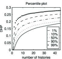
Figure 5.1: estimating $\epsilon$

The computer programs are explained and listed in appendix (E). The results described here were carried out with a system of dimension $3$, with an environment of dimension $15$ and with either medium absolute consistency or medium relative consistency (DHC). Fig. (5.1) gives the probability distribution for the DHP plotted via percentile curves as a function of the number of histories in the long time limit. For example, this graph shows that with $\epsilon\geq 0.3\approx 2/\sqrt{d}$ projections will almost certainly be consistent for any number of histories, whereas for $\epsilon\leq 0.05\approx.3/\sqrt{d}$ projections will probably only be consistent when there are two or three histories. When there are twenty histories it shows that for $98\%$ of the time the DHP will be between $0.15$ and $0.25$. Fluctuations will only occasionally ($1\%$ of the time) lie below the solid line and if $\epsilon$ has this value (for a particular number of histories) then although projections will probably occur they will occur as a result of large fluctuations from the mean. Therefore one would expect the projections to occur at widely separated times and if $\epsilon$ is changed only slightly the times generically to change completely, and indeed computer simulations show this.

The simulations described here were run for ten thousand program steps or until thirty histories had been generated. For a given set of parameters, many simulations with different Hamiltonians and initial states were carried out and were found generically to produce qualitatively the same results, though only individual simulations are described here.

(a) probability tree

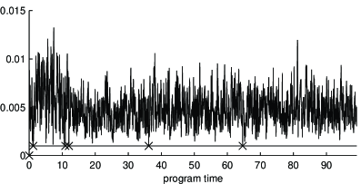
(b) consistency statistics

Figure 5.2: example

One way to look at the results of a simulation is to look at the probability tree associated with the set of histories such as fig. (5.2a). The root node on the far left represent the initial state, the terminal nodes represent the histories and the other nodes represent intermediate path-projected states. Each node has a probability and the lines linking the nodes have an associated projection operator and projection time. The projections associated with lines emanating to the right from the same node form a projective decomposition and all occur at the same time. The scaling of the axis and relative positions between the nodes is arbitrary, only the topology is relevant. For example, in fig. (5.2a) the probabilities for the histories are $0.42$, $0.25$, $0.05$, $0.02$, $0.02$, $0.01$, $0.08$ and $0.14$ — the probabilities of the terminal nodes.

Another useful interpretative aid is a graph of the consistency statistics fig. (5.2b). This graph shows the DHP for the most consistent non-trivial extension. At times where no Schmidt projections result in non-trivial histories no points are plotted, though there are no such times in fig. (5.2b). The program makes a projection when this value is $\epsilon$. The flat line indicates $\epsilon$ and the crosses indicate when projections have occurred — in this case at times $0$, $1$, $11$, $12$, $36$ and $65$ (approximately). A graph of the projection times will also be used sometimes, for example fig. (5.4b).

When any Schmidt eigenvalues are equal their eigenspaces becomes degenerate and the corresponding Schmidt projections are not uniquely defined. The reduced density matrix varies continuously in this model and it will only be degenerate for a set of times of measure zero so generically it is possible to define the Schmidt states so that they are continuous functions of $t$ for all $t$. This was not found to be necessary in the simulations.

5.3.1 Results for relative consistency

Rank one initial density matrix

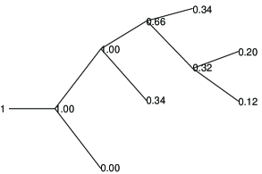
(a) probability tree

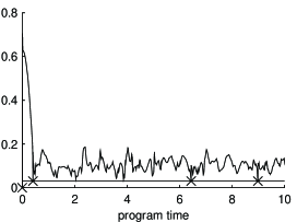
(b) consistency statistics

Figure 5.3: relative consistency, $\epsilon=0.03\approx 0.2/\sqrt{d}$

Fig. (5.3) shows the probability tree and minimum consistency statistics for a simulation with $\epsilon=0.03\approx 0.2/\sqrt{d}$ and a rank one initial density matrix. As expected there is one almost immediate trivial projection. Three more projections occur and then no more. From fig. (5.1) the probability of a projection with five histories and $\epsilon=0.03$ is less than 1% so this result is as expected. The simulation was run for longer than is shown in the figure (until $t=100$) but no further projections occurred.

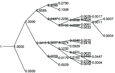
(a) probability tree

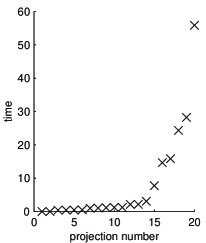
(b) projection times

Figure 5.4: relative consistency, $\epsilon=0.15\approx 1/\sqrt{d}$

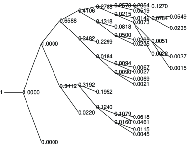
(a) probability tree

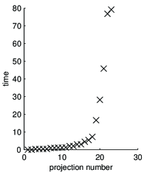
(b) projection times

Figure 5.5: relative consistency, $\epsilon=0.16\approx 1/\sqrt{d}$

Fig. (5.4) shows the probability tree and projection times for a simulation with $\epsilon=0.15\approx 1/\sqrt{d}$. Again there is the initial trivial projection but no other trivial projections occur. Projections then occurred at roughly equal equal time intervals until there were fifteen histories. The time between projections then rapidly increased. This is in accord with fig. (5.1) as the probability for a projection with fifteen histories and $\epsilon=0.15$ is around $5\%$. Projections after this time only occur for large deviation away from the mean and therefore occur extremely erratically. These later projections are extremely unlikely to vary smoothly for a range of $\epsilon$. The simulation was run until $t\approx 100$ and no further projections occurred. This simulation has produced an interesting set of histories with a complicated branching structure.

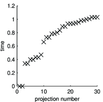
Figure 5.6: relative consistency, $\epsilon=0.3\approx 2/\sqrt{d}$

The next pair of figures fig. (5.5) shows the results of a simulation with all the parameters unchanged except for $\epsilon$ which is now $0.16$. The qualitative description is the same and the first eight or so projections are similar. After that however the two sets of histories are very different. This is the problem with the algorithm applied to this model: interesting sets of histories are produced, but they change dramatically for small changes in $\epsilon$.

From fig. (5.1) choosing $\epsilon=0.3\approx 2\sqrt{d}$ looks large enough so that projections will always be made before the background level is reached. The theoretical analysis also suggests that for such a large value of $\epsilon$ some repeated projections will occur. Indeed fig. (5.6) demonstrates that nine repeated projections occurred each giving a history of probability $\delta$.

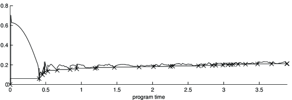
consistency statistics

Figure 5.7: relative consistency, $\epsilon$ chosen at $50\%$

An interesting alternative is to choose $\epsilon$ as a percentile from fig. (5.1), that is $\epsilon(k)\approx\epsilon(e)\log k$ where $k$ is the number of histories. Fig. (5.7) demonstrates the consistency statistics for a run with $\epsilon(k)$ chosen at the $50\%$ level. All of the probabilities except for the initial projection were non-trivial. Rather than the projections being made in regimes where the DHP fluctuates about its mean value most of the projections have been made at times when the DHP is monotonically decreasing, so that the histories are much more likely to vary continuously with $\epsilon$. Two other advantages of choosing $\epsilon$ this way are that larger sets of histories are produced, and if an algorithm is designed to produce a set of histories of a certain size choosing $\epsilon$ in this way will produce a more consistent set than choosing $\epsilon$ to be constant. However, though the results are more stable (when the percentile is changed) than for constant $\epsilon$, results from simulations show that they still change too much to single out a definite set of histories.

By looking at the consistency statistics the problem is easy to understand. Since a projection is made at the earliest possible time generically once it has been made the DHP jumps up as the most consistent projection has occurred. The consistency level then falls. While it is decreasing monotonically any change in $\epsilon$ will produce a continuous change in the time of the next projection. However, if $\epsilon$ is too far below its mean level the projection times will vary discontinuously, and all the projections afterwards will generically be completely different. Since the mean level of the DHP depends on the number of histories strongly either $\epsilon$ must be chosen sufficiently large so as to be above this or it must be chosen so as to increase with the number of histories. This is demonstrated by the first few projections as shown in fig. (5.8) — a close-up of fig. (5.7b) would also show this.

Other initial conditions

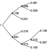
(a) probability tree

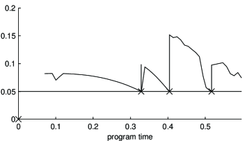
(b) consistency statistics

Figure 5.8: relative consistency, $\delta=0.02$, $\epsilon=0.05$

Simulations with a rank 2 initial state, and all other parameters remaining the same, produce the same results except that each of the initial projections is repeated producing two trivial histories with probability $\delta$. We can choose $\delta$ according to eq. (5.11) to try to prevent these projections, that is choose $\delta=O(\epsilon^{2})$. Since many of the histories we expect to generate will have probabilities smaller than this it is sensible to use a relative non-triviality criterion. The analysis leading to eq. (5.11) is only accurate to first order in $t$, therefor eq. (5.11) is only valid when $\delta$ is sufficiently small. If $\delta$ is too large the consistency level of a reprojection will start decreasing and when a reprojection eventually becomes non-trivial it will be consistent. For the example discussed there were no values of $\delta$ with $\epsilon=0.15$ that prevent an initial trivial reprojection. Fig. (5.8) demonstrates the start of a simulation with $\epsilon=0.05$ and $\delta=0.02=8\epsilon^{2}$. The graph of the consistency statistics shows the initial projection at $t=0$ and then that there are no non-trivial extensions until $t\approx 0.08$ by which time the projection is not consistent. A non-trivial projection is made at $t\approx 0.32$ and the algorithm then continues as before, with the trivial projection avoided. Because the projection has not occurred with probability $\delta$ there is a range of values for $\delta$ that do not affect the resulting histories — they are independent of $\delta$. The first three projection times will obviously vary continuously for a small range of $\epsilon$. The other projections that occurred in this simulation all occurred at much more separated times in a regime where the consistency level was not decreasing monotonically. If $\epsilon$ is chosen according to the percentile distribution in fig. (5.1) — that is $\epsilon(k)\approx\epsilon(e)\log k$ where $k$ is the number of histories — $\epsilon$ will be small enough initially to prevent any trivial projections (with an initial density matrix of rank greater than one) and will allow a full set of histories to be built up at later times.

Simulations with a full rank initial density matrix and $\epsilon=0.15$ result in a trivial repeated projection for each initial history. If $\epsilon$ is smaller ($\leq 0.07$) no trivial reprojections occur. If two initial projections are made uncorrelated with the Schmidt states then further (Schmidt) projections at $t=0$ will not generically be trivial or consistent. In both cases, after the initial projections and possible reprojections the qualitative behaviour is the same as the rank one case.

5.3.2 Results for absolute consistency

To produce interesting sets of histories from an absolute consistency criterion three effects need to be balanced against each other. If $\epsilon$ is too small the most likely projections will be those that produce very small probability histories. If $\delta/\epsilon$ is too small the likelihood of repeated projections (hence trivial histories) will be high. If $\delta$ is too large the non-triviality criterion will dominate the algorithm and only probability $\delta$ (trivial) histories will be produced. Only an absolute parameterised non-triviality criterion is considered since a relative criterion will clearly produce almost nothing except infinitesimal histories. The following results demonstrate these effects.

Rank one initial density matrix

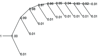
Figure 5.9: absolute consistency, $\delta=0.01$, $\epsilon=0.1$

For example if $\delta<\epsilon$ and the initial reduced density matrix has rank one the algorithm will generically produce $\lfloor 1/\delta\rfloor$ trivial histories. This is a particularly simple case of the analysis that suggests that if $\delta/\epsilon<O(1)$ repeated projections are probable. Fig. (5.9) shows an example of this from a computer simulation with $\epsilon=.1$ and $\delta=0.01$. Only the first ten projections are shown. This behaviour remains the same in the limit as $\epsilon\to 0,\delta\to 0,\delta\leq\epsilon$.

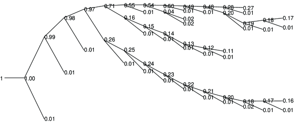
probability tree

Figure 5.10: absolute consistency, $\delta=0.01$, $\epsilon=0.02$

As the ratio $\delta/\epsilon$ increases and becomes $O(1)$ the nature of the set of histories changes. Occasionally when a reprojection becomes non-trivial it will no longer be consistent and a reprojection will not occur. A significant time may elapse before the next projection is made which will result in a non-trivial projection, which will then be followed by more trivial repeated projections. This is demonstrated in fig. (5.10) where $\epsilon=0.02$ and $\delta=0.01$. Though this is an interesting set of histories this range of parameter values does not give a theory with predictive power since simulations show that the results vary enormously for small changes in $\epsilon$ and $\delta$.

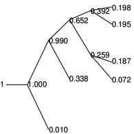
(a) probability tree

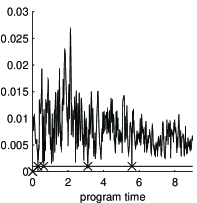
(b) consistency statistics

Figure 5.11: absolute consistency, $\delta=0.01$, $\epsilon=0.001$

As $\delta/\epsilon$ increases past $1$ the number of histories made with probability $\delta$ decreases to just the initial projection. Fig. (5.11) shows that this range of parameter values produces interesting histories but the projections are occuring at times when the consistency level is fluctuating randomly about the mean and so will be unstable to small changes in $\epsilon$.

Other initial conditions

Choosing larger rank initial reduced density matrices or initial projections does not qualitatively change the analysis. The only difference is that for $\delta>\epsilon$ and $\epsilon$ sufficiently small no trivial projections will be made.

5.4 Conclusions

The algorithm produces sets of histories with a complicated branching structure and with many non-trivial projections for a range of parameter values. Algorithms using the DHC produce results that are essentially the same for a wide range of $\delta$ (the non-triviality parameter) including the limit $\delta\to 0$. However, the algorithm does not make useful predictions when applied to this model since the results vary erratically with $\epsilon$ and there is no special choice of $\epsilon$ singled out. Choosing $\epsilon$ as a function of the number of histories according to fig. (5.1) produces the least unstable sets of histories and the largest sets of non-trivial histories, but even in this case the algorithm does not single out a definite set.

The algorithm is less effective when used with an absolute consistency criterion: in this case the predictions of the algorithm also vary erratically with $\delta$ and the resulting sets of histories include fewer non-trivial histories.

The results of the simulations agree well with the theoretical analysis of section (5.2) and demonstrate features of the algorithm that will also apply to other models — such as the analysis of repeated projections. They also demonstrate some of the difficulties that an algorithm must overcome. These problems can be related to the discussion of recoherence in section (4.4). The algorithm will only produce stable results (with respect to $\epsilon$) if the projections occur when the off-diagonal terms of the decoherence matrix are monotonically decreasing. This behaviour is only likely in a system like this for times small compared to the recurrence time of the system and when the number of histories is small compared to the size of the environment Hilbert space. The results of the model do show stability for the first few projections and if much larger spaces were used this behaviour would be expected for a larger number of histories. In particular as the size of the environment goes to infinity it is plausible that the algorithm applied to this model will produce a large, stable, non-trivial set of histories.

In retrospect it was ambitious to hope that an algorithm applied to this model would produce large sets of stable histories. A random model like this, with such a small environment, will generically only decohere a few histories (see also [151, 152].)

Chapter 6 Maximum information

6.1 Introduction

Chapters 4 and 5 have shown some of the difficulties in formulating a successful set selection algorithm. Indeed section 4.4 shows that in many systems no algorithm that constructs sets by proceeding forwards in time will produce the correct physical set. An algorithm must consider the entire time evolution of a system if it is always to overcome this problem. This chapter introduces a new algorithm that is global with respect to time: it considers the class of all consistent sets of histories formed from Schmidt projections and selects from among them the one with the greatest Shannon information [165].

Information is a term often used in the study of quantum mechanics and is used in many different senses. Hartle [125] considers the missing information of a set of histories in a generalised spacetime quantum mechanics — he defines the missing information S of a set of histories $\mathcal{S}$ with initial density matrix $\rho$ as

$$S(\mathcal{S},\rho)=\max_{\rho^{\prime}\in\{D(\mathcal{S},\rho^{\prime})=D(\mathcal{S},\rho)\}}E(\rho^{\prime})\,,$$ (6.1)

where $D(\mathcal{S},\rho)$ is the decoherence matrix for the set of histories $\mathcal{S}$ with initial density matrix $\rho$. Throughout this chapter $E$ will denote the Shannon information of a set of probabilities or, in the case of a positive definite Hermitian matrix, the Shannon information of its eigenvalues. So, for example, $E(\rho^{\prime})=-\mbox{Tr}\rho^{\prime}\log\rho^{\prime}$ and

$$E(\mathcal{S},\rho)=\sum_{\alpha\in\mathcal{S}}-D_{\alpha\alpha}\log D_{\alpha\alpha}\,,$$ (6.2)

where $\{D_{\alpha\alpha}\}$ are the diagonal elements of the decoherence matrix $D(\mathcal{S},\rho)$. Note that if a set of histories $\mathcal{S}$ is medium consistent then $E({\mathcal{S}},\rho)=E[D(\mathcal{S},\rho)]$: generically this is not true for weak consistency criteria.

$S(\mathcal{S},\rho)$ is the information content of a maximum-entropy [166] estimation of the initial density matrix given the set of histories and their probabilities— it quantifies what can be inferred about the initial density matrix using the set of histories and their probabilities. Hartle goes on to define

$$S(\mathcal{G},\rho)=\min_{\mathcal{S}\in\mathcal{G}}S(\mathcal{S},\rho),$$ (6.3)

where $\mathcal{G}$ is some class of consistent sets of histories. Computing $S(\mathcal{G},\rho)$ for different classes enables one to understand different ways information about a quantum system can be obtained. For example Hartle suggests comparing whether the same information is available using homogeneous [93] histories instead of the more general inhomogeneous histories. When $\mathcal{G}$ is the class of all consistent sets he calls $S(\mathcal{G},\rho)$ the complete information.

Eq. (6.3) could be used as the basis for a set selection algorithm by specifying some class of sets of histories $\mathcal{G}$ and selecting a set of histories that produces the minimum in eq. (6.3). This does not work for general classes, since if the class contains sets of histories which include projections onto the eigenspaces of $\rho$ (in non-relativistic quantum mechanics) these projections completely specify $\rho$, so a rather uninteresting set of histories is selected. However, if the initial state is pure and a Schmidt class (a class of sets of histories formed from Schmidt projections) is used it will not generically contain a set of histories that includes a rank one projection onto the initial state, hence the set of histories selected by eq. (6.3) might not be trivial. For instance the set of histories consisting of projections $P\otimes I$ and $\overline{P}\otimes I$, where $P$ is the projection onto the non-zero system Schmidt eigenspaces, has missing information $\log\mbox{rank}(P\otimes I)$. It might be considered unnatural to assume a pure initial state and then make a maximum entropy calculation over density matrices of other ranks; however, this idea has a more serious flaw. The aim of set selection algorithms is to make statements concerning physical events, not merely to supply initial conditions. This algorithm only searches for a set of histories that best specifies the initial conditions and there is no reason to expect it to produce sets that do more than describe the initial conditions.

Isham and Linden [167] very recently proposed a different version of missing information, which they call information-entropy, that is simpler and does not use ideas of maximum entropy.

$$S^{\prime}(\mathcal{S},\rho)=-\sum_{\alpha\in\mathcal{S}}D_{\alpha\alpha}\log\frac{D_{\alpha\alpha}}{\mbox{dim}^{2}(\alpha)}\,,$$ (6.4)

where $\mbox{dim}(\alpha)=\mbox{Tr}(C_{\alpha})$ when $C_{\alpha}$ is considered as an operator in the $n$-fold tensor product space [99, 168] of $\mathcal{H}$. For example if the history $\alpha$ is defined by consecutive projections $\{P_{k},k=1,\ldots,n\}$ then $\mbox{dim}(\alpha)=\mbox{Tr}(P_{1}\otimes\cdots\otimes P_{n})=\mbox{rank}(P_{1})\times\cdots\times\mbox{rank}(P_{n})$. Like Hartle’s missing information, $S^{\prime}$ decreases under a refinement of $\mathcal{S}$ and

$$S^{\prime}(\mathcal{S},\rho)\geq-\mbox{Tr $\rho\log\rho$}\,.$$ (6.5)

Isham and Linden show for some examples that

$$\min_{\mathcal{S}\in\mathcal{G}}S^{\prime}(\mathcal{S},\rho)=-\mbox{Tr $\rho\log\rho$}$$ (6.6)

and conjecture that the bound is attained in general. These are interesting results and suggest a useful definition of information — especially in complicated spacetimes. Isham and Linden also suggest that information-entropy might help in the development of a set selection criterion. Although they have not yet made a definite proposal, they suggest that perhaps the minimisation should be carried out with respect to a system–environment split. Clearly some restriction on the class of sets used is necessary since bound (6.5) contains no mention of the Hamiltonian or time evolution of the system — simply minimising information-entropy is unlikely to produce a good set selection algorithm, since the sets of histories that describes experimental situations are much more than a description of the initial conditions.

Gell-Mann and Hartle discuss similar ideas in detail in ref. [95]. They introduce a measure, which they call total information or augmented entropy, $\Sigma$ that combines algorithmic information (see for example ref. [169]), entropy-information and coarse graining. This is an attempt to provide a quantitative measure of quasiclassicality. They show that minimising $\Sigma$ does not provide a useful set selection algorithm — the results are trivial, histories are selected that consist of nothing but projections onto the initial state — but they suggest augmenting the minimisation with a stronger consistency criterion,

$$\langle\alpha|M^{\dagger}_{\alpha}M_{\beta}|\beta\rangle=p_{\alpha}\delta_{\alpha\beta}\mbox{~{}$\forall\alpha\neq\beta$, $M_{\alpha}\in\mathcal{M}_{\alpha}$ and $M_{\beta}\in\mathcal{M}_{\beta}$,}$$ (6.7)

where $\mathcal{M}_{\alpha}$ and $\mathcal{M}_{\beta}$ are sets of operators. This is an interesting idea. So far however, Gell-Mann and Hartle have not proposed a definite algorithm for choosing the $\mathcal{M}_{\alpha}$. Without a concrete scheme for choosing the sets $\mathcal{M}_{\alpha}$ the set selection problem of course becomes the problem of selecting $\mathcal{M}_{\alpha}$. Gell-Mann and Hartle proposal also has the previously mentioned disadvantage of appearing to favour set of histories that only provide a description of the initial state and say nothing about the evolution.

The approach we present here starts with a precisely defined class of quasiclassical sets of histories (formed from Schmidt projections) and picks the set of histories from this class with the largest information.

6.2 Algorithm

Let $\mathcal{G}(\mathcal{H},U,|\psi\rangle)$ be the class of all sets of non-trivial, exactly consistent, branch-dependent histories formed from Schmidt projection operators, where $\mathcal{H}=\mathcal{H}_{1}\otimes\mathcal{H}_{2}$ is a finite Hilbert space, $U(t)$ a time evolution operator and $|\psi\rangle$ the initial state. Note that in this section the set of histories includes the initial state. The algorithm selects the set $\mathcal{S}\in\mathcal{G}$ with the greatest Shannon information. That is

$$\max_{\mathcal{S}\in\mathcal{G}}E(\mathcal{S})=\max_{\mathcal{S}\in{\mathcal{G}}}\sum_{\alpha\in\mathcal{S}}-p_{\alpha}\log p_{\alpha},$$ (6.8)

where $p_{\alpha}$ is the probability of history $\alpha$. The class $\mathcal{G}$ could be chosen differently by using any of the consistency or non-triviality criteria from chapter 3. Another variant uses sets of histories formed by Schmidt projections onto the system eigenspaces of the individual path-projected-states ($U(t)C_{\alpha}|\psi\rangle$), not the total state (see sec. 4.6), so that the choice of projections is branch-dependent as well as the choice of projection times. This is likely to be necessary in general to produce realistic sets.

When the initial state is pure, in a Hilbert space of dimension $d$ ($=d_{1}d_{2}$) there can only be $d$ non-trivial, exactly consistent histories. In realistic examples approximate consistency may have to be considered. To ensure the algorithm is well defined it is important that the number of possible history vectors in a set is finite, which will only be true if we use a parameterised non-triviality criterion or we use a consistency criterion, such as the DHC, that can only be satisfied by a finite number of history vectors [2]. This is a natural requirement for any set of histories in a finite Hilbert space since the exactly consistent sets are finite.

Eq. (6.8) selects an equivalence class of sets of histories that all have the maximum information. The equivalence relation is defined by $\mathcal{S}_{1}\sim\mathcal{S}_{2}$ if $E(\mathcal{S}_{1})=E(\mathcal{S}_{2})$; that is, sets of histories are equivalent if they have the same information. Sufficient conditions for eq. (6.8) to be well defined are that $\mathcal{G}/\kern-3.50006pt\sim$ is closed and that $E(\mathcal{S})$ is bounded. $\mathcal{G}$ itself is not closed, but the only limit sets of histories it does not include are those containing zero probability histories, and since zero probability histories contribute zero information these limit sets are equivalent to sets which are in $\mathcal{G}$, hence $\mathcal{G}/\kern-3.50006pt\sim$ is closed. Moreover these limit sets are also physically equivalent to some of the sets that they are information-equivalent to, since they only differ by zero probability histories — excluding the limit sets does not change anything physical. The information of any set of histories in $\mathcal{G}$ is bounded, since the number of histories in any set of histories in $\mathcal{G}$ is bounded and the information of a set of $n$ probabilities is bounded by $\log n$. Conditions sufficient to ensure uniqueness are much more complicated. Probably the best that one can hope for in many situations is that a class of physically equivalent sets is selected.

First we describe some useful properties of this algorithm and then we apply it to a simple model.

6.2.1 Completeness

The set of histories selected by the algorithm cannot be extended (except trivially) because any non-trivial extension increases the information content. To see this consider the set of histories ${\mathcal{S}}$ and an extension $\mathcal{S}^{\prime}$. The probabilities for the new histories can be written in the form $p_{\alpha}q^{(\alpha)}_{\beta}$ where $\sum_{\beta}q^{(\alpha)}_{\beta}=1$ for all $\alpha$. The information of the new set is

$$E(\mathcal{S}^{\prime})=-\sum_{\alpha}\sum_{\beta}p_{\alpha}q^{(\alpha)}_{\beta}\log p_{\alpha}q^{(\alpha)}_{\beta}=E(\mathcal{S})+\sum_{\alpha}p_{\alpha}E(q^{(\alpha)}_{\beta}),$$ (6.9)

which is strictly greater than $E(\mathcal{S})$ whenever the extension results in at least one non-zero probability.

6.2.2 Additivity

A set of branch-dependent histories has a probability tree structure, where each history $\alpha$ refers to a terminal node of the tree and the unique path from that node to the root node. The nodes themselves are associated with projection operators and path projected states. Define $\mathcal{S}_{\alpha k}$ to be the set of all histories extending from the $k^{\mbox{\scriptsize th}}$ node of history $\alpha$, normalised so that the total probability is one. This is a set of histories in its own right which will be consistent if the entire set of histories is consistent. Consider a simple example where the first projection produces two histories with probabilities $p$ and $q$ and the subtrees from these nodes are ${\mathcal{S}}_{p}$ and $\mathcal{S}_{q}$. The information for the set of histories can then be written,

$$E(\mathcal{S})=E(\{p,q\})+pE(\mathcal{S}_{p})+qE(\mathcal{S}_{q}).$$ (6.10)

This formula is easy to generalise. Each subtree must have maximum information subject to the constraint that the history vectors span a space orthogonal to the other history states. That is, a global maximum must also be a local maximum in each degree of freedom and the subtrees are the degrees of freedom.

6.2.3 Large sets

One of the problems with the algorithms in chapter 3 is their tendency to make projections too early so that they prevent projections at later times. Other problems also arise with algorithms that produce histories with zero or small probabilities. The maximum-information algorithm will not have these problems, since any projection that prevents later extensions is unlikely to be selected, histories with zero probability will never be selected (since they contribute no information), and histories with small probabilities are also unlikely to be selected. Therefore the algorithm is much more likely to produce large complicated sets of histories than previous algorithms.

6.2.4 Stability

Another problem with the algorithms in chapter 3 was demonstrated in chapter 5: the predictions are unstable to perturbations of the Hamiltonian or initial state, and the predictions vary erratically with the choice of the approximate consistency parameter. It is difficult to prove any general results about stability for this algorithm, but it seems much more likely to produce stable predictions for the following reasons. There is no reason why any projections should be made that exactly satisfy the approximate consistency criterion, whereas in an earliest time algorithm this is the generic result. For example, if a set is predicted that is exactly consistent the same set could still be predicted for any reasonably small $\epsilon$. There are also unlikely to be complications caused by trivial histories, since these contribute little information and are not likely to be selected by the algorithm. The sets of histories described by the Schmidt projections generically will vary continuously with sufficiently small changes in the initial state and Hamiltonian. Therefore we expect generically that for a range of approximate consistency parameters the selected set will also vary continuously. This is a generic result for continuous optimisation problems: they are stable for small perturbations.

6.3 The spin model

A set of histories that maximises information must be complete, therefore all histories must consist of projections at times $\{1,\ldots,k-1,t,k:t\in(k-1,k)\}$. First we show that $k$ must be the same for all histories (that is, the set is branch independent), then we calculate $k$.

The information content of two subtrees rooted at the same point only depends on the projection times within each one. Either the two subtrees have the same information, in which case their projection times must be the same, or one has more, but since the projection times used in the subtree with greater information will also be consistent if used in the subtree with less information these projection times can be used instead. Therefore in the set with maximum information all the subtree must have the same projection times, thus all the histories must have the same projection times — the maximal set is branch independent.

Let the projection times be $\{1,\ldots,k-1,t,k:t\in(k-1,k)\}$. Then from eq. (4.53) and eq. (6.9) the information content of this set is

$$f[N_{k}(\theta_{k}(t))]+f[({\bf u}_{k}.{\bf u}_{k-1})N_{k}^{-1}(\theta_{k}(t))]+\sum_{k>j>0}f({\bf u}_{j-1}.{\bf u}_{j})$$ (6.11)

where

$$f(x)=-\frac{1+x}{2}\log\frac{1+x}{2}-\frac{1-x}{2}\log\frac{1-x}{2}.$$ (6.12)

Maximising eq. (6.11) with respect to $t$ yields

$$E(\mathcal{S}_{k})=E_{k}=2f(|{\bf u}_{k}.{\bf u}_{k-1}|^{1/2})+\sum_{k>j>0}f({\bf u}_{j-1}.{\bf u}_{j}),$$ (6.13)

where $\mathcal{S}_{k}$ is the branch independent set consisting of projections at times $\{1,\ldots,k-1,t_{k},k\}$. This is usually maximised by $k=n$ but depending on the relationships between the ${\bf u}_{j}$ any value of $k$ may be possible. For example, consider ${\bf u}_{j-1}.{\bf u}_{j}=1-\epsilon$ for all $j\neq k$ and ${\bf u}_{k-1}.{\bf u}_{k}=\epsilon$ and $\epsilon$ is small.

$$E_{m}=\left\{\begin{array}[]{lr}O(\epsilon\log\epsilon),&\mbox{for $m<k$},\\ 2\log 2+O(\epsilon\log\epsilon),&\mbox{for $m=k$},\\ \log 2+O(\epsilon\log\epsilon)&\mbox{for $m>k$},\end{array}\right.$$ (6.14)

which for small $\epsilon$ is maximised by $E_{k}$.

The precise relationship between the $\{{\bf u}_{j}\}$ that ensure $E_{n}>E_{k}$ for all $k<n$ is complicated in detail, but simple qualitatively. Roughly speaking, $E_{n}<E_{k}$ only if $|{\bf u}_{j-1}.{\bf u}_{j}|\gg|{\bf u}_{k-1}.{\bf u}_{k}|$ for all $j>k$, that is all the measurement directions must be approximately parallel after the $k^{\mbox{\scriptsize th}}$. Monte Carlo integration over $\{{\bf u}_{i}\}$ (with the $SO(3)$ invariant measure) shows that for $n=3$ set $\mathcal{S}_{n}$ is selected $85.7\%$ of the time, for $n=4$ it is selected $84.3\%$ of the time, and for all $n>4$ it is selected $84.2\%$ of the time. When the vectors are approximately parallel, that is $|{\bf u}_{j-1}.{\bf u}_{j}|=1-O(\epsilon)$, set $S_{n}$ is selected with probability $1-O(\epsilon)$. If however all the measurement spins are approximately parallel ($|\mathbf{u}_{j-1}.\mathbf{u}_{j}|>1-\epsilon$, and $-n\epsilon\log\epsilon<4\log 2$) then for some orientations of the initial system spin (${\bf v}={\bf u}_{0}$) $E_{1}>E_{k}$ for all $E_{k}$ so set $\mathcal{S}_{1}$ is selected. That is, the maximal set consists only of a projection during the first interaction and at the end of the first interaction.

Though the results of the algorithm may seem counterintuitive the following discussion shows why this is not a problem.

First consider the case when the system is genuinely closed. All the projections before the last interaction are natural. It is only the projections during the last interaction, which occur when the set of histories is nearly complete, that are unnatural. Our intuition about the system and the result we believe to be correct relies on the experiment being imbedded in a larger system in which the sets of histories considered are always far from complete.

Second consider the case where the system is approximately closed. Then the sets $\mathcal{S}_{k}$ should describe the first projections of a maximum-information solution in a larger Hilbert space. For reasons explained below, no non-trivial projections onto the system space will result in consistent extensions of the sets $\mathcal{S}_{k}$, even if the system interacts with new degrees of freedom in the environment. This shows that though it is a maximum-information set for a subsystem, it is unlikely to be part of the maximum-information set for the entire system. The set most likely to be part of the maximum-information set is the natural set, the set that consists of projections only at the end of each interaction.

The set of normalised histories (in the Schrödinger picture at time $k$, that is the path-projected states) is

$$\mathcal{S}_{k}=\{|\alpha_{0}{\bf v}_{k}\rangle\otimes|\alpha_{1}(\uparrow),\ldots,\alpha_{k-1}(\uparrow),\alpha_{k}(\rightarrow),\uparrow_{k+1},\ldots,\uparrow_{n}\rangle\forall\alpha\in Z_{2}^{k+1}\},$$ (6.15)

where $\alpha$ is a string of $2^{k+1}$ plusses and minuses, $+(\uparrow)=\uparrow$, $-(\uparrow)=|\downarrow\rangle$ and $\pm(\rightarrow)$ are orthogonal vectors depending on $\mathbf{u}_{k-1}$ and $\mathbf{u}_{k}$. This set of histories cannot be non-trivially extended with Schmidt projections (see sec. 4.2). The reason for this is clear. Consider two of the histories $|{\bf\pm v}_{k}\rangle\otimes|e\rangle$ where $|e\rangle$ is the environment state. These histories are only orthogonal because of the orthogonality of the system part of the states. There can be no future non-trivial extensions unless there is an exact degeneracy, because consistency terms between these two histories will contain terms like $|\langle{\bf v}|P({\bf w})|{\bf v}\rangle|=\sqrt{1/2(1+{\bf v}.{\bf w})}$, which is only zero when $\mathbf{w}=-\mathbf{v}$. In contrast if projections are only made at the end of interactions all the histories are orthogonal in the environment Hilbert space of the finished interactions. Unless these interactions are “undone” these histories will always remain orthogonal and cannot interfere. This argument suggests that the true maximum-information set for the total Hilbert space starts of with projections at the end of every interaction but at no interior times.

This suggests that an algorithm designed to produce a maximum-information set for a subsystem could be constructed by requiring that all the histories in a set were orthogonal in the environment space, that is the reduced density matrices in the environment Hilbert space for each history are orthogonal. This is related to the strong consistency criterion eq. (6.7) when the sets $\mathcal{M}_{\alpha}$ are all chosen to be the set $\{P\otimes I:\forall P^{2}=P\,,P^{\dagger}=P\}$.

6.4 Other algorithms

Let $\mathcal{G}(\mathcal{H},U,|\psi\rangle)$ be the class of all sets of non-trivial, exactly consistent, branch-dependent histories formed from Schmidt projection operators in the spin model. Consider an algorithm that selects the set in $\mathcal{G}$ that minimises Isham and Linden’s information-entropy (6.4). Due to the special symmetries of the spin model the selected set will be branch independent — the argument at the start of section (6.3) is valid.

Consider the set of projections at $m$ times, so that the dimension of each history is $(d/2)^{m}$, where $d$ is the dimension of the total Hilbert space. Information-entropy for this set is

$$S^{\prime}=-\sum_{\alpha\in\mathcal{S}}p_{\alpha}\log\frac{p_{\alpha}}{(d/2)^{2m}}=2m\log(d/2)-\sum_{\alpha\in\mathcal{S}}p_{\alpha}\log p_{\alpha}\,.$$ (6.16)

This is minimised for $m=0$ — the selected set consists of no projections at all — which is not a natural set. The problem with directly using minimum-information-entropy as a set selection criterion is clear; the information-entropy will consist of two terms, one roughly proportional to the number of projection times and another that is the Shannon information of the probabilities, both of which are minimised by the set with the fewest histories.

Isham and Linden show that information-entropy decreases when the set is refined by replacing a projective decomposition by a finer one. However, if the set is extended by adding projections at a new time then the information-entropy increases, and since the proposal is to minimise information-entropy this algorithm will always select the set of histories in the class with the fewest histories. There are two obvious approaches to this difficulty, which are largely equivalent. One could extend (with the identity projection) all the sets of histories in the class so that projections occur at the same times in all sets. Adding a projection would then be a refinement of the identity and the information-entropy would decrease. However, it is not all obvious that this is well defined in general, though there are no problems in this example. When it is well defined it yields the same results as the more natural modification of using the normalised dimension, $\widehat{\mbox{dim}}$, in the formula (6.4) information-entropy. For a homogenous history

$$\widehat{\mbox{dim}}\ \alpha=\frac{\mbox{dim }P_{\alpha_{1}}\times\cdots\times\mbox{dim }P_{\alpha_{m}}}{\mbox{dim }I\times\cdots\times\mbox{dim }I}=(\mbox{dim }\alpha)/d^{m}\,,$$ (6.17)

where $d=\mbox{dim }I$ the dimension of the Hilbert space. With this definition information-entropy decreases for all refinements and extensions.

The information-entropy with normalised dimension is

$$S^{\prime\prime}=-2m\log 2-\sum_{\alpha}p_{\alpha}\log p_{\alpha}\,.$$ (6.18)

Using the notation of the previous section this can be written

$$S^{\prime\prime}=-\sum_{m>k>0}[2\log 2-f(\alpha_{k})]\,,$$ (6.19)

where the $\alpha_{k}$ depend on the projection times and vary between $-1$ and $1$. Since $f(x)\leq\log 2$ each term in the sum is always negative so the minimum occurs for $m=n+1$, and the selected set consists of projections at the end of every interaction and a projection either at the end or the beginning of the last interaction — the algorithm has selected a natural set. The revised (using normalised dimension) minimum-information-entropy algorithm selects a set with as many projections as possible, and among these sets it selects the set whose probabilities have the lowest Shannon information. Though using $S^{\prime\prime}$ has worked well here this approach would probably not be successful in general as the algorithm will tend towards making a large number of repeated projections and these will be greatly favoured over more complicated sets. The set of normalised dimensions $\{\hat{d}_{\alpha}\}$ has an interpretation as a set of probabilities. Perhaps a more natural selection scheme would be to minimise the difference in Shannon information between the $\{\hat{d}_{\alpha}\}$ and the $\{p_{\alpha}\}$. An approach like this may work in particular situations but all the suggestions in this section (6.4) appear ad hoc and unsuitable as a part of a fundamental theory.

6.5 Conclusions

This chapter defines a precise algorithm for making probabilistic predictions for closed quantum systems. The algorithm considers the class of all non-trivial, exactly consistent, branch-dependent sets of histories defined by Schmidt projections with respect to a fixed split of the Hilbert space and selects from among them the set with the largest Shannon information. The algorithm avoids many of the problems of the algorithms we considered earlier in chapter 3. Because it considers the entire time evolution of a system – roughly speaking it is global in time, whereas the algorithms in chapter 3 are local — it does not make unphysical projections in systems where recoherence occurs and it produces complete sets of histories that describe the correlations between the system and the environment. Trivial and very small probability histories, which cause problems for some of the algorithms considered earlier by preventing later physical projections, are unlikely to be selected since they contribute little information. The algorithm is also likely to be stable under perturbations in the initial conditions, the Hamiltonian and the parameters, since it involves maximising a continuous function.

Section (6.3) has shown that the algorithm selects a natural set for a simple spin model. It would be interesting to test out the algorithm on more realistic examples; however, it seems difficult to apply the algorithm directly, because of the large size and complicated nature of $\mathcal{G}$. Analytic calculations are only possible when the system is very simple and in more realistic examples computer simulations will be necessary. However, it should be possible at least to get some insight into the algorithm’s predictions by maximising subject to constraints, that is by considering a more computationally tractable subset of $\mathcal{G}$. For example, we could choose a time interval $T$ that is greater than the time of individual interactions (within the particular system) and larger than any timescale over which recoherence occurs. This would be used as a moving time-window over which to perform the maximisation. The earliest projection within each time-window would be selected and the next time-window would commence from that time. Such algorithms should select the same set as a global algorithm if $T$ is large enough, and are also independently interesting.

Because the algorithm predicts the probabilities for events and the set of possible events the algorithm is falsifiable. For example the algorithm is wrong if it selects any sets that do not agree with our experiences. The algorithm can also be applied to situations where we have no experience of what the natural sets of histories are: for example, a (finite) closed system of electrons and photons — and perhaps ultimately could be applied to theories of quantum cosmology. The algorithm, like other tentative proposals in the literature [167, 95], has not yet been tested in a wide range of realistic physical examples: further investigations would clearly be worthwhile.

Appendix A Probability distributions

The notation $1_{\mathbf{x}\in A}$ is used to denote an indicator function in this dissertation, that is

$$1_{\mathbf{x}\in A}=\left\{\begin{array}[c]{lr}1&\mbox{if $\mathbf{x}\in A$}\\ 0&\mbox{if $\mathbf{x}\not\in A$}\end{array}\right.\,.$$ (A.1)

A.1 Sum of $k$ components of a random vector in $S^{d-1}$

Let $A$ be the random variable

$$A=\sum_{k\geq i\geq 1}X_{i}^{2}\,,$$ (A.2)

where $X_{i}$ are the $d$ components of a random vector uniformly distributed in $S^{d-1}$. That is, $A$ is the sum of the first $k$ components of a random unit vector in $R^{d}$. $\mathbf{X}$ can be written $\mathbf{X}=\mathbf{Y}/|\mathbf{Y}|$, where $Y_{i}$ are identical, independent, mean zero, normal random variables, since the probability density function is proportional to $e^{-|\mathbf{Y}|^{2}}$. Then

$$P(A<\lambda)=P\left(\frac{\sum_{k\geq i\geq 1}Y_{i}^{2}}{\sum_{d\geq i\geq 1}Y_{i}^{2}}<\lambda\right)=P\left(\frac{\chi^{2}_{k}}{\chi^{2}_{k}+\chi^{2}_{d-k}}<\lambda\right),$$ (A.3)

where $\chi^{2}_{k}$ and $\chi^{2}_{d-k}$ are independent, Chi-squared random variable with $k$ and $d-k$ degrees of freedom respectively. This ratio of Chi-squared variable is a beta variable with distribution function

$$B[\lambda;k/2,(d-k)/2]=\frac{\Gamma(d/2)}{\Gamma(k/2)\Gamma[(d-k)/2]}\int_{0}^{\lambda}dx\,x^{k/2-1}(1-x)^{(d-k)/2-1},$$ (A.4)

which has mean $k/d$ and variance $\frac{k(d-k)}{d^{2}(d/2+1)}$. A complex unit vector $\mathbf{Z}\in CS^{d-1}$ can be regarded as a real vector in $S^{2d-1}$ so

$$P\left(\sum_{k\geq i\geq 1}|Z_{i}|^{2}<\lambda\right)=B[\lambda;2k/2,(2d-2k)/2]=B(\lambda;k,d-k).$$ (A.5)

A.2 Maximum of $k$ components of a random vector in $S^{d-1}$

Let $A$ be the random variable

$$A=\max_{k\geq i\geq 1}X_{i}^{2}\,,$$ (A.6)

where $X_{i}$ are the $d$ components of a random vector uniformly distributed in $S^{d-1}$ and $f(\lambda)=P(A<\lambda)$. The probability density function for $\mathbf{X}$ is $N_{d}\,\delta(1-|\mathbf{X}|^{2})$, where $N_{d}=\Gamma(d/2)/(2\pi^{d/2})$. Therefore

$$f(\lambda)=N_{d}\int d\mathbf{x}\,\delta(1-|\mathbf{x}|^{2})\prod_{k\geq i\geq 1}1_{x_{i}^{2}<\lambda}\,.$$ (A.7)

After changing variables $\mathbf{x}\to\mathbf{x}/\sqrt{r}$ and $\mathbf{\lambda}\to\mathbf{\lambda}/r$ eq. (A.7) is

$$f(\mathbf{\lambda}/r)=r^{-d/2}N_{d}\int d\mathbf{x}\,\delta(1-|\mathbf{x}|^{2}/r)\prod_{k\geq i\geq 1}1_{x_{i}^{2}<\lambda}\,.$$ (A.8)

Multiply both sides by $r^{n/2-1}$ and integrate with respect to $r$ from $0$ to $\infty$.

$$\int_{0}^{\infty}dr\,r^{n/2-1}e^{-r}f(\mathbf{\lambda}/r)=N_{d}\int d\mathbf{x}\,e^{-|\mathbf{x}|^{2}}\prod_{k\geq i\geq 1}1_{x_{i}^{2}<\lambda}=\Gamma(d/2)\prod_{k\geq i\geq 1}\mbox{erf}(\sqrt{\lambda})\,.$$ (A.9)

Rescale $\mathbf{\lambda}\to p\mathbf{\lambda}$ and $r\to rp$.

$$p^{d/2}\int_{0}^{\infty}dr\,r^{d/2-1}e^{-rp}f(\mathbf{\lambda}/r)=\Gamma(d/2)\prod_{k\geq i\geq 1}\mbox{erf}(\sqrt{p\lambda})\,.$$ (A.10)

The l.h.s. is a Laplace transform of the function $r^{d/2-1}f(\mathbf{\lambda}/r)$ with respect to the variable $p$, so using the Laplace inversion theorem

$$r^{n/2-1}f(\mathbf{\lambda}/r)=\frac{\Gamma(d/2)}{2\pi i}\int_{\gamma-i\infty}^{\gamma+i\infty}dp\,e^{rp}p^{-d/2}\prod_{k\geq i\geq 1}\mbox{erf}(\sqrt{\lambda p})\,.$$ (A.11)

Finally let $r=1$

$$f(\mathbf{\lambda})=\frac{\Gamma(d/2)}{2\pi i}\int_{\gamma-i\infty}^{\gamma+i\infty}dp\,e^{p}p^{-d/2}\prod_{k\geq i\geq 1}\mbox{erf}(\sqrt{\lambda p})\,.$$ (A.12)

This integral is very complicated. However, when $d\lambda=O(1)$ and $k^{2}/d=o(1)$ we can perform an asymptotic expansion in $d$ using the method of steepest descents. The saddle point is at $p=\sqrt{d/2}$ and the steepest descent contour is $p(x)=-W(-e^{x^{2}-1})$, where $W$ is Lambert’s W function. The first two terms are

$$\mbox{erf}^{k}(\sqrt{d\lambda/2})\left[1+\frac{k\sqrt{\lambda}(d\lambda-3)e^{-d\lambda/2}}{2\sqrt{2\pi d}\,\mbox{erf}(\sqrt{d\lambda/2})}-\frac{k(k-1)\lambda e^{-d\lambda}}{2\pi\,\mbox{erf}^{2}(\sqrt{d\lambda/2})}+O(1/d^{2})\right],$$ (A.13)

which equals $\mbox{erf}^{k}(\sqrt{d\lambda/2})[1+O(k^{2}/d)]$. This shows that if we are looking at fewer than $\sqrt{d}$ components of a unit vector we can accurately approximate the distribution by considering $k$ independent normal variable with variance $1/d$ for $\lambda<1/k$.

The complex case is more straightforward. Let $A^{\prime}$ be the random variable

$$A^{\prime}=\max_{k\geq i\geq 1}|Z_{i}|^{2}\,,$$ (A.14)

where $Z_{i}$ are the $d$ components of a random vector uniformly distributed in $CS^{d-1}$ and $f^{\prime}(\lambda)=P(A^{\prime}<\lambda)$. The same method can be used in the complex case to get

$$f^{\prime}(\mathbf{\lambda})=\frac{\Gamma(d)}{2\pi i}\int_{\gamma-i\infty}^{\gamma+i\infty}dp\,e^{p}p^{-d}(1-e^{-\lambda p})^{k}\,,$$ (A.15)

and then

$$f_{k}^{\prime}(\lambda) = \frac{\Gamma(d)}{2\pi i}\sum_{m}(-1)^{m}{k\choose m}\int_{\gamma-i\infty}^{\gamma+i\infty}dp\,1_{m\lambda<1}e^{p(1-m\lambda)}p^{-d}$$ (A.16)

$$= \sum_{m}(-1)^{m}{k\choose m}(1-m\lambda)^{d-1}1_{m\lambda<1}$$ (A.17)

If $d\lambda^{2}k^{2}=o(1)$ then eq. (A.16) becomes

$$\sum(-1)^{m}{k\choose m}e^{-dm\lambda+O(m^{2}/d)}=(1-e^{-d\lambda+o(1)})^{k}]\,.$$ (A.18)

Note that the form of the answer is essentially the same in the real and complex cases.

A.3 Two orthonormal vectors in $S^{d-1}$

Consider two orthonormal random vectors $\mathbf{X}$ and $\mathbf{Y}$ in $S^{d-1}$. The probability density function is proportional to $\delta(1-\mathbf{x}^{2})\delta(1-\mathbf{y}^{2})\delta(\mathbf{x}.\mathbf{y})$ so

$$P(\mathbf{X}\in A,\mathbf{Y}\in B)=\int d\mathbf{x}\,d\mathbf{y}\,1_{\mathbf{x}\in A}1_{\mathbf{y}\in B}\delta(1-\mathbf{x}^{2})\delta(1-\mathbf{y}^{2})\delta(\mathbf{x}.\mathbf{y}).$$ (A.19)

Define

$$a_{m}=\sum_{m\geq i\geq 1}x_{i}y_{i}\,,\quad b_{m}=1-\sum_{m\geq i\geq 1}x_{i}^{2}\,,\quad c_{m}=1-\sum_{m\geq i\geq 1}y_{i}^{2}\,.$$ (A.20)

Suppose that the regions $A$ and $B$ only restrict the first $k$ components of $\mathbf{x}$ and $\mathbf{y}$. Change variables to

$$r=x_{d}^{2}+x_{d-1}^{2}\,, s=y_{d}^{2}+y_{d-1}^{2}\,,$$ (A.21)

$$t=x_{d}y_{d}+x_{d-1}y_{d-1}\,, q=x_{d}y_{d}-x_{d-1}y_{d-1}\,,$$ (A.22)

then

$$dx_{d}\,dx_{d-1}\,dy_{d}\,dy_{d-1}\,=\sqrt{sr-q^{2}}\sqrt{sr-t^{2}}dr\,ds\,dt\,dq\,.$$ (A.23)

The integral over $x_{n}$, $x_{n-2}$, $y_{n}$ and $y_{n-2}$ in eq. (A.19) becomes

$$\int\frac{dr\,ds\,dt\,dq\,\delta(b_{n-2}-r)\delta(c_{n-2}-s)\delta(a_{n-2}+t)}{\sqrt{sr-q^{2}}\sqrt{sr-t^{2}}}$$ (A.24)

$$\propto\int_{0}^{\sqrt{b_{n-2}c_{n-2}}}\frac{dq\,1_{a_{n-2}^{2}\leq b_{n-2}c_{n-2}}}{\sqrt{b_{n-2}c_{n-2}-q^{2}}\sqrt{b_{n-2}c_{n-2}-a_{n-2}^{2}}}$$ (A.25)

$$\propto\frac{1_{a_{n-2}^{2}\leq b_{n-2}c_{n-2}}}{\sqrt{b_{n-2}c_{n-2}-a_{n-2}^{2}}}\,.$$ (A.26)

The remaining free variables can be integrated out pairwise in a similar fashion to leave the density

$$[b_{k}c_{k}-a_{k}^{2}]^{\frac{d-k-3}{2}}1_{a_{k}^{2}\leq b_{k}c_{k}}=[(1-\mathbf{x}^{2})(1-\mathbf{y}^{2})-(\mathbf{x}.\mathbf{y})^{2}]^{\frac{d-k-3}{2}}1_{(\mathbf{x}.\mathbf{y})^{2}\leq(1-\mathbf{x}^{2})(1-\mathbf{y}^{2})}\,,$$ (A.27)

where $\mathbf{x}$ and $\mathbf{y}$ have been redefined to be the first $k$ components of the random variables $\mathbf{X}$ and $\mathbf{Y}$.

A.4 Maximum of DHC

Let $A$ be the random variable

$$A=\frac{({\bf v}_{i}^{T}P{\bf u})^{2}}{|P{\bf u}|^{2}}+\frac{({\bf v}_{i}^{T}\overline{P}{\bf u})^{2}}{|\overline{P}{\bf u}|^{2}}\,,$$ (A.28)

where $\{{\bf v}_{i},{\bf u},i=1\ldots k\}$ are a uniformly distributed set of orthonormal vector in $S^{d-1}$ and $P$ is an uncorrelated projection operator of rank $m$. $A$ can be simplified to

$$A=\frac{|{\bf v}_{i}^{T}P{\bf u}|^{2}}{|P{\bf u}|^{2}\,|\overline{P}{\bf u}|^{2}}.$$ (A.29)

Let ${\bf u}=\sqrt{r}{\bf w}+\sqrt{1-r}{\bf z}$ such that $P{\bf w}={\bf w}$ and $P{\bf z}=0$. ${\bf w}$ and ${\bf z}$ are distributed like orthonormal elements of $S^{d-1}$ with density $f({\bf w},{\bf z})$ and $r$ has distribution $B[m/2,(d-m)/2]$ density $h(r)$. Let $({\bf v}_{i})_{j}=\delta_{ij}$. Then $P(A<\lambda)$ is proportional to

$$\int dr\,d{\bf w}\,d{\bf z}\,f_{d}({\bf w},{\bf z})g(r)\prod_{k\geq i\geq 1}1_{|w_{i}|^{2}+|z_{i}|^{2}<\lambda}\delta(\sqrt{r}w_{i}-\sqrt{1-r}z_{i}).$$ (A.30)

The integral over $w_{i}$ and $z_{i}$ for $i>k$ can be done using $\int\prod_{d\geq i>k}dw_{i}\,dz_{i}f_{d}({\bf w},{\bf z})$ is proportional to $f_{dk}({\bf w},{\bf z})=[(1-w^{2})(1-z^{2})-({\bf w}.{\bf z})^{2}]^{(d-k-3)/2}$, where ${\bf w}$ and ${\bf z}$ are now vectors in $R^{k}$. Eq. (A.30) becomes

$$\int dr\,d{\bf w}\,d{\bf z}\,f_{dk}({\bf w},{\bf z})g(r)\prod_{i}1_{|w_{i}|^{2}+|z_{i}|^{2}<\lambda}\delta(\sqrt{r}w_{i}-\sqrt{1-r}z_{i}).$$ (A.31)

Change variables ${\bf w}\to\sqrt{1-r}{\bf w}$ and ${\bf z}\to\sqrt{r}{\bf z}$

$$\int dr\,d{\bf w}\,d{\bf z}\,f_{dk}(\sqrt{1-r}{\bf w},\sqrt{r}{\bf z})g(r)\prod_{i}1_{(1-r)|w_{i}|^{2}+r|z_{i}|^{2}<\lambda}\delta(w_{i}-z_{i}).$$ (A.32)

The integral over ${\bf w}$ is now straightforward

$$\int dr\,d{\bf z}\,f_{dk}(\sqrt{1-r}{\bf z},\sqrt{r}{\bf z})g(r)\prod_{i}1_{|z_{i}|^{2}<\lambda},$$ (A.33)

which equals

$$\int dr\,g(r)\int d{\bf z}(1-z^{2})^{(d-k-3)/2}\prod_{i}1_{|z_{i}|^{2}<\lambda}\,.$$ (A.34)

So the probability is proportional to

$$\int d{\bf z}(1-z^{2})^{(d-k-3)/2}\prod_{i}1_{|z_{i}|^{2}<\lambda},$$ (A.35)

Which is the probability that $k$ components of a vector in $S^{d-2}$ are all less than $\epsilon$. This has been calculated in section A.2. The complex case is more difficult as the probability density function for two complex orthogonal vectors cannot easily be integrated. However, the distribution is expected to be similar.

A.5 Time evolution of Schmidt operators

Consider a continuously differentiable Hermitian operator $A(t)$. All quantities are functions of $t$ but the dependence will not be explicitly written. $A$ can be written $\sum_{n}p_{n}{\bf u}_{n}{\bf u}_{n}^{\dagger}$ where $p_{n}$ are real and $\{{\bf u}_{n}\}$ an orthonormal set. Assume the $\{p_{n}\}$ are all distinct. ${\bf u}_{n}^{\dagger}{\bf u}_{m}=\delta_{mn}$ implies $\dot{{\bf u}}_{n}^{\dagger}{\bf u}_{m}+{\bf u}_{n}^{\dagger}\dot{{\bf u}}_{m}=0$, where $\dot{}$ denotes differentiation with respect to $t$. Then

$$\dot{A}=\sum_{n}(\dot{p}_{n}{\bf u}_{n}{\bf u}_{n}^{\dagger}+p_{n}\dot{{\bf u}}_{n}{\bf u}_{n}^{\dagger}+p_{n}{\bf u}_{n}\dot{{\bf u}}_{n}^{\dagger}),$$ (A.36)

hence ${\bf u}_{n}^{\dagger}\dot{A}{\bf u}_{n}=\dot{p}_{n}+p_{n}{\bf u}_{n}^{\dagger}\dot{{\bf u}}_{n}+p_{n}\dot{{\bf u}}_{n}^{\dagger}{\bf u}_{n}$,

$$\mbox{so}\quad\dot{p}_{n}={\bf u}_{n}^{\dagger}\dot{A}{\bf u}_{n}.$$ (A.37)

When the $\{p_{n}\}$ are distinct the operators

$$O_{n}=\sum_{m\neq n}\frac{{\bf u}_{m}{\bf u}_{m}^{\dagger}}{p_{n}-p_{m}}$$ (A.38)

are well defined. Multiplying ${\bf u}_{n}$ by eq. (A.36) and then $O_{n}$ gives

$$\sum_{m\neq n}\frac{{\bf u}_{m}{\bf u}_{m}^{\dagger}\dot{A}{\bf u}_{n}}{p_{n}-p_{m}} = \sum_{m\neq n}\frac{{\bf u}_{m}{\bf u}_{m}^{\dagger}}{p_{n}-p_{m}}\dot{p}_{n}{\bf u}_{n}+p_{n}\sum_{m\neq n}\frac{{\bf u}_{m}{\bf u}_{m}^{\dagger}\dot{{\bf u}}_{n}}{p_{n}-p_{m}}+\sum_{m\neq n}\frac{p_{m}{\bf u}_{m}\dot{{\bf u}}_{m}^{\dagger}{\bf u}_{n}}{p_{n}-p_{m}}$$ (A.39)

$$= \sum_{m\neq n}\frac{(p_{n}-p_{m}){\bf u}_{m}{\bf u}_{m}^{\dagger}\dot{{\bf u}}_{n}}{p_{n}-p_{m}}\hskip 5.0pt=\hskip 5.0pt\dot{{\bf u}}_{n}-{\bf u}_{n}{\bf u}_{n}^{\dagger}\dot{{\bf u}}_{n}$$ (A.40)

The eigenvectors are only unique up to a complex phase so without loss of generality one can take ${\bf u}_{n}^{\dagger}\dot{{\bf u}}_{n}=0$. The Hermitian operator

$$B=i\sum_{n}\sum_{m\neq n}\frac{Q_{m}\dot{A}Q_{n}}{p_{n}-p_{m}},$$ (A.41)

where $Q_{n}={\bf u}_{n}{\bf u}_{n}^{\dagger}$, then generates the evolution of all the eigenvectors through the equation $i\dot{\bf u}_{n}=B{\bf u}_{n}$. The matrix elements of $B$ are

$${\bf u}_{m}^{\dagger}B{\bf u}_{n}=i\frac{{\bf u}_{m}^{\dagger}\dot{A}{\bf u}_{n}}{p_{n}-p_{m}}.$$ (A.42)

The Schmidt states are the eigenvectors of the reduced density matrix $\rho_{r}$. Since they are positive semi-definite hermitian matrices eq. (A.40) gives their time evolution. The corresponding Schrödinger picture projection operators $Q_{n}={\bf u}_{n}{\bf u}_{n}^{\dagger}$ satisfy

$$\dot{Q_{n}}\hskip 5.0pt=\hskip 5.0pt\dot{\bf u}_{n}{\bf u}_{n}^{\dagger}+{\bf u}_{n}\dot{\bf u}_{n}^{\dagger}\hskip 5.0pt=\hskip 5.0pt(-iB{\bf u}_{n}){\bf u}_{n}^{\dagger}+{\bf u}_{n}(-iB{\bf u}_{n})^{\dagger}\hskip 5.0pt=\hskip 5.0pt-i[B,Q_{n}],$$ (A.43)

where $B$ is defined by eq. (A.41) with $\dot{A}=\dot{\rho}_{r}$. This equation also holds for repeated eigenvalues in which case the $Q_{n}$’s have rank equal to the multiplicity of the corresponding eigenvalues.

In consistent histories it is frequently convenient to discuss Heisenberg picture projection operators. Suppose the initial state is $|\psi\rangle$ the time evolution operator is $U(t)$ and Schmidt projectors of the form $P_{n}=Q_{n}\otimes I_{2}$ are considered. Then the Heisenberg picture projection operators are $P_{Hn}=U^{\dagger}Q_{n}\otimes I_{2}U$ and satisfy the equation

$$\dot{P}_{Hn} = \dot{U}^{\dagger}Q_{n}\otimes I_{2}U+U^{\dagger}Q_{n}\otimes I_{2}\dot{U}+U^{\dagger}\dot{Q_{n}}\otimes I_{2}U$$ (A.44)

$$= \dot{U}^{\dagger}UP_{Hn}+P_{Hn}\dot{U}U^{\dagger}-iU^{\dagger}[B,Q_{n}]\otimes I_{2}U$$ (A.45)

$$= i[H_{H}-U^{\dagger}B\otimes I_{2}U,P_{Hn}]$$ (A.46)

where $H_{H}=-i\dot{U}^{\dagger}U$ is the (possibly time dependent) Hamiltonian in the Heisenberg picture with units such that $\hbar=1$, and $\dot{\rho}_{Hr}=U^{\dagger}\dot{\rho}_{r}\otimes I_{2}U$.

A.6 Degenerate eigenspaces

The generator of the Schmidt evolution (eq. A.41) is undefined when two eigenvalues coalesce. This section shows that if an operator is continuous and two eigenvectors are equal at a point then the eigenspaces can be continuously defined through this point — the singularity in the evolution equation can be removed.

Consider a continuously parametrised Hermitian matrix $A(t)$ with two eigenvalues $p(t)\pm\lambda(t)$ such that $\lambda(0)=0$ and with no other degenerate eigenvalues. Let projection operators onto the eigenspaces be denoted by $P_{\pm}(t)$.

$$A = (p+\lambda)P_{1}+(p-\lambda)P_{2}+C$$ (A.47)

$$= pX+\lambda Y+C.$$ (A.48)

$C$ contains the rest of the operator $A$, $X=P_{1}+P_{2}$ and $Y=P_{1}-P_{2}$, so $X^{2}=Y^{2}=X$ and $XY=Y$. Let $d_{1}=\mbox{Rank}(P_{1})$ and $d_{2}=\mbox{Rank}(P_{2})$. Note $X(t)$ is continuous for all $t$ because $A(t)$ is continuous. To show that the $P_{1}$ and $P_{2}$ are well defined it is necessary to find an expression for $Y$ in terms of $X$ and $A$ only. Multiplying eq. A.47 by $X$ from the left and right and rearranging it becomes

$$Y=\frac{XAX-pX}{\lambda}\,,$$ (A.49)

since $CXC=0$.

Define $D=XAX-X\mbox{Tr}(XA)(d_{1}+d_{2})^{-1}$, the traceless part of $A$ in the degenerate eigenspace. Now

$$XAX = D+\frac{X\mbox{Tr}(XA)}{(d_{1}+d_{2})}\,,$$

$$\mbox{Tr}(XA) = p(d_{1}+d_{2})+\lambda(d_{1}-d_{2})\,,$$

$$\mbox{Tr}(XAXA) = (\lambda^{2}+p^{2})(d_{1}+d_{2})+2p\lambda(d_{1}-d_{2})\,,$$

$$\mbox{Tr}(D^{2}) = \mbox{Tr}\left[XAXAX+\frac{X\mbox{Tr}^{2}(XA)}{(d_{1}+d_{2})^{2}}-\frac{2XAX\mbox{Tr}(XA)}{d_{1}+d_{2}}\right]$$

$$= \mbox{Tr}(XAXAX)-\frac{\mbox{Tr}^{2}(XA)}{d_{1}+d_{2}}$$

$$= (\lambda^{2}+p^{2})(d_{1}+d_{2})+2p\lambda(d_{1}-d_{2})-\frac{[p(d_{1}+d_{2})+\lambda(d_{1}-d_{2})]^{2}}{d_{1}+d_{2}}$$

$$= \lambda^{2}\frac{(d_{1}+d_{2})^{2}-(d_{1}-d_{2})^{2}}{d_{1}+d_{2}}\quad=\quad\frac{4\lambda^{2}d_{1}d_{2}}{d_{1}+d_{2}}.$$

Substitute these results into eq. (A.49)

$$Y = [D+Xp+X\lambda\frac{d_{1}-d_{2}}{d_{1}+d_{2}}-pX]\lambda^{-1}$$ (A.50)

$$= X\frac{d_{1}-d_{2}}{d_{1}+d_{2}}+\frac{D}{\lambda}$$ (A.51)

$$= X\frac{d_{1}-d_{2}}{d_{1}+d_{2}}+\frac{2D\sqrt{d_{1}d_{2})}}{\sqrt{\mbox{Tr}(D^{2})(d_{1}+d_{2})}}.$$ (A.52)

This provides a definition for $Y$ (and hence $P_{1}$ and $P_{2}$) which is continuous for all $t$ including $t=0$, provided $D/\|D\|_{HS}$ is continuous, which is a necessary and sufficient condition.

A.7 The Gaussian Unitary Ensemble

In the GUE the matrix elements are chosen according to the distribution

$$p(A) = \frac{2^{n/2}}{[(2\pi)^{1/2}\sigma]^{n^{2}}}\exp\left\{-\frac{\mbox{Tr}(A^{2})}{4\sigma^{2}}\right\}$$

$$= \frac{2^{n/2}}{[(2\pi)^{1/2}\sigma]^{n^{2}}}\prod_{n\geq j,k\geq 1}\exp\left\{-\frac{A_{jk}A_{kj}}{4\sigma^{2}}\right\}$$

$$= \frac{2^{n/2}}{[(2\pi)^{1/2}\sigma]^{n^{2}}}\prod_{n\geq j\geq=1}\exp\left\{-\frac{X_{jj}^{2}}{4\sigma^{2}}\right\}\prod_{n\geq k\geq j\geq 1}\exp\left\{-\frac{X_{jk}^{2}}{2\sigma^{2}}\right\}\prod_{n\geq k\geq j\geq 1}\exp\left\{-\frac{Y_{jk}^{2}}{2\sigma^{2}}\right\}$$

where $A_{jk}=X_{jk}+iY_{jk}$, $X_{jk}=X_{kj}$ and $Y_{jk}=-Y_{kj}$. Therfore all the elements are independently, normally distributed, the diagonal with variance $2\sigma$ and the real and imaginary off-diagonal with variance $\sigma$. Some expectations for a normal variable with variance $\sigma$ are

$$\mbox{E}[|X|^{n}] = \frac{2^{n/2}\sigma^{n}\Gamma(\frac{p+1}{2})}{\sqrt{\pi}}$$

and in particular $\mbox{E}[|X|]=\sqrt{(2/\pi)}\sigma$, $\mbox{E}[X^{2}]=\sigma^{2}$ and $\mbox{E}[X^{4}]=3\sigma^{2}$. Since $X_{ij}$ is independent of $X_{kl}$ unless $i=k$ and $j=l$, or $i=l$ and $j=k$

$$\mbox{E}[X_{ij}X_{kl}] = \sigma^{2}(\delta_{il}\delta_{jk}+\delta_{ik}\delta_{jl}),$$

$$\mbox{E}[Y_{ij}Y_{kl}] = \sigma^{2}(\delta_{ik}\delta_{jl}-\delta_{il}\delta_{jk}).$$

Therefore, for the elements of $A$

$$\mbox{E}[A_{ij}] = 0,$$

$$\mbox{E}[A_{ij}A_{kl}] = 2\sigma^{2}\delta_{il}\delta_{jk},$$

$$\mbox{E}[A_{ij}A_{kl}A_{mn}A_{op}] = 4\sigma^{4}(\delta_{il}\delta_{jk}\delta_{mp}\delta_{no}+\delta_{in}\delta_{jm}\delta_{kp}\delta_{lo}+\delta_{ip}\delta_{jo}\delta_{kn}\delta_{lm}).$$

Applying these results to vectors and projection operators,

$$\mbox{E}[{\bf n}^{\dagger}A{\bf m}] = 0,$$ (A.53)

$$\mbox{E}[|{\bf n}^{\dagger}A{\bf m}|^{2}] = 2\sigma^{2}|{\bf n}|^{2}|{\bf m}|^{2},$$

$$\mbox{E}[{\bf n}^{\dagger}APA{\bf m}] = 2d\sigma^{2}{\bf n}^{\dagger}{\bf m},$$

$$\mbox{E}[|{\bf n}^{\dagger}APA{\bf m}|^{2}] = 4\sigma^{4}[d^{2}|{\bf n}^{\dagger}{\bf m}|^{2}+({\bf n}^{\dagger}P{\bf n})({\bf m}^{\dagger}P{\bf m})+d|{\bf n}|^{2}|{\bf m}|^{2}],$$

where $d$ is the rank of $P$. For the real part or the imaginary part just take half of the above since $|z|^{2}=[\mbox{Re}(z)]^{2}+[\mbox{Im}(z)]^{2}$.

Appendix B Sphere-packing bounds

B.1 Upper bounds using zonal spherical harmonic polynomials

Various authors [170, 171] have constructed upper bounds for $M$ by using the properties of zonal spherical harmonic polynomials, which for many spaces are the Jacobi polynomials $P_{n}^{(\alpha,\beta)}(x)$. The bounds

$$M({\bf S}^{d-1},\,|{\bf u}^{T}{\bf v}|\leq\epsilon)=N[(d-3)/2,-1/2,2\epsilon^{2}-1],$$ (B.1)

for $d\geq 3$, and

$$M({\bf CS}^{d-1},\,|{\bf u}^{\dagger}{\bf v}|\leq\epsilon)=N(d-2,0,2\epsilon^{2}-1),$$ (B.2)

for $d\geq 2$, have been proved by Kabatyanski et al. [170] and (B.1) also by Delsarte et al. [171]. Here $N(\alpha,\beta,s)$ is defined as the solution to the following optimisation problem.

Consider $s$ as a given number $-1\leq s<1$. Let ${\cal R}(\alpha,\beta,s)$ be the set of polynomials of degree at most $k$ with the following properties:

$$f(t) = \sum_{i=0}^{k}f_{i}P_{i}^{(\alpha,\beta)}(t),$$

$$f_{i} \geq 0,\quad i=0,1,\ldots,k,\quad\mbox{and}\quad f_{0}>0,$$

$$f(t) \leq 0\quad\mbox{for}\quad-1\leq t\leq s.$$

Then

$$N(\alpha,\beta,s)=\inf_{f(t)\in{\cal R}(\alpha,\beta,s)}f(1)/f_{0}.$$

This can be converted to a linear program by defining

$$\tilde{P}_{i}^{(\alpha,\beta)}(t)=P_{i}^{(\alpha,\beta)}(t)/P_{i}^{(\alpha,\beta)}(1).$$

Then $N(\alpha,\beta,s)=1+\sum_{i=1}^{k}f_{i},$ where $\sum_{i=1}^{k}f_{i}$ is minimised subject to $f_{i}\geq 0$ and $\sum_{i=1}^{k}f_{i}\tilde{P}_{i}^{(\alpha,\beta)}(t)\leq-1,$ for $-1\leq t\leq s$. This formulation is discussed in Conway and Sloane [172], but no exact solutions are known. However, any $f(t)$ satisfying the constraints does provide a bound, though it may not be optimal. I show in appendix B.3.1 that

$$\tilde{P}^{(\alpha,-1/2)}_{n}(x)>\tilde{P}^{(\alpha,-1/2)}_{1}(x),$$

if $-1<x<-(2\alpha+3)(2\alpha+5)^{-1}$, $n>1$ and $\alpha\geq 1$. So if $s$ is less than $-(2\alpha+3)/(2\alpha+5)$ then $\tilde{P}^{(\alpha,-1/2)}_{1}(t)$ is more negative than any other of the $\tilde{P}^{(\alpha,-1/2)}_{i}(t)$, and since $\tilde{P}^{(\alpha,-1/2)}_{1}(t)$ is increasing the solution is

$$f_{i}=0,\quad i=2,3,\ldots,\quad f_{1}=-1/\tilde{P}^{(\alpha,-1/2)}_{1}(s)\quad\forall k.$$

So the optimal bound using zonal spherical harmonics is

$$M({\bf CS}^{d-1},\mbox{Re}({\bf u^{\dagger}v})\leq\epsilon) = M({\bf S}^{2d-1},\,|{\bf u}^{T}{\bf v}|\leq\epsilon)$$ (B.3)

$$\leq N(d-3/2,-1/2,2\epsilon^{2}-1),$$

$$= 1-1/\tilde{P}^{(d-3/2,-1/2)}_{1}(2\epsilon^{2}-1)$$

$$= \frac{2d(1-\epsilon^{2})}{1-2d\epsilon^{2}},$$

if $\epsilon^{2}\leq 1/(2d+2)$ and $d\geq 3$. I prove a similar inequality in appendix B.3.2 for $\alpha=0$. So for the medium DHC

$$M({\bf CS}^{d-1},|{\bf u^{\dagger}v}|\leq\epsilon) \leq N(d-2,0,2\epsilon^{2}-1),$$ (B.4)

$$= \frac{d(1-\epsilon^{2})}{1-d\epsilon^{2}},$$

if $\epsilon^{2}\leq 1/(d+1)$ and $d\geq 2$.

B.2 Shannon’s lower bound

In a pioneering paper [142] Shannon proved

Theorem B.1

$$M({\bf S}^{d-1},|{\bf u}^{T}{\bf v}|\leq\cos\theta)\geq\sin^{1-d}\theta.$$ (B.5)

Let

$$S_{d}(r)=dr^{d-1}\pi^{d/2}/\Gamma[(d+2)/2]$$ (B.6)

be the surface area of a sphere in Euclidean $d$-space of radius $r$, and let $A_{d}(r,\theta)$ be the area of a $d$-dimensional spherical cap cut from a sphere of radius $r$ with half angle $\theta$. It is not hard to show that

$$A_{d}(r,\theta)=\frac{(d-1)r^{d-1}\pi^{d-1/2}}{\Gamma[(d+2)/2]}\int^{\theta}_{0}\sin^{d-2}\phi\,d\phi.$$ (B.7)

Consider the largest possible set of rays through the origin intersecting a sphere at points points ${\bf u}\in{\bf S}^{d-1}$. About each point ${\bf u}$, consider the spherical cap of all points on the sphere within $\theta$ degrees. Now, the set of all such caps about each point ${\bf u}$ must cover the entire surface of the sphere, otherwise we could add a new ray passing through the uncovered areas. Since the area of each cap is $A_{d}(r,\theta)$, we have

$$2\,A_{d}(r,\theta)\,M({\bf S}^{d-1},|{\bf u}^{T}{\bf v}|\leq\cos\theta)\,\geq\,S_{d}(r)\mbox{.}$$ (B.8)

But a spherical cap, $A_{d}(r,\theta)$, is contained within a hemisphere of radius $r\sin\theta$, $A_{d}(r,\theta)\leq 1/2\,S_{d}(r\sin\theta)$ , so

$$M({\bf S}^{d-1},|{\bf u}^{T}{\bf v}|\leq\cos\theta)\geq S_{d}(r)/S_{d}(r\sin\theta)=\sin^{1-d}\theta\,\,{\rule[0.0pt]{6.45831pt}{6.45831pt}}$$ (B.9)

or

$$M({\bf CS}^{d-1},\mbox{Re}({\bf u^{\dagger}v)}\leq\cos\theta)\geq\sin^{1-2d}\theta.$$ (B.10)

The straightforward extension of the proof to the complex case does not appear to exist in the literature. It is slightly simpler as it is easy to calculate the integral $A_{d}(r,\theta)$ exactly.

Theorem B.2

$$M({\bf CS}^{d-1},|{\bf u^{\dagger}v}|\leq\cos\theta)\geq\sin^{2-2d}\theta$$ (B.11)

The area of a unit sphere in ${\bf CS}^{d-1}$ is $S_{2d}(1)$. Let $A_{d}(1,\theta)$ now be the area of a cap defined by

$$\{{\bf u}\in{\bf CS}^{d-1}:|u_{1}|^{2}\geq\cos\theta\}.$$ (B.12)

We can choose coordinates for a vector ${\bf u}$ in ${\bf CS}^{d-1}$ by defining

$$\mbox{Re}{(u_{1})} = \cos\phi_{1},$$

$$\mbox{Im}{(u_{1})} = \sin\phi_{1}\,\cos\phi_{2},$$

$$\vdots \vdots \vdots,$$

$$\mbox{Re}{(u_{d})} = \sin\phi_{1}\,\sin\phi_{2}\,\sin\phi_{3}\ldots\sin\phi_{2d-2}\cos\psi,$$

$$\mbox{Im}{(u_{d})} = \sin\phi_{1}\,\sin\phi_{2}\,\sin\phi_{3}\ldots\sin\phi_{2d-2}\sin\psi,$$

where $\phi_{n}\in[0,\pi)$ and $\psi\in[0,2\pi)$.Then, by integrating over $\phi_{2},\phi_{3},\ldots,\phi_{2d-2}$ and $\psi$, we get

$$A_{d}(1,\theta) = S_{2d-2}(1)\,\!\!\!\!\!\!\!\!\!\!\!\!\!\!\!\!\!\!\!\!\!\!\!\mathop{\int\!\!\int}_{\cos^{2}\phi_{1}+\sin^{2}\phi_{1}\cos^{2}\phi_{2}\geq\cos\theta}\!\!\!\!\!\!\!\!\!\!\!\!\!\!\!\!\!\!\!\!\!\!\!\sin^{d-2}\phi_{1}\sin^{d-3}\phi_{2}\,d\phi_{1}\,d\phi_{2}$$ (B.13)

$$= \frac{\pi S_{2d-2}(1)\sin^{2d-2}\theta}{d-2}.$$

Hence, using Shannon’s argument again,

$$M({\bf CS}^{d-1},|{\bf u^{\dagger}v}|\leq\cos\theta) \geq \frac{(d-2)\,S_{2d}(1)}{\pi S_{2d-2}(1)\sin^{2d-2}\theta}$$ (B.14)

$$\geq \sin^{2-2d}\theta\,\,{\rule[0.0pt]{6.45831pt}{6.45831pt}}$$

Expressed in terms of $\epsilon=\cos\theta$ the bounds are

$$M({\bf CS}^{d-1},\mbox{Re}({\bf u^{\dagger}v})\leq\epsilon) \geq (1-\epsilon^{2})^{1/2-d},$$

$$\mbox{and}\qquad M({\bf CS}^{d-1},|{\bf u^{\dagger}v}|\leq\epsilon) \geq (1-\epsilon^{2})^{1-d}.$$

B.3 Jacobi polynomials

I have used trivial properties of the Jacobi polynomials without citation. All of these results can be found in chapter IV of Szegö [173], which provides an excellent introduction to, and reference source for, the Jacobi polynomials.

B.3.1 $S^{d-1}$, $\beta=-1/2$

In ${\bf S}^{d-1}$ the zonal spherical polynomials are $P^{(\alpha,-1/2)}_{n}(x)$ with $\alpha=(d-3)/2$.

Theorem B.3

$$\tilde{P}^{(\alpha,-1/2)}_{n}(x)>\tilde{P}^{(\alpha,-1/2)}_{1}(x)$$ (B.15)

for $-1<x<-(2\alpha+3)(2\alpha+5)^{-1}$, $n>1$ and $\alpha\geq 1$, where

$$\tilde{P}^{(\alpha,-1/2)}_{n}(x)=P^{(\alpha,-1/2)}_{n}(x)/P^{(\alpha,-1/2)}_{n}(1)\,.$$

I begin by considering two special cases, $n=2$ and $n=3$. The first four polynomials are:

$$\tilde{P}^{(\alpha,-1/2)}_{0}(x) = 1$$

$$\tilde{P}^{(\alpha,-1/2)}_{1}(x) = \frac{2\alpha+1+(2\alpha+3)x}{4(\alpha+1)}$$

$$\tilde{P}^{(\alpha,-1/2)}_{2}(x) = \frac{4\alpha^{2}-13+2(2\alpha+1)(2\alpha+5)x+(2\alpha+5)(2\alpha+7)x^{2}}{16(\alpha+1)(\alpha+2)}$$

$$\tilde{P}^{(\alpha,-1/2)}_{3}(x) = \frac{(2\alpha+1)(4\alpha^{2}-8\alpha-57)+3(2\alpha+7)(4\alpha^{2}-21)x}{}$$

$$\frac{\mbox{}+3(2\alpha+1)(2\alpha+7)(2\alpha+9)x^{2}}{}$$

$$\frac{\mbox{}+(2\alpha+7)(2\alpha+9)(2\alpha+11)x^{3}}{64(\alpha+1)(\alpha+2)(\alpha+3)}.$$

So

$$\tilde{P}^{(\alpha,-1/2)}_{2}(x)-\tilde{P}^{(\alpha,-1/2)}_{1}(x) = \frac{-(2\alpha+7)(1-x)[2\alpha+3+(2\alpha+5)x]}{16\,(\alpha+1)(\alpha+2)}$$ (B.16)

$$\tilde{P}^{(\alpha,-1/2)}_{3}(x)-\tilde{P}^{(\alpha,-1/2)}_{1}(x) = \frac{-(2\alpha+9)(1-x)[(2\alpha+1)(6\alpha+17)}{}$$ (B.17)

$$\frac{\mbox{}+2\,(2\alpha+7)(4\alpha+7)x+(2\alpha+7)(2\alpha+11)x^{2}]}{64\,(\alpha+1)(\alpha+2)(\alpha+3)}.\mbox{~{}~{}~{}~{}}$$

Equation (B.16) is positive for $x<-(2\alpha+3)(2\alpha+5)^{-1}$ (hence the range chosen for (B.15).) Equation (B.17) is positive where the quadratic factor

$$(2\alpha+1)(6\alpha+17)+2(2\alpha+7)(4\alpha+7)x+(2\alpha+7)(2\alpha+11)x^{2}$$ (B.18)

is negative. Since (B.18) is positive for large $|x|$ if it is negative at any two points it will be negative in between. At $x=-1$ it is $-4\,(2\alpha+1)$, and at $x=-(2\alpha+3)(2\alpha+5)^{-1}$ it is $-16\,(\alpha+2)(2\alpha+11)(5+2\alpha)^{-2}$, which is negative for $\alpha>-2$. So the inequality (B.15) holds for $n=2$ and $n=3$.

For $n>3$ the inequality is easily proved, by bounding the solutions of the Jacobi differential equation,

$$(1-x^{2})y^{\prime\prime}(x)+[\beta-\alpha-(\alpha+\beta+2)x]y^{\prime}(x)+n(n+\alpha+\beta+1)y(x)=0,$$ (B.19)

where $y(x)=P^{(\alpha,\beta)}_{n}(x)$. Define $w(s)=(1-s^{2})^{\alpha}y(2s^{2}-1)$, $s\in[0,1]$. Substituting $\beta=-1/2$ into equation (B.19) it becomes

$$\left[\frac{w^{\prime}(s)}{(1-s^{2})^{\alpha-1}}\right]^{\prime}+\frac{2(\alpha+n)(1+2n)w(s)}{(1-s^{2})^{\alpha}}=0,$$ (B.20)

which is of the form

$$[k(s)w^{\prime}(s)]^{\prime}+\phi(s)w(s)=0$$

with $k(s)$ and $\phi(s)$ positive, and $k(s)\phi(s)$ increasing, if $\alpha$ and $n$ are positive. These are the necessary conditions for the Sonine-Pölya theorem (B.5), which states that the local maxima of $|w(s)|$ will be decreasing. From its definition $|w(s)|$ has a local maximum at $s=0$, since $w(0)w^{\prime\prime}(0)<0$, and a local minimum at $s=1$, since $w(0)=0$. $w(s)$ is continuous so it is bounded by its local maxima, hence $|w(s)|\leq|w(0)|$, for $s\in[0,1]$. In the original variables this is

$$\left(\frac{1-x}{2}\right)^{\alpha}\left|P^{(\alpha,-1/2)}_{n}(x)\right| \leq \left|P^{(\alpha,-1/2)}_{n}(-1)\right|.$$ (B.21)

Substituting in the values of $P^{(\alpha,-1/2)}_{n}(-1)$ and $P^{(\alpha,-1/2)}_{n}(1)$ this becomes

$$|\tilde{P}^{(\alpha,-1/2)}_{n}(x)| \leq \frac{(1/2)_{n}}{(\alpha+1)_{n}}\left(\frac{2}{1-x}\right)^{\alpha},$$ (B.22)

for $-1\leq x\leq 1$. The right hand side is decreasing with $n$ if $\alpha>-1/2$. So for $n\geq 4$

$$|\tilde{P}^{(\alpha,-1/2)}_{n}(x)| < \frac{105/16}{(\alpha+1)_{4}}\left(\frac{2}{1-x}\right)^{\alpha}.$$ (B.23)

This is increasing with x so achieves its maximum at $x=-(2\alpha+3)/(2\alpha+5)$. Thus

$$|\tilde{P}^{(\alpha,-1/2)}_{n}(x)| \leq \frac{105/16}{(\alpha+1)_{4}}\left(\frac{2\alpha+5}{2\alpha+4}\right)^{\alpha}\,.$$ (B.24)

For $\alpha\geq 1$ this is strictly bounded by

$$\frac{1}{(\alpha+1)(2\alpha+5)} = \left|\tilde{P}^{(\alpha,-1/2)}_{1}\left(-\frac{2\alpha+3}{2\alpha+5}\right)\right|,$$ (B.25)

and since it is decreasing and $x\leq-(2\alpha+3)(2\alpha+5)^{-1}$

$$|\tilde{P}^{(\alpha,-1/2)}_{n}(x)| < |\tilde{P}^{(\alpha,-1/2)}_{1}(x)|.$$ (B.26)

But $\tilde{P}^{(\alpha,-1/2)}_{1}(x)$ is negative on the range of $x$ so

$$\tilde{P}^{(\alpha,-1/2)}_{n}(x) > \tilde{P}^{(\alpha,-1/2)}_{1}(x)\,\,{\rule[0.0pt]{6.45831pt}{6.45831pt}}$$ (B.27)

B.3.2 $CS^{d-1}$, $\beta=0$

In ${\bf CS}^{d-1}$ the zonal spherical polynomials are $P^{(\alpha,0)}_{n}(x)$, where $\alpha=d-2$, and a similar theorem exists.

Theorem B.4

$$\tilde{P}^{(\alpha,0)}_{n}(x)>\tilde{P}^{(\alpha,0)}_{1}(x),$$ (B.28)

for $-1<x<-(\alpha+1)(\alpha+3)^{-1}$, $n>1$ and $\alpha\geq 2$, where $\tilde{P}^{(\alpha,0)}_{n}(x)=P^{(\alpha,0)}_{n}(x)/P^{(\alpha,0)}_{n}(1)$.

I begin by considering two special cases, $n=2$ and $n=3$. The first four polynomials are

$$\tilde{P}^{(\alpha,0)}_{0}(x) = 1$$

$$\tilde{P}^{(\alpha,0)}_{1}(x) = \frac{\alpha+(\alpha+2)x}{2(\alpha+1)}$$

$$\tilde{P}^{(\alpha,0)}_{2}(x) = \frac{\alpha^{2}-\alpha-4+2\alpha(\alpha+3)x+(\alpha+3)(\alpha+4)x^{2}}{4(\alpha+1)(\alpha+2)}$$

$$\tilde{P}^{(\alpha,0)}_{3}(x) = \frac{\alpha(\alpha^{2}-3\alpha-16)+3(\alpha-3)(\alpha+2)(\alpha+4)x+3\alpha(\alpha+4)(\alpha+5)x^{2}}{}$$

$$\frac{\mbox{}+(\alpha+4)(\alpha+5)(\alpha+6)x^{3}}{8(\alpha+1)(\alpha+2)(\alpha+3)}$$

So

$$\tilde{P}^{(\alpha,0)}_{2}(x)-\tilde{P}^{(\alpha,0)}_{1}(x) = -\frac{(\alpha+4)(1-x)(\alpha+1+(3+\alpha)x)}{4(\alpha+1)(\alpha+2)}$$ (B.29)

$$\tilde{P}^{(\alpha,0)}_{3}(x)-\tilde{P}^{(\alpha,0)}_{1}(x) = -\frac{(\alpha+5)(1-x)[\alpha(3\alpha+8)+2(\alpha+4)(2\alpha+3)x}{}$$ (B.30)

$$\frac{\mbox{}+(\alpha+4)(\alpha+6)x^{2}]}{8(\alpha+1)(\alpha+2)(\alpha+3)}$$

Equation (B.29) is positive for $x<-(\alpha+1)(\alpha+3)^{-1}$ (hence the range chosen for (B.28).) Equation (B.30) is positive when the quadratic factor

$$\alpha(3\alpha+8)+2(\alpha+4)(2\alpha+3)x+(\alpha+4)(\alpha+6)x^{2},$$ (B.31)

is negative. At $x=-1$ equation (B.31) equals $-4\alpha$, and at $x=-(\alpha+1)/(\alpha+3)$ it equals $-4(\alpha+2)(\alpha+6)(\alpha+3)^{-2}$ both of which are negative for $\alpha>0$. Therefore inequality (B.28) holds for $n=2$ and $n=3$.

The method in the previous appendix cannot be used unless $\beta=\pm 1/2$, since the differential equation has a singular point at $x=-1$. There is a simple method for the special case of $\beta=0$, based on a result from Szegö (7.21.2) [173]

$$\left[(1-x)/2\right]^{\alpha/2+1/4}\left|P^{(\alpha,0)}_{n}(x)\right|\leq 1,$$ (B.32)

when $-1\leq x\leq 1$ and $\alpha\geq-1/2$. Substituting $P^{(\alpha,0)}_{n}(1)=(\alpha+1)_{n}/n!{}$ into (B.32) it becomes

$$\left|\tilde{P}^{(\alpha,0)}_{n}(x)\right| \leq \frac{n!}{(\alpha+1)_{n}}\left(\frac{2}{1-x}\right)^{(\alpha/2+1/4)}.$$ (B.33)

For $\alpha>0$ the right hand side is decreasing with $n$, so for $n\geq 4$

$$\left|\tilde{P}^{(\alpha,0)}_{n}(x)\right| \leq \frac{4!}{(\alpha+1)_{4}}\left(\frac{2}{1-x}\right)^{(\alpha/2+1/4)}.$$ (B.34)

This is decreasing with $x$ so achieves its maximum at $x\leq-(\alpha+1)(\alpha+3)^{-1}$. Thus

$$\left|\tilde{P}^{(\alpha,0)}_{n}(x)\right| \leq \frac{4!}{(\alpha+1)_{4}}\left(\frac{\alpha+2}{\alpha+3}\right)^{(\alpha/2+1/4)}.$$ (B.35)

For $\alpha\geq 2$ this is strictly bounded by

$$\frac{1}{(\alpha+1)(\alpha+3)} = \left|\tilde{P}^{(\alpha,0)}_{1}\left(-\frac{\alpha+1}{\alpha+3}\right)\right|.$$ (B.36)

Since $|\tilde{P}^{\alpha}_{1}(x)|$ is monotonic increasing

$$\left|\tilde{P}^{(\alpha,0)}_{n}(x)\right| < \left|\tilde{P}^{(\alpha,0)}_{1}(x)\right|.$$ (B.37)

But $\tilde{P}^{\alpha}_{1}(x)$ is negative on the range so

$$\tilde{P}^{(\alpha,0)}_{n}(x)>\tilde{P}^{(\alpha,0)}_{1}(x)\,\,{\rule[0.0pt]{6.45831pt}{6.45831pt}}$$

B.4 Sonine-Pölya theorem

This standard theorem is referred to in [173, 7.31.2].

Theorem B.5

Let $y(x)$ be a solution of the differential equation

$$[k(x)y^{\prime}(x)]^{\prime}+\phi(x)y(x)=0\mbox{.}$$

If $k(x)$ and $\phi(x)$ are positive, and $k(x)\phi(x)$ is increasing (decreasing) and its derivative exists, then the local maxima of $|y(x)|$ are decreasing (increasing).

Let

$$f(x)=[y(x)]^{2}+[k(x)y^{\prime}(x)]^{2}[k(x)\phi(x)]^{-1}$$

then $f(x)=[y(x)]^{2}$ if $y^{\prime}(x)=0$, and

$$f^{\prime}=2y^{\prime}\left\{y+\frac{[ky^{\prime}]^{\prime}}{k\phi}-\frac{[k\phi]^{\prime}y^{\prime}}{2\phi^{2}}\right\}=-\frac{y^{\prime 2}[k\phi]^{\prime}}{\phi^{2}}.$$

So $\mbox{sgn}f^{\prime}(x)=-\mbox{sgn}[k(x)\phi(x)]^{\prime}\,\,{\rule[0.0pt]{6.45831pt}{6.45831pt}}$

Appendix C An example of large probability violation

Consider the $2n$ vectors

$$({\bf u}_{i})_{j}=\frac{a\delta_{ij}-1}{\sqrt{a^{2}-2a+n}}\in\mathcal{H}_{1},$$ (C.1)

$$({\bf v}_{i})_{j}=\frac{b\delta_{ij}+1}{\sqrt{b^{2}+2b+n}}\in\mathcal{H}_{2},$$ (C.2)

where

$$a=\frac{1+\epsilon+\sqrt{(1+\epsilon)(1+\epsilon-n\epsilon)}}{\epsilon},$$ (C.3)

$$b=\frac{1-\epsilon+\sqrt{(1-\epsilon)(1-\epsilon+n\epsilon)}}{\epsilon}$$ (C.4)

and $\epsilon\leq 1/(n-1)$. Then

$${{\bf u}_{i}}^{\dagger}{\bf u}_{j}=\delta_{ij}(1+\epsilon)-\epsilon\quad\mbox{and}\quad{{\bf v}_{i}}^{\dagger}{\bf v}_{j}=\delta_{ij}(1-\epsilon)+\epsilon.$$ (C.5)

Define

$${\bf w}_{i}=({\bf u}_{i}\oplus{\bf u}_{i})/\sqrt{2}\in\mathcal{H}_{1}\oplus\mathcal{H}_{2},$$ (C.6)

so

$${\bf w}_{i}^{\dagger}{\bf w}_{j}=\delta_{ij}.$$ (C.7)

Let the initial state be

$$\psi=\frac{1}{\sqrt{n}}\sum_{i=1}^{n}{\bf w}_{i}\in\mathcal{H}_{1}\oplus\mathcal{H}_{2}.$$ (C.8)

Then use $\{{\bf w}_{i}{\bf w}_{i}^{\dagger}\}$ as a set of projectors to get the history states

$$\left\{{\bf w}_{1}/\sqrt{n},\ldots,{\bf w}_{n}/\sqrt{n}\right\}$$ (C.9)

Then make a projection onto $\mathcal{H}_{1}$ and $\mathcal{H}_{2}$ to get the history states

$$\left\{{\bf u}_{1}/\sqrt{2n},\ldots,{\bf u}_{n}/\sqrt{2n},{\bf v}_{1}/\sqrt{2n},\ldots,{\bf v}_{n}/\sqrt{2n}\right\}.$$ (C.10)

The decoherence matrix can be written

$$\frac{1}{2n}\left(\begin{array}[]{cccccccc}1&-\epsilon&\ldots&-\epsilon&0&\ldots&\ldots&0\\ -\epsilon&\ddots&\ddots&\vdots&\vdots&\ddots&\ddots&\vdots\\ \vdots&\ddots&\ddots&-\epsilon&\vdots&\ddots&\ddots&\vdots\\ -\epsilon&\ldots&-\epsilon&1&0&\ldots&\ldots&0\\ 0&\ldots&\ldots&0&1&\epsilon&\ldots&\epsilon\\ \vdots&\ddots&\ddots&\vdots&\epsilon&\ddots&\ddots&\vdots\\ \vdots&\ddots&\ddots&\vdots&\vdots&\ddots&\ddots&\epsilon\\ 0&\ldots&\ldots&0&\epsilon&\ldots&\epsilon&1\end{array}\right).$$ (C.11)

The MPV for this set is $|-n(n-1)\epsilon/(2n)|=(n-1)\epsilon/2\approx d\epsilon/4$. It is achieved by coarse-graining all the ${\bf u}_{i}$’s (or ${\bf v}_{i}$’s) together.

Appendix D Quantum Zeno effect

The Quantum Zeno effect is often discussed in the interpretation of quantum mechanics, but has had no quantitative analysis in the consistent histories formalism.

Consider a two dimensional Hilbert space. Define the vectors

$${\bf u}^{n}_{+}=\left(\begin{array}[]{c}\cos(n\epsilon)\\ \sin(n\epsilon)\end{array}\right),{\bf u}^{n}_{-}=\left(\begin{array}[]{c}-\sin(n\epsilon)\\ \cos(n\epsilon)\end{array}\right),$$ (D.1)

and the projectors

$$P^{n}_{+}={\bf u}^{n}_{+}{{\bf u}^{n}_{+}}^{\dagger},P^{n}_{-}={\bf u}^{n}_{-}{{\bf u}^{n}_{-}}^{\dagger}.$$ (D.2)

For any $n$, $P^{n}_{+}$ and $P^{n}_{-}$ are a complete set of projectors. Consider the set of histories formed by using strings of these projectors on the initial state ${\bf u}^{0}_{+}$.

$$C_{\alpha}=P^{n}_{\alpha_{n}}\ldots P^{1}_{\alpha_{1}}.$$ (D.3)

The histories $\alpha$ are string of $n$ pluses or minuses.

Define $|\alpha|$ to be the number of transitions from plus to minus or vice versa in the string $\{\alpha_{1},\ldots,\alpha_{n},+\}$. Then

$$C_{\alpha}{\bf u}^{0}_{+}={\bf u}^{n}_{\alpha_{n}}(-1)^{\lfloor\frac{|\alpha|+1}{2}\rfloor}\cos^{n-|\alpha|}\epsilon\sin^{|\alpha|}\epsilon,$$ (D.4)

and there will be $n\choose|\alpha|$ identical histories states. The non-zero decoherence matrix elements are those with $|\alpha|=|\beta|\bmod{2}$ and are

$$D_{\alpha\beta}=(-1)^{\lfloor\frac{|\alpha|+1}{2}\rfloor}(-1)^{\lfloor\frac{|\beta|+1}{2}\rfloor}\cos^{2n-|\alpha|-|\beta|}\epsilon\sin^{|\alpha|+|\beta|}\epsilon,$$ (D.5)

Because of the simple form of (D.5) all of the following calculations can be done exactly, but for simplicity I shall let $\epsilon=\theta/n$ and work to leading order in $1/n$. The largest probability violation for this decoherence matrix will be achieved by coarse-graining together all the histories with a positive sign into one history and all those with a negative sign into another. Let $X$ denote the histories $|\alpha|=0,3\bmod 4$ and $Y$ the histories $|\alpha|=1,2\bmod 4$. Then the probability violations for these sets are,

$$\sum_{\alpha\neq\beta\in X}D_{\alpha\beta} = 1/2\cosh^{2}\theta+1/2\cos\theta\cosh\theta$$

$$\mbox{}-1/2\sin\theta\sinh\theta-1+O(1/n)$$

for $X$ and

$$\sum_{\alpha\neq\beta\in Y}D_{\alpha\beta} = 1/2\cosh^{2}\theta-1/2\cos\theta\cosh\theta$$

$$\mbox{}+1/2\sin\theta\sinh\theta+O(1/n)$$

for $Y$. The off-diagonal elements in the decoherence matrix (D.5) are all less than $\theta^{2}/n^{2}$ yet the MPV is order $\exp{(2\theta)}$, so by choosing $n\gg\theta\gg 1$ the off-diagonal elements can be made arbitrarily small whilst the MPV is arbitrarily large. This proves the following theorem.

Theorem D.1

For all Hilbert spaces of dimension $\geq 2$, $\epsilon>0$ and $x>0$ there exist finite sets of histories such that

$$|D_{\alpha\beta}|\leq\epsilon,\quad\forall\alpha\neq\beta,$$ (D.6)

and with $\mbox{MPV}>x$.

Now suppose the limit $n\to\infty$ is taken. Then all the elements of the decoherence matrix (D.5) are zero except for $D_{\alpha\alpha}=1$, $\alpha=\{+\cdots+\}$. A naive argument would be to say that since all the off-diagonal elements are zero the set is consistent, but this is false. The set is pathologically inconsistent.

This shows that care must be taken with infinite sets of histories. It is incorrect to take the limit of a set of histories and then apply consistency criteria. Instead the order must be reversed and the limit of the criteria taken. This does not always seem to have been recognised in the literature. For instance Halliwell [117] states : “In particular, it [$|D_{\alpha\beta}|\leq(D_{\alpha\alpha}D_{\beta\beta})^{1/2}$] implies that consistency is automatically satisfied if the system has one history with $D_{\alpha\alpha}=1$, and $D_{\beta\beta}=0$ for all other histories.” He says this after a similar limit has been taken, and I have shown above that this is not necessarily true.

The DHC trivially rejects this family of histories as grossly inconsistent since

$$\frac{D_{\alpha\beta}}{(D_{\alpha\alpha}D_{\beta\beta})^{1/2}}=1,\quad\mbox{whenever $|\alpha|=|\beta|\bmod 2$}.$$ (D.7)

Appendix E Computer programs

A suite of computer programs was written in MATLAB and C that can run different variants of the algorithm in order to analyse its predictions. The programs can run the spin model or the random Hamiltonian model. For the spin model the interaction can overlap and the form of the $\theta(t)$ functions can be varied. The programs can simulate an algorithm which makes a projection at the earliest possible time or one that looks for the consistency of a double projection or a local information maximum.

There are five main programs: createdata.m (E.1.1) which creates the input file containing all the parameter values, the Hamiltonian and the initial state, model.m (E.1.2) which reads in the input file, and repeatedly searches forwards for the next projection time and then creates the output file, calcdecoh.m (E.1.3) which is called by model.m and calculates at a particular time the decoherence matrices for all non-trivial extensions of all histories, analyse.m (E.1.6) which performs checks on the output file and calculates statistics about the simulation and then creates the analyse file, and displaydata.m (E.1.7) which reads in the input, output and analyse files and plots graphs of requested variables.

The program model.m (E.1.2) operates in the Heisenberg picture. At a time when there are no possible consistent extensions the function searches forward picking time steps using the Newton-Raphson method. Once a time has been found where a consistent extension is possible the function searches back to find the earliest such time. In the standard algorithm a projection is then made. In more complicated variants (when $\texttt{maxinf}=1$) the function then searches forward until other criteria are satisfied. The function finishes when maxhists histories have been produced, maxsteps program steps have occurred, or tmax has been reached.

calcdecoh.m (E.1.3) is called by model.m (E.1.2) at every time step. It calculates the decoherence matrix for every projection combination on every history. If requested it also calculates the limit DHP for repeated projections and the rate of change of the probabilities by using exact expressions for the time derivative.

E.1 Main simulation

E.1.1 createdata.m

function createdata (datafile, seed)
% Creates a file containing the data set necessary to run the model
% The routine divides into three sections
% 1 Parameters which are independent of the model type
% 2 Parameters for random Hamiltonian model
% 3 Parameters for spin chain model

if nargin == 0                      % Input file name ?
  datafile = ’temp’;                % Default file name
end
if nargin < 2                       % Input seed ?
  seed = randn(’seed’);             % Save current seed
end

randn(’seed’,seed);                 % Set seeds for both
rand(’seed’, randn(’seed’,seed));   % random number generators

tdependent = 0;     % 0 for constant Hamiltonian
                    % 1 for time dependent Hamiltonian

relnontriv = 0;     % 0 absolute non-triviality condition
                    % 1 relative non-triviality condition
concriterion = 3;   % 0 weak dhc
                    % 1 medium dhc
                    % 2 real off-diagonal
                    % 3 abs off-diagonal
maxinf = 0;         % 0 extend at earliest time
                    % 1 extend at local information maximum
maxsteps = 1000;    % Maximum number of program steps
normaliseddq = 1;   % 0 unnormalised derivatives
                    % 1 normalise derivatives
exactder = 1;       % 0 approximate derivatives
                    % 1 use exact derivatives

% Stores a  description about the particular simulation
global informationstring
if length(informationstring’) == 0
  informationstring = ’Null’;
end


%%%%%%%%%%%%%%%%%%%%%%%%%%%%%%%%%%%%%%%%%%%%%%%%%%%%%%%%%%%%
%                Random Hamiltonian model                  %
%%%%%%%%%%%%%%%%%%%%%%%%%%%%%%%%%%%%%%%%%%%%%%%%%%%%%%%%%%%%
if ~tdependent
  disp(’Random Hamiltonian model’)
  dim1 = 3;                        % system dimension
  dim2 = 15;                       % environment dimension
  dim = dim1 * dim2;               % total dimension
  maxnohists = 30;                 % maximum number of histories
  tmax = Inf;                      % no maximum time
  tmaxstep = .01;                  % maximum time step
  tminstep = 100*sqrt(eps);           % minimum time step
  delta = 0.0001;                  % non-triviality parameter
  ssize = 1000;                    % sample size for monte-carlo
  % estimation of epsilon
  % Choose epsilonarray
  if 1 % constant epsilon for any number of histories
epsilonarray = 2*delta*ones(1,maxnohists);
  elseif 0 % pick according to estimated long time distribution
wper=.8;   % Which percentile level
epsilonarray = mcpercentileplot(’l’,wper,dim1,dim2,...
maxnohists,wper,1,1);
  end

  H = randn(dim)+i*randn(dim);     % Pick a Hamiltonian from the GUE
  H = (H + H’)/2;
  [U,Ev] = eig (H);                % Diagonalise Hamiltonian
  Ev = real (diag (Ev));

  nhs = dim1; % rank of initial reduced density matrix
  nhs = 1;
  % or number of initial histories
  % pick initial histories
  inhistories = chooseinitialstates(dim1,dim2,nhs,0,0,’rank’);
  % Add them together to create initial state
  if size(inhistories,2) > 1
initial = sum(inhistories’)’;
  else
initial = inhistories;
  end
  % Parameters for spin model are irrelevant
  spindir=[];spinshape=[];nspins=[];spinsep=[];
%%%%%%%%%%%%%%%%%%%%%%%%%%%%%%%%%%%%%%%%%%%%%%%%%%%%%%%%%%%%
%                   Spin Chain model                       %
%%%%%%%%%%%%%%%%%%%%%%%%%%%%%%%%%%%%%%%%%%%%%%%%%%%%%%%%%%%%
else
  disp(’Spin chain model’)
  dim1 = 2;                 % distinguished particle is spin 1/2
  nspins = 3;               % number of environment spins
  spinsep = 0;              % overlap between separated interactions
  spinshape = 1;            % form of theta functions
  dim2 = 2^nspins;          % system 2 dimension
  dim = dim1 * dim2;        % total dimension
  maxnohists = 2*dim;       % maximum number of histories
  delta = 1e-7;             % non-triviality parameter
  tmaxstep = 1e-2;          % maximum time step
  tminstep = 1e-6;          % minimum time step
  tmax = 1;                 % stop when t = 1
  epsilonarray = .001*ones(1,maxnohists);
  % Choose measurement directions close to z axis
  % with a small perturbation
  e1 = 0.1;
  um = [0 0 1]’;
  spindir = randvector(3,nspins,1,e1,um);

  nhs = 1;
                     % Environment initial sate
  spinup = zeros(dim2,1);spinup(1)=1;
  if 1               % no initial histories
    initial = kron(initial,spinup);
    inhistories = initial; % Now initial histories
  elseif 0           % Choose initial histories and state.
    initialv  = randvector (3,1,1);
    [a b] = eig (so3tu2(initialv));
    initial = a(:,1);
    %Choose history direction
    hv = randvector (3,1,1,e1^2,spindir(:,1));
    inhistories = [so3tu2(hv)*initial so3tu2(-hv)*initial];
    inhistories = [kron(inhistories(:,1),spinup),...
          kron(inhistories(:,2),spinup)];
  end
  % unused parameters for random Hamiltonian model
  H = []; Ev = []; U = [];
end %if spin model

% save all the parameters to the data file
eval([’save ’ datafile ’.in.mat ’ invariables])

E.1.2 model.m

function model(datafilein, datafileout)
% Runs as simulation on datafilein
% and writes the output to datafilout
% calls calcdecoh.m to try all combinations of
% Schmidt extensions

eval([’global ’ globalvariables])       % Set the global variables
file = ’model.m’;

global REQUESTTRACE
global REQUESTKEYBOARD
cleartrace; % Clear trace variables

duration = -cputime;          % time total simulation
durationtevol = 0;            % time how long within tevol.m
durationcalcdecoh = 0;        % time how long within calcdecoh.m

NL = setstr(10);              % new line character

% Allow for different numbers of input arguments
if nargin == 0
  datafile = ’temp’;
  datafilein = ’temp.in.mat’;
  datafileout = ’temp.out.mat’;
  errorfile = ’temp.error.mat’;
elseif nargin == 1
  datafile = datafilein;
  errorfile = [datafile ’.error.mat’];
  datafileout = [datafile ’.out.mat’];
  datafilein = [datafile ’.in.mat’];
else % Take the outfile name of the form a.x
  % and replace it with a.error.mat
  datafile = strtok(datafileout,’.’);
  errorfile = [datafile ’.error.mat’];
end

S = str2mat([’** Model running on file:  ’ datafilein],...
            [’** Creating file:          ’ datafileout],...
            [’** Errors written to file: ’ errorfile]);
l = size(S,2);
disp(str2mat(’*’*ones(1,l+3),[S [’ **’; ’ **’;’ **’]],...
    ’*’*ones(1,l+3)));

load(datafilein)                 % Load in all the data

decohstats =   -ones(1,maxsteps);% largest off diagonal in D matrix
ndecohstats =  -ones(1,maxsteps);% how many satisfy criteria
progtime =     -ones(1,maxsteps);% time at each program step
nontrivstats = -ones(1,maxsteps);% how many non-trivial combinations

projectoper = [];         % projection operators used
projectstep = [];         % program steps projections made at
decohmatrices = [];       % decoherence matrices after projections
tree = [];                % history tree see, file maketree.m
tlast = 0;                % time of last projection
t = 0;                    % time to start at
histories = initial;      % current histories
nohists = 1;              % current number of histories
step = 0;                 % current program step
noprojs = 0;              % number of projections that have been made
numdecoh = 0;             % number of consistent extensions
Pdim = min([dim1 dim2+1]);% number of basis projectors
PCdim = 2^(Pdim-1)-1;     % number of different combinations
PC = 1:PCdim;             % index of combinations

%%%%%%%%%%%%%%% Begin main loop %%%%%%%%%%%%%%%%%%%%%%%%%
while 1
  epsilon = epsilonarray(nohists); % current consistency parameter
  mindecoh = calcdecoh (t);        % consistency level for extension
  numdecoh=sum(mindecoh(:)<=epsilon);%number of consistent extensions
  if numdecoh == 0 & step~=1       % no extension to make
    tstep = abs((min(mindecoh(:))-epsilon)...
        *(progtime(step)-progtime(step-1))/...
        (eps + abs(decohstats(step) - decohstats(step-1))));
    % Limit time step
    tstep =  min([max([tminstep tstep]) tmaxstep]);
    t = t + tstep;                 % go forward a time step
  else                             % an extension is to be made
    if step == 1                   % use initial histories
      histories = inhistories;     % update histories
      nohists = size(histories,2); % new number fo histories
      noprojs = 0;                 % number of projections made
      if nohists == 1
        disp (’One initial history generated.’)
      else
        disp ([num2str(nohists) ’ initial histories generated.’])
      end
      pp = real(diag(histories’*histories));% new probabilities
      numdecoh = -1;
      % Check consistency of new histories
      [a d]=checkconsistency(histories’*histories,...
  concriterion,epsilon);
      wh = 1;wp =1; % Which history, which projector
      decohstats(step) = max(max(d));
      mindecoh(wh,wp) = decohstats(step);
      % Check histories sum to initial state
      if    abs(sum(histories’*initial)-1) > 100*eps
        errorstr = ’Degenerate starting condition’;
        save(errorfile);                % Save all variables
        error(errorstr)
      end
      % numdecoh = 0
      % Initialise probability tree
      tree = [(1:nohists);...  % 1, unique node number
        ones(2,nohists);...    % 2-3, projection number and depth
        zeros(3,nohists);...   % 5-6 child nodes
        pp’;...                % 7, Node probability
        1:nohists;...          % 8, link to histories
        zeros(5,nohists);...   % 9-13, Used by displaytree
        histories];            % 14-, History state at t=0
    else                       % not first timestep and numdecoh > 0
      if REQUESTTRACE==1       % trace many program variables
        cleartrace; traceon;
      end
      if REQUESTKEYBOARD==1    % enter interactive mode
        keyboard
      end
      % Search for earliest time where a non-trivial consistent
      % extension can be made. Generically should only be one
      % posibility. o not go back before previous projection.
      % if t = tlast leave it there
      disp([NL ’Searching for lower edge.’])
      % Keep refining search until
      % tstep = tminstep and numdecoh == 0 OR
      % tstep = tminstep and t = tlast
      f = find(mindecoh<=epsilon); % Which histories can be extended
      if length(f) == 0           % Something has gone wrong
        errorstr = ’No consistent extensions’;
        save(errorfile);
        error(errorstr);
      end
      % t1 hold largest time with no consistent extensions
      % t2 holds smallest time with consistent extensions
      t1 = progtime(step-1); % time at last program step
      if t1 < tlast
        errorstr(’t < tlast’);
        save(errorfile);                % Save all variables
        error(errorstr);
      end
      t2 = t;                % current time
      tstep = (t2 - t1);     % time step size
      t = (t1+t2)/2;         % bisect interval
      % Keep looping until the time steps have reduced to the
      % minimum and there is a consistent extension and the
      % time is after the previous projection time
      n = 0; % Number of steps in loop
      while ((numdecoh ~= 0) & (t > tlast)) | (tstep > tminstep)
        n = n + 1;                 % Count steps
        mindecoh  = calcdecoh (t); % calculate consistency
        f = find(mindecoh<=epsilon);% which histories can be extended
        numdecoh = length(f);      % how many possibilities
        tstep = max([tstep/2 tminstep]);% half time step
        if numdecoh == 0           % no extensions
          t1 = max([t t1]);        % update lower limit
          t = t + tstep;           % step forwards
        else                       % possible extensions
          t2 = min([t t2]);        % update upper limit
          t = t - tstep;           % step backwards
        end
        t = min([max([t, tlast]) tmax]);% Limit time range
      end
      if (t2 - t1) > 2*tminstep    % has it worked ?
        errorstr = ’Imprecise lower edge located.’;
        save(errorfile);                % Save all variables
        error(errorstr)
      end

      t = t2;
      t1 = t;  % Calculate all variables at t2
      [mindecoh,minprobs,dblmindecoh,minprobsgrad] = calcdecoh(t);
      % which history to extend with which projector
      [wh wp] = find(mindecoh<=epsilon);
      % display information
      fprintf(1,[NL ’Lower edge at t = %g, ’ ...
            ’%i-%i transition, in %i steps’ ...
            NL],t,numdecoh,length(wh),n);
      if  maxinf==0 % not looking for local information maximum
        % is there more than one possible extension ?
        if length(wh) > 1 % pick the most consistent one
          [wh wp] = find(mindecoh==min(mindecoh(:)));
          wh = wh(1); wp = wp(1);
          disp(’WARNING, multiple extensions possible.’)
        end
        % display information about program operation
        disp([’Projection made at time ’ num2str(t) ’.’])
fprintf(1,[’mindecoh %f, minprobs  %f, history %i, ’ ...
  ’projector %i’ NL],...
  mindecoh(wh,wp),minprobs(wh,wp),wh,wp);
      elseif maxinf==1 % looking for local information maximum
        disp(’Searching for upper edge.’)
        % initf stores which histories can be consistently extended
        f = find(mindecoh<=epsilon);
        lastdblmindecoh = 1; % Force a small 2nd step
        % f hold which histories can currently be extended
        % initf hold which histories could be
% extended at earlier times
        n = 0;
        flag = 1; tstep = tminstep; refine = 0; t = t - tstep;
        tminc = 2*tmax(ones(1,nohists));% earliest time at which
        tminc(f) = t(~(~f));            % a history is consistent
        tmaxc = zeros(1,nohists);% largest time before a transition
        tmaxc(f) = t(~(~f));
        while  flag | (tstep > tminstep) | ~refine
          if flag ; t = t + tstep;
          else t = t - tstep; refine = 1;end
          t = min([max([t, tlast]) tmax]); % Limit range
          [mindecoh,minprobs,dblmindecoh,minprobsgrad]=calcdecoh(t);
          f = find(mindecoh<=epsilon);
          tminc(f) = min([tminc(f);t(~(~f))]);
                           % histories that were consistent earlier
          initf = find(tminc <= t);
          f1 = (minprobsgrad(f) >= 0) & (dblmindecoh(f) >=  epsilon);
          f2 = (mindecoh(initf) <= epsilon);
          flag = all(f1) & all(f2);
          f3 = find(full(sparse(1,f(f1),1,1,nohists)...
              & sparse(1,initf(f2),1,1,nohists)));
          tmaxc(f3) = max([tmaxc(f3);t(~(~f3))]);
          if refine == 0 & flag > 0
            % Use Newton Raphson steps
            tstep = abs((min(dblmindecoh)-epsilon)) * tstep...
                / (eps + abs(min(dblmindecoh) - lastdblmindecoh));
          else
            tstep = tstep / 2;
          end
          tstep = min([tmaxstep max([tminstep tstep])]);
          lastdblmindecoh = min(dblmindecoh);
          n = n+1;
          if n > 2000;
            errorstr = ’Failure to find upper edge’;
            save(errorfile);                % Save all variables
            error(errorstr)
          end
          if t == tmax & flag % Got to the end and no minimum found
            break;
            disp (’No minimum found at final time’)
          end
        end
        % Now find which history to extend
        if t == tmax & flag % Got to the end and no minimum found
          wh = f; % Project onto any consistent history
        else
          if any(mindecoh(initf) >= epsilon)
            wh = initf(find(mindecoh(initf) >= epsilon));
            ds = ’end of range’;
          elseif any (minprobsgrad(f) <  0)
            wh = f(find(minprobsgrad(f) <  0));
            tmaxc(wh) = t(~(~wh));
            ds = ’local maximum’;
          elseif any(dblmindecoh(f) <= epsilon)
            wh = f(find(dblmindecoh(f) <= epsilon));
            ds = ’double projection’;
            tmaxc(wh) = t(~(~wh)); % Project at time when consistent
          else
            wh = [];
          end
        end

        if length(wh) > 1   % Select one with largest min probability
          [a b] = max(minprobs(wh));% which maximise the information
          wh = wh(b);
          disp(’WARNING, multiple extensions possible.’)
        elseif length(wh) == 0
          errorstr = ’The history to extend has not been found’;
          save(errorfile);              % Save all variables
          error(errorstr)
        end

        t = tmaxc(wh);                    % set the time
        t2 = t;

        fprintf(1,[NL ’Upper edge t=%g in %i steps - ’ ...
              ds ’ history %i’ NL],t,n,wh);
        [mindecoh,minprobs,dblmindecoh,minprobsgrad]=calcdecoh(t);
        disp([’Projection made at time ’ num2str(t) ’.’])
        fprintf(1,[’mindecoh %f, minprobs  %f,’ ...
              ’ dblmindecoh  %f, minprobsgrad %f’],mindecoh(wh),...
minprobs(wh),dblmindecoh(wh),minprobsgrad(wh));
        if (mindecoh(wh) >= epsilon)
          errorstr = ’Error choosing projection time’;
          save(errorfile);
          error(errorstr)
        end
        wp = 1; % Projector 1
      end % if maxinf
      % Calculate projectors and perform projections

      T = tevol(t);                 % time evolution operator
      u = schmidt (T*initial, dim2);% Schmidt states
      for k=1:Pdim                  % make basis projectors
        pb(:,k) = reshape(u(:,k)*u(:,k)’,dim1^2,1);
      end                           % make chosen projector
      Ps1 =  kron(reshape(condsum(pb,PC(wp)),dim1,dim1),eye(dim2));
      Ps2 = eye(dim)-Ps1;           % complement projector
      Ph1 = T’*Ps1*T;               % Heisenberg projector
      Ph2 = T’*Ps2*T;               % Heisenberg projector
      newh1 = Ph1 * histories(:,wh);% first new history
      newh2 = Ph2 * histories(:,wh);% second new history
      np = [newh1’*newh1 newh2’*newh2];% new probabilities
                   % check that these agree
      if abs(min(np) - minprobs(wh,wp)) > 200*eps
        errorstr = ’New histories have incorrect probabilities’;
        save(errorfile);                % Save all variables
        error(errorstr)
      end

      % projector is of the form P1XI2
      % and only bother saving P1 part
      RP = Ps1(1:dim2:(dim-1),1:dim2:(dim-1));
      if norm(kron(RP,eye(dim2)) - Ps1) > 100*eps
        errorstr = ’Wrong projector chosen’;
        save(errorfile);             % Save all variables
        error(errorstr);
      end
      projectoper(:,noprojs+1) = RP(:);% save projection operator
      lastextended = [wh nohists+1]; % histories to extend
      histories(:,lastextended) = [newh1 newh2];
      % update probability tree
      en = find(tree(8,:)==wh);      % which node has been extended ?
      nn = size(tree,2);             % how many nodes are there
      tree(8,en) = 0;                % no longer a current node
      if np(1)>np(2)                 % keep probabiklitites ordered
        tree([5 6],en) = [nn+1;nn+2];% update child nodes
      else
        tree([6 5],en) = [nn+1;nn+2];% update child nodes
      end
      tree = [tree [nn+1 nn+2; ...   % 1, unique node numbers
          noprojs+1 noprojs+1; ...   % 2, Projection number
          tree([3 3],en)’+1; ...     % 3, Tree depth
          en en; ...                 % 4, Parent node
          zeros(2,2); ...            % 5-6, Child nodes
          np; ...                    % 7, Probabilities
          lastextended;...           % 8, Which history vectors
          zeros(5,2);...             % 9-13, Used by displaytree
          [newh1 newh2]]];           % 14-,Heisenberg History vectors
    end                              % Projection has been made
    if any(np < .9*delta*(~relnontriv + relnontriv*sum(np)))
      errorstr = ’Trivial projection made’;
      save(errorfile);               % Save all variables
      error(errorstr)
    end

    tlast = t;                         % time of last projection
    nohists = size(histories,2);       % current number of histories
    noprojs = noprojs + 1;             % number of projections made
    decohmatrix = histories’*histories;% current decoherence matrix
    % check that the enw decoherence matrix agrees with calcdecoh
    [a d]=checkconsistency(decohmatrix,concriterion,...
epsilon+sqrt(eps));
    b = max(max(d(:,[wh nohists])));
    if ~a | abs(b - mindecoh(wh,wp))>10*sqrt(eps)
      errorstr = ’Decoherence matrix is not consistent.’;
      save(errorfile);
      error(errorstr)
    end
    % Save decoherence matrix after each projection
    decohmatrices = extendmatrix (decohmatrices,decohmatrix(:),-1);
             % Consistency level of extension
    epsilonstats(noprojs) = min(mindecoh(:));
    projectstep (noprojs) = step; % peojection amde at this step
  end% if consistent extensions
  %%%%%%% Check termination criteria %%%%%%%%%%%%%%%%%%%%%
  % Reached final time: tmax
  % Maximum number of program steps: maxsteps
  % Maximum number of histories: maxnohists
  % No more non-trivial extensions are possible
  if ((t>=tmax) & (progtime(step)>=tmax)) | ...
        (step >= maxsteps) | (nohists >= maxnohists) |...
(all(diag(decohmatrix)<2*delta) & (relnontriv==0))
    break;
  end
end
%%%%%%%%% finished %%%%%%%%%%
disp(’  ’)
% Reduce all arrays to the size actually used
s = 1:step;
progtime      = progtime(s);
decohstats    = decohstats(s);
dbldecohstats = dbldecohstats(s);
nontrivstats  = nontrivstats(s);
ndecohstats   = ndecohstats(s);

% outvariables is a function which returns the names of the variable
% to be saved
duration = cputime+duration; % time taken for simulation
eval([’save ’ datafileout outvariables])

E.1.3 calcdecoh.m

function [mindecoh,minprobs,dblmindecoh,minprobsgrad] = calcdecoh(t)
% Evolve histories and calculate decoherence matrix for each
% non-trivial combination.
% Accurate for dt down to 10*sqrt(eps), then errors creep in
% Specially adapted for the case of only two dimensions

eval ([’global ’ globalvariables])
durationcalcdecoh = durationcalcdecoh - cputime;
file = ’calcdecoh.m’;
teps = 1e-6;
dblmindecoh = -1;
minprobsgrad = -1;
mindecoh = ones(nohists,PCdim);
minprobs = zeros(nohists,PCdim);


% Check time is in correct range
if tdependent==1
  if t < 0; t = 0; end;
  if t > 1; t = 1; end;
  if t > 1-teps; teps = 1-t; end;
end

step = step + 1;
if 20*floor(step/20) == step % Every twenty steps display step number
  fprintf(1,’%i ’,step);
  if 200*floor(step/200) == step        % Every ten of those
    disp(num2str(t));                   % New line and time
  end
end

if exactder
  [T dT] = tevol(t);
else
  T = tevol(t);
end
cur = T*initial;

[u,v,p] = schmidt (cur, dim2);      % Calculate Schmidt decomposition
% Save Schmidt with normalisation states
if any(diff(p)>0)
  error(’Schmidt eigenvalues in wrong order’);
end
if abs(sum(p)-1)>100*eps
  error(’Schmidt eigenvalues do not sum to one’);
end
schmidtp = p;

%%%%%%%%%%%%%%%%%%%%%%%%%%%%%%%%%%%%%%%%%%%%%%%%%%%%%%%%%%%%%%%%%%%%

% Calculate Heisenberg picture projection operators
projectors = zeros(dim*dim,Pdim);
for n=1:Pdim;
  P =  T’*kron(u(:,n)*u(:,n)’,eye(dim2))*T;
  projectors(:,n) = P(:);
end


%%%%%%%%%% Calculate probabilities for the projectors %%%%%%%%%%%%%%
% Calculate projected states and probabilities
% probs is an array holding the probabilities for each projectors on
% each history. The 1st index numbers the projection,
% the 2nd the history
decohb = zeros (dim*nohists,Pdim);      % decoherence basis
for k = 1:Pdim
  temp = reshape (projectors(:,k),dim,dim)*histories;
  decohb (:,k) = temp(:);
end
decohb = reshape(decohb,dim,nohists*Pdim);

% decohb is an array holding the effects of each projectors
% on each history. The first index is the hilbert space and the
% 2nd index is nohists * (projection number -1) + history number
% Form a decoherence matrix which contains all possible
% interference terms nps contains probabilitites for all possible
% combinations of projections

newdecohmatrix = [histories decohb]’ * [histories decohb];
probs = real(diag(newdecohmatrix)’); % row vector
oldprobs = probs(1:nohists);
newprobs = reshape(probs(nohists+(1:nohists*Pdim)),nohists,Pdim);
nps = condsum(newprobs,PC);
nps = [nps oldprobs(ones(PCdim,1),:)’-nps];
minprobs = reshape(min(reshape(nps,PCdim*nohists,2)’),nohists,PCdim);
op = sqrt(probs);
% calculate minimum probabilities;

%%%%%%%%%%%%%%% Find non-trivial combinations %%%%%%%%%%%%%%%%%%%%%%%
% columns are significant projection combinations
% rows are different histories
% nontrivialcoms includes relative criteria
if relnontriv == 0
  list = (minprobs >= delta);
else
  list = (minprobs./oldprobs(ones(1,PCdim),:)’ >= delta) & ...
      (minprobs >= eps);
end
plpos = sum(list(:)>0); % Number of nontrivial posible extensions


numdecoh = 0;
if plpos > 0  %%%%% If there are some non-trivial histories. %%%%%%%%
  if tdependent == 0
    %%%%%%%%%%%%%%% Check each combination for decoherence %%%%%%%%%%
    for l=1:nohists
      ll = sum(list(l,:)~=0);
      if ll > 0
        ndm = condsum(newdecohmatrix(1:nohists,...
l+(1:Pdim)*nohists),PC(list(l,:)));
        % Now create other half of elements
        ndm = [ndm newdecohmatrix(1:nohists,l*ones(ll,1))-ndm];
        if (concriterion == 0) | (concriterion == 1)% DHC consistency
          ndm=ndm./(sqrt(oldprobs’)*...
  sqrt(nps(l,[list(l,:) list(l,:)])));
        end % Medium or Weak consistency ?
        if (concriterion == 0) | (concriterion ==  3)
          ndm = real(ndm);
        end
        ndm = abs(ndm);
        ndm(l,:) = 0*ndm(l,:);
        mindecoh(l,list(l,:)) = max([ndm(:,1:ll);ndm(:,ll+(1:ll))]);
      end
    end
  elseif tdependent == 1
    %%%%%%%%%%%% Check each combination for decoherence %%%%%%%%%%%%
    minprobs = min(reshape(newprobs,nohists,Pdim)’);
    % if DHC criterion divide by sqrts of probabilitites
    if (concriterion == 0) | (concriterion == 1) % DHC consistency
      % This automatically marks trivial histories as inconsistent
      % and prevents divide by zeros errors in calculating the DHC
      % matrix DM elements corresponding to trivial histories are
  % set to one
      op = sqrt(probs);
      if relnontriv == 1
        ftriv = find(op < sqrt(delta) *...
sqrt([oldprobs oldprobs oldprobs]));
      else
        ftriv = find (op < sqrt(delta));
      end
      op(ftriv) = ones(length(ftriv),1);
      newdecohmatrix = newdecohmatrix./(op’*op);
      newdecohmatrix(ftriv,ftriv) = ones(length(ftriv));
    end
    % if weak consistency just take the real part
    if (concriterion == 0) | (concriterion ==  3) % Weak consistency
      newdecohmatrix = real(newdecohmatrix);
    else
      newdecohmatrix = abs(newdecohmatrix);
    end
    newdecohmatrix(eye(size(newdecohmatrix))) = zeros(length(op),1);

    % Stores largest term for each possible extension
    decohps = ones(1,plpos);
    for n=1:plpos % Check each posibility in turn
      % Form index to construct decoherence matrix
      index = [1:nohists list(n)+nohists];
      index(list(n)) = list(n) + 2 * nohists;
      decohps(n) = max(reshape(newdecohmatrix(index,index),...
          (nohists+1)^2,1));
    end
    mindecoh(list) = decohps;

    numdecoh = sum(decohps <  epsilon); % no. of decoherent histories

    dblmindecoh = ones(1,nohists);
    minprobsgrad = ones(1,nohists);
    if (nargout >= 3)                      % Check double projections
      % Calculate derivative of Heisenberg Schmidt projectors
      P1 = reshape(projectors(:,1),dim,dim);
      P2 = reshape(projectors(:,2),dim,dim);

      % Code for exact derivative
      if exactder
        drdt = conj(reshape(dT*initial,dim2,2)’*reshape(cur,dim2,2));
        drdt = drdt+drdt’;     % Derivative of reduced density matrix
        s1 = u(:,1) * u(:,1)’;
        s2 = u(:,2) * u(:,2)’;
        sdu = (s1*drdt*s2 + s2*drdt*s1)/(p(1)-p(2));
        % Change in Heisenberg projection operator
        dP = dT’*T*P1 + P1*T’*dT + T’*kron(sdu,eye(dim2))*T;
      else
        % Code for approximating derivative
        Te = tevol(t+teps);
        cure = Te*initial;
        ue= schmidt (cure, dim2);
        dP = (Te’ * kron(ue(:,1)*ue(:,1)’,eye(dim2)) * Te - P1);
      end
      ndP = norm(dP);
      if ndP ~= 0
        dP = dP/ndP; % Normalise
      end % othewise just let drop through
      % Check derivative of Heisenberg projectors
      %disp(norm(dP-dPn));
      % Check dT
      % disp(norm((Te-T)/teps-dT))); % Check dT
      % Check derivative of reduced density matrix
      %rdme = conj(reshape(cure,dim2,2)’*reshape(cure,dim2,2));
      %rdm = conj(reshape(cur,dim2,2)’*reshape(cur,dim2,2));
      %disp(norm((rdme-rdm)/teps-drdt));

      dh = dP * decohb;
      ndh = sqrt(sum(conj(dh).*dh));
      f = find(ndh==0);
      ndh(f) = eps*ones(size(f));          % Form decoherence matrix
      decohps = decohb’*dh./(sqrt(newprobs’)*ndh);
      decohps(:,f) =  (epsilon + eps)*ones(2*nohists,length(f));
      if (concriterion == 0) | (concriterion ==  3)%Weak consistency
        decohps = real(decohps);
      else
        decohps = abs(decohps);
      end
      dblmindecoh = min(reshape(max(decohps),nohists,2)’);
      % Probability gradient of smallest probability
      % minprobsgrad = real(diag(histories’*dP*histories))’ .*...
      %  sign(diff(reshape(newprobs,nohists,2)’));
      minprobsgrad = ones(1,nohists);
    end
    if any(dblmindecoh > 1)
      errorstr = ’Double projection DHC term is greater than one’;
      save(errorfile);                      % Save all variables
      error(errorstr);
    end
  end % if tdependent
end % if plpos >0
% Keep it continuous as used for Newton-Raphson and may miss
% search point dblmindecoh is not relevant for extensions that
% are not consistent.
progtime (step) = t;
nontrivstats (step) = plpos;
decohstats (step) = min(mindecoh(:));
dbldecohstats (step) = min(dblmindecoh);
ndecohstats (step) = numdecoh;

if numdecoh > 0 & min(abs(diff(schmidtp)))<0.00001
  errorstr =...
      ’Schmidt states are degenerate and a projection can be made’;
  save(errorfile);                      % Save all variables
  error(errorstr);
end

% Trace all the output of calcdecoh if TRACECALCDECOH == 1
global TRACECALCDECOH
if TRACECALCDECOH == 1
  global TRACEmindecoh TRACEminprobs TRACEdblmindecoh
  global TRACEstep TRACEtime TRACEminprobsgrad
  TRACEmindecoh     =...
      extendmatrix(TRACEmindecoh,     mindecoh(:)’,NaN);
  TRACEminprobs     =...
      extendmatrix(TRACEminprobs,     minprobs(:)’,NaN);
  TRACEdblmindecoh  =...
      extendmatrix(TRACEdblmindecoh,  dblmindecoh(:)’,NaN);
  TRACEminprobsgrad =...
      extendmatrix(TRACEminprobsgrad, minprobsgrad(:)’,NaN);
  TRACEstep         = [TRACEstep step];
  TRACEtime         = [TRACEtime t];
end

durationcalcdecoh = durationcalcdecoh + cputime;

E.1.4 tevol.m

function [T,dT] = tevol (t,state)
% Return the time evolution operator
% or time evolve vectors if a third argument is present
% The global flag TRDIR runs the models backwards if it’s length is
% greater than 1
% 22/4/96 First created
% modified to return derivative also if 2nd return argument is
%  present.

global tdependent U H Ev durationtevol

durationtevol = durationtevol - cputime;

dT = [];
if nargout <= 1
  if nargin == 1;  % Return time evolution operator
if tdependent == 0  
  T = U * diag(exp (-Ev * t * i)) * U’;
else
  T = spinevol(t);
end
  elseif nargin == 2  % Time evolve states
if tdependent == 0  
  T = (U * diag(exp (-Ev * t * i)) * (U’*state));
else
  T = spinevol(t,state);
end
  else
error(’Unexpected number of arguments in tevol’)
  end
elseif  nargout == 2  % dT has been requested
  if nargin == 1
if tdependent == 0
  T = U * diag(exp (-Ev * t * i)) * U’;
  dT = -i*H;
else
  [T dT] = spinevol(t);
end
  elseif nargin == 2  % Time evolve states
if tdependent == 0  
  T = (U * diag(exp (-Ev * t * i)) * (U’*state));
  dT = -i*H*state;
else
  [T dT] = spinevol(t,state);
end
  else
error(’Unexpected number of arguments in tevol’)
  end
else
  error(’Unexpected number of output arguments in tevol’);
end

durationtevol = durationtevol + cputime;

E.1.5 tfuncts.m

function [q,dq] = tfuncts(t,n,spinsep,spinshape)
% Return scaled time functions
% n is how many scaled functions to return
% 0 <= t <= 1 is an array of times to calculate for
% param controls the separation of the interaction points
% param = 0 totally separated interactions
% param = 1 simultaneous interactions
% spinshape controls the shape of the curve
% spinshape > 1 flattens the ends
% also returns derivative information in dq if present
% the columns of dq are normalised so that the largest element is 1
global normaliseddq
if nargin < 2
  n = 1;
end
if nargin < 3
  spinsep = 0;
end
if nargin < 4
  spinshape = 1;
end

t = t(:)’;                         % make t a row vector
t = t(ones(n,1),:);                % extend it
w = 10*eps + 1/n + spinsep*(1-1/n);% width of each interaction
st = (1-spinsep)/n * (0:(n-1))’;% Starting time for each interaction
st = st(:,ones(1,size(t,2)));
q = (t-st)/w;                           % create flat interactions
f1 = find(q<0);
f2 = find(q>1);
q(f1) = zeros(1,length(f1));
q(f2) = ones(1,length(f2));
if spinshape ~= 1
  tq = merfinv(q);
  q = merf(spinshape*tq);           % Shape interactions
end

if nargout == 2
  if spinshape ~= 1
    tq = tq.^2;
    if normaliseddq == 1 % Normalise so that largest element is 1
      a  = min(tq);
      dq =exp((1-spinshape^2)*(tq - a(ones(n,1),:) ));
    else
      dq = spinshape/w*exp((1-spinshape^2)*tq);
    end
  else
    dq = ones(size(q))/w;
  end
  dq(f1) = zeros(1,length(f1));
  dq(f2) = zeros(1,length(f2));
end

E.1.6 analyse.m

function analyse(datafilein,datafileout,datafileanal)
% Find out information about a run
% Looks at: projection times
% probabilities
% projector ranks
% change in projectors
% degeneracy of Schmidt states
% number of consistent possibilities
% for a 2d system calulate projector angles
% and returns tree information incorporating angles
%               calculates schmidt state information
%if nargin == 0
% datain = ’temp’;
%end

eval([’global ’ globalvariables])  % Set the global variables

% Strip off trailing specifies if they are there
if nargin == 0
  datafilein   = ’temp.in.mat’;
  datafileout  = ’temp.out.mat’;
  datafileanal = ’temp.anal.mat’;
elseif nargin == 1
  datafile = datafilein;
  datafilein   = [datafile ’.in.mat’];
  datafileout  = [datafile ’.out.mat’];
  datafileanal = [datafile ’.anal.mat’];
elseif nargin == 2 % Take the outfile name of the form a.x
  % and replace it with a.error.mat
  datafileanal = strrep(datafileout,’.out.mat’,’.anal.mat’);
end

load(datafilein)
load(datafileout)

[t1,in] = sort (tree(1,:));          % Sort the nodes into order
tree = tree(:,in);  

disp(’Constructing class-operators.’);
% Now generate a class operator for each node of the tree
CO = zeros(dim*dim,size(tree,2)+1);
vec = zeros(3,size(tree,2)); % Three vectors correspondiong to spin

% First construct class operators for initial histories
%
pts = progtime(projectstep);
P = eye(dim);
ihp = diag(inhistories’*inhistories);  % Get initial probabilities
prs = find (tree(2,:)==1);  % get parent nodes
for pn = 1:length(prs)  % form initial class operators
  % Initial states may not be orthogonal
  h = tree(14:13+dim,pn);
  Q = h*h’/(h’*initial);  % Create an operator
  CO(:,prs(pn)) = Q(:);
  P = P - Q;  % Null-space projector 
  if dim1 == 2
h1 = h(1:dim2);  % Form spin vector from reduced
h2 = h(dim2+(1:dim2));  % Density matrix
vec(:,prs(pn)) = u2tso3([h1’*h1 h2’*h1; h1’*h2 h2’*h2]);
  end
end
disp(’Initial class-operators constructed.’)
CO(:,size(tree,2)+1) = P(:);  % Null-space class-operator
for pn=2:noprojs
  cnd = find(tree(2,:)==pn);  % current two nodes
  pnd = tree(4,cnd);  % parent of nodes.
  if (pnd(1) ~= pnd(2))
error(’different parents’)
  end
  pnd(2) = [];
  T0 = tevol(pts(pn));
  T  = T0*tevol(pts(pn-1))’;
  for t1 = 1:(size(tree,2)+1);  % Time evolve all class operators
CO(:,t1) = reshape(T*reshape(CO(:,t1),dim,dim),dim*dim,1);
  end
  % Now build child node projectors
  RP = reshape(projectoper(:,pn),dim1,dim1);
  RQ = eye(dim1)-RP;
  P = kron(RP,eye(dim2));
  Q = eye(dim)-P;
  COP = reshape(CO(:,pnd(1)),dim,dim);  % Get parent class operator.
  ps = T0’*P * (COP *initial);  % Create a projected history at t=0
  if norm(tree(14:13+dim,cnd(1)) - ps) < 1000*eps
CO(:,cnd(1)) = reshape(P*COP,dim*dim,1);
CO(:,cnd(2)) = reshape(Q*COP,dim*dim,1);
if dim1 == 2; % Calculate vectors associated with projector
  vec(:,cnd(1)) = u2tso3(RP)
  vec(:,cnd(2)) = u2tso3(RQ);
end
  elseif norm(tree(14:13+dim,cnd(2)) - ps) < 1000*eps
CO(:,cnd(2)) = reshape(P*COP,dim*dim,1);
CO(:,cnd(1)) = reshape(Q*COP,dim*dim,1);
if dim1 == 2
  vec(:,cnd(1)) = u2tso3(RQ);
  vec(:,cnd(2)) = u2tso3(RP);
end
  else
error(’cannot match probabilities’)
  end
  disp([’Operator ’ num2str(pn) ’ out of ’ ...
num2str(noprojs) ’ constructed.’]);
end
cnd = find(tree(5,:)==0); % Terminal nodes have no children;
if length(cnd) ~= nohists
  error(’wrong number of terminal nodes’)
end
disp(’Checking that the class-operators generate the histories’);
coh = zeros(dim,nohists); % Histories generated using class-operators
% Now translate back to t = 0 and check
% that histories are correctly generated
T  = tevol(pts(noprojs))’;
for pn = 1:nohists  % create histories using class-operator
  P = reshape(CO(:,cnd(pn)),dim,dim);  
  P = T*P;  % Evolve projectors back to t = 0
  CO(:,cnd(pn)) = P(:);
  con(:,pn) = [norm(P,2); norm(P,’fro’)];
  coh(:,pn) = P*initial;  % make projection
end
[a,ii] = sort(diag(coh’*coh));
[b,jj] = sort(diag(histories’*histories));
coh(:,jj) = coh(:,ii);  % rearrange to match histories
err = norm(coh - histories);
if err > 10000*eps
  error([’Class operators on initial state do ’ ...
’not match histories: ’ num2str(err)])
end

decohmatrix = histories’*histories;
if norm(decohmatrix-coh’*coh) > 1000*eps
  error(’Decoherence matrix does not match class operators’)
end
                      %Stick vectors onto the bottom of the tree info
tree(11:13,:)=real(vec);
tree(8,:)=progtime(projectstep(tree(2,:))); % Projection times into
% x-positions for plotting trees

sev = zeros(Pdim,step); % Schmidt eigenvalues
sbu  = zeros(Pdim,step); % Changes in schmidt vectors;

for n=1:step
  [u,v,p] = schmidt (tevol(progtime(n),initial), dim2);
  sev(:,n) = p;
  if n > 1
sbu(:,n) = (1- abs(diag(u’*oldu)))/abs(diff(progtime([n n-1])));
  end
  oldu = u;
end


eval([’save ’ datafileanal ’ ’ analysevariables]);

E.1.7 displaydata.m

function displaydata (datafile,commands)
% Display the data from a run of the model.
% The second optional string contains a list of commands separated
% by whitespace.
% They can specify what to plot or options.
% They are displayed as subplots working up from the first command
% to-  data plotted according to time ordering
% so-  data plotted according to program step ordering
% pt-  plot probability tree
% ds-  plot minimum decoherence stats
% dds- plot minimum decoherence stats for double projection
% pa-  display all the parameters
% nd-  plot number of decoherent posibilities
% nt-  plot number of nontrivial posibilities
% ta-  plot time against program step
% dd-  plot histogram of negative derivative of decoherence level
% st-  display various statistics
% ss-  display schmidt state information
% tf-  plot the time functions for the spin model
% ev-  plot Schmidt eigenvalues
% du-  plot time derivative of schmidt states
% pjt- plot projection times
% 
% tr-  limit time range to following 2 vector using eval
% sr-  limit step range to following 2 vector using eval
% rr-  reset time and step range to default
% da-  set range for decoherence axis
% a particular range of program steps.
% optfunction is a string specifying what information to display.
%

eval([’global ’ globalvariables])  % Set the global variables

if nargin == 0
  datafile = ’temp’;
end
if nargin <= 1
  commands =[’pt ds pa’];
end
datafilein = [datafile ’.in.mat’];
datafileout = [datafile ’.out.mat’];
datafileanalyse = [datafile ’.anal.mat’];
load(datafilein)
load(datafileout)

% return if data has not already been analysed
ff = filedate(datafileout,datafileanalyse);
if (ff == 3) | (ff == 2)
  disp(’Analysing data.’)
  analyse(datafile);
elseif ff<=1
  error([datafileout ’ does not exist in current directory.’]);
else
  disp(’Loading analysed data.’)
end

load(datafileanalyse);


srange = [1 step];                 % Work with whole range initially
trange = [min(progtime) max(progtime)];
range = trange;                    % default is plot against time
[torder tperm] = sort(progtime);   % Find correct time ordering
xr = torder;                       % x positions to plot against
yr = tperm;                        % order to plot data in
xp = progtime(projectstep);        % Projection times
clear temp;
paramh = 0;
displayparameters = 0;

clf
set (gcf,’clipping’,’off’)
set (gcf,’defaultaxesclipping’,’off’)

while any(~isspace(commands))      % Any commands left to process ?
  [cmd commands]=strtok(commands); % Get next command
  if strcmp(cmd,’to’)              % change to plotting against time
    xr = torder;                   % x positions to plot against
    range = trange;                % Range for axis
    yr = tperm;                    % order to plot data in
    xp = progtime(projectstep);    % Projection times
  elseif strcmp(cmd,’so’)          % change to plotting against step
    xr = srange(1):srange(2);      % x positions to plot against
    range = srange;                % Range for axis
    yr = srange(1):srange(2);      % order to plot data in
    xp = projectstep;              % Projections step numbers
  elseif strcmp(cmd,’rr’)          % reset range to default
    srange = [1 step];             % reset range
    trange = progtime(srange); 
  elseif strcmp(cmd,’sr’)          % set step range
    [cmd commands]=strtok(commands);% Get parameter
    eval([’srange = ’ cmd ’;’]);
  elseif strcmp(cmd,’tr’)          % set time range
    [cmd commands]=strtok(commands);% Get parameter
    eval([’trange = ’ cmd ’;’]);
  elseif strcmp(cmd,’da’)          % set decoherence axis
    [cmd commands]=strtok(commands);% Get parameter
    eval([’daxis = ’ cmd ’;’]);    % Get parameter
  elseif strcmp(cmd,’pt’)          % plot probability tree
    axes
    displaytree(tree,dim1==2);
  elseif strcmp(cmd,’ss’)      % display Schmidt state information
    axes
    n = sum(schmidtstats.*conj(schmidtstats));
    d = sum(schmidtstats(:,1:(step-1)).*conj(...
schmidtstats(:,2:step)))./sqrt((n(1:(step-1)).*n(2:step)));
    d = (1-conj(d).*d)./abs(diff(torder));
    mmax = max(d(~(isnan(d)+(d==inf))));
    d = [0 d/mmax];
    phi = angle(schmidtstats(1,:)./schmidtstats(2,:))/(2*pi)+.5;
    theta = atan(abs(schmidtstats(1,:)...
./schmidtstats(2,:).*exp(-i*phi)))/(2*pi)+.5;
    plot(xr,n(yr),xr,theta(yr),xr,phi(yr),xr,d(yr));
    axis ([range 0 1]);
    xlabel([’Max change is ’ num2str(mmax)]);
    legend([’Prob ’;’Theta’;’Phi  ’],100)
  elseif strcmp(cmd,’ev’)          % Schmidt eigenvalues
    axes
    plot(xr,sev(:,yr));
    axis([range 0 1])
    title(’Schmidt eigenvalues’)
  elseif strcmp(cmd,’du’)          % Change in Schmidt basis
    axes
    plot(xr,sbu(:,yr));
    a = [range 0 1];
    %sbu = sort(sbu(:));
    %a(4) = sbu(round(.97*length(sbu)));
    axis(a);
    title(’Change in Schmidt basis’)
  elseif strcmp(cmd,’pjt’)         % plot projection times
axes
plot(1:noprojs,progtime(projectstep),’x’);
xlabel(’projection number’);
ylabel(’time’)
title(’Projection times’)
  elseif strcmp(cmd,’ds’)          % plot minimum decoherence stats
    axes
    ddss = decohstats(yr);
    ddss(ddss==1) = NaN*ddss(ddss==1);
    plot(xr,ddss);
    hold on
    lxp = (nohists-length(xp)):nohists;
    if lxp(1) == 0 lxp(1) = 1; end;
    ea = [epsilonarray(lxp);epsilonarray(lxp)];
    plot(xp,decohstats(projectstep),’x’)
    ex = [range(1) xp;xp range(2)];
    h = plot(ex(:),ea(:));set(h,’color’,[.2,.2,.2]);
    projectstep (noprojs+1) = step+1;
    % Meanx produces a mean for a continuous signal sampled at
    % irregular points.
    if 0
      for n = 1:noprojs
        mns = meanx(decohstats...
(projectstep(n):(projectstep(n+1)-1)),...
            progtime(projectstep(n):(projectstep(n+1)-1)));
        line ([xp(n) xp(n+1)],[mns mns]);
      end
    end
    xp (noprojs+1) = [];
    projectstep (noprojs+1) = [];
    a = axis;
    a(1:2) = range;
    if exist(’daxis’)
      a(3:4) = daxis;
    end
    axis (a);
xlabel(’program time’)
title(’Minimum consistency statistics’);
  elseif strcmp(cmd,’dds’)   % plot minimum decoherence stats
   axes                     % for double projection
    plot(xr,dbldecohstats(yr));
    hold on
    ea = [epsilonarray((nohists-noprojs+1):nohists);...
            epsilonarray((nohists-noprojs+1):nohists)];
    ex = [xp;xp];
    plot(ex(2:(2*noprojs-2)),ea(2:(2*noprojs-2)));
    plot(xp,dbldecohstats(projectstep),’x’)
    projectstep (noprojs+1) = step+1;
    a = axis;
    a(1:2) = range;
    if exist(’daxis’)
      a(3:4) = daxis;
    end
    axis (a);
    title(’Minimum double decoherence stats’);
  elseif strcmp(cmd,’pa’)    % display all the parameters
    displayparameters = 1;   % Leave until the end
  elseif strcmp(cmd,’tf’)    % plot the time functions for the
                             % spin model on the current axes
    a = axis;
    hand = plot(xr,a(4)*tfuncts(progtime(yr),nspins,spinsep));
    set(hand,’color’,[0 1 0])
  elseif strcmp(cmd,’nd’)    % plot number of possible combinations
    axes
    plot (xr,ndecohstats(yr));
    ax = axis;
    axis([range 0 ax(4)+1]);
    title(’Number of consistent possiblities.’)
  elseif strcmp(cmd,’nt’)    % plot number of nontrivial combinations
    axes;
    plot (xr,nontrivstats(yr));
    ax = axis;
    axis([range 0 ax(4)+1]);
    title(’Number of nontrivial possibilities.’)
  elseif strcmp(cmd,’ta’)    % plot time against program step
    axes
    nan = NaN;
    plot(xr,progtime(yr));
    ax = axis;
    hold on
    plot(xp,progtime(projectstep),’X’)
    axis([range(:)’ max([ax(3) trange(1)]) min([ax(4) trange(2)])]);
    title(’Program time’)
  elseif strcmp(cmd,’pa’)    % analyse projectors
    t = (1:dim1)*dim2;
    t = t(ones(dim1,1),:);
    m = sparse(t,t’,ones(1,dim1*dim1),dim,dim);
    for n=2:noprojs
      t1 = reshape(projectoper(:,n),dim,dim);
      t2 = reshape(t1(m),dim1,dim1);
      eval([’p’ num2str(n) ’= t2;’]);
      r (n) = rank(t2);
    end
    plot(r)
  elseif strcmp(cmd,’dd’)         % histogram of dDHC/dt
    dd = diff(decohstats)./diff(progtime);
    n = [find(isnan(dd)) find(dd>inf) projectstep];
    dd(n) = [];                   % Remove NaN’s and positive changes
    [n,x]=hist(dd,20);
    axes
    bar(x,log(n+1));
    [m n] = min(dd);
    ylabel(’Log(n+1)’);
    xlabel([’dDHC/dt, min is ’ num2str(m)]);
    title(’Histogram to show negative changes in decoherence level’);
    clear dd
  else
    error([’Unkown command ’ cmd ’ - ’ commands]);
  end
end
%%%%%%%% Position axes  %%%%%%%%%%%%%%%%%%%%%%%%
set(gcf,’defaulttextfontsize’,10);
h = text(0,0,’Dummy text’);
set(h,’units’,’pixels’)
th = get(h,’extent’);
th = th(4);                       % height of text
delete (h);
h = get(gcf,’children’);
na = length(h);
set(0,’units’,’pixels’);
set(gcf,’units’,’pixels’);
set(h,’units’,’pixels’);
s = get(gcf,’position’);          % left bottom width height
yoff = th;                        % Allow space for x-axis label
dy = s(4)-yoff;
if displayparameters == 1
  n = length(epsilonarray);
  epsilonpow = (epsilonarray(n)/epsilonarray(1))^(1/(n-1));
  s1 = sprintf(’file %s, tminstep=%g, tmaxstep=%g’, ...
      datafile,tminstep,tmaxstep);
  if tdependent == 1 s2 = ’spin model ’;
  else               s2 = ’random Hamiltonian model, ’;end
  s2 = [s2 sprintf(’dimensions %ix%i, delta = %g, ’,...
        dim1,dim2,delta)];
  if (std(epsilonarray)) < 100*eps
    s2 = [s2 sprintf(’constant epsilon = %g’,mean(epsilonarray))];
  else
    s2 = [s2 sprintf(’emean=%g, estd=%g’,...
          mean(epsilonarray),std(epsilonarray))];
  end
  if relnontriv == 0 s3 = ’absolute non triviality, ’;
  else               s3 = ’relative non triviality, ’;end
  if     concriterion == 0 s3 = [s3 ’weak DHC, ’];
  elseif concriterion == 1 s3 = [s3 ’medium DHC, ’];
  elseif concriterion == 2 s3 = [s3 ’weak consistency, ’];
  elseif concriterion == 3 s3 = [s3 ’medium consistency, ’];end
  s3 = [s3 ’duration ’ timestr(duration) ...
        sprintf(’, steps %i, histories %i, information %g’,...
        step,nohists,-tree(7,:)*log(tree(7,:)’))];
  texth = multiline(s1,s2,s3);    % Stick it at bottom of figure
  set(texth,’units’,’pixels’)
  s1 = get(texth,’position’);
  xoff = 1/2 * (s(3) - s1(3));
  set(texth,’position’,[xoff s(4)-s1(4) s1(3:4)]);
  set(texth,’units’,’normalized’)
  dy = dy - s1(4);
end
set(gcf,’defaulttextfontsize’,’remove’);
dw = dy/na;                       % spacing for each axes
for n = 1:na
  tw = get(h(n),’position’);
  set(h(n),’position’,[tw(1) (yoff+(na-n)*dw) tw(3) (dw-2*th)]);
  set(h(n),’units’,’normalized’);
end
set(gcf,’units’,’normalized’);

E.1.8 displaytree.m

function p = displaytree (t,arrows)
% Plot a probability tree
% Global variable XTREESPACING controls how the xpositions are chose
% default - by tree depth, 1 - projection order, 2-projection time
% t is of the form
% Row 1 :- Node number, a unique number for each node
% Row 2 :- Projection number, when the projection was made
% Row 3 :- Generation number, How deep into the tree we are
% Row 4 :- Parent node
% Row 5 :- Child 1 node, highest probability
% Row 6 :- Child 2 node, lowest probability
% Row 7 :- Node probability; if inf print string from row 14 onwards
% Row 8 :- Is created by the program for the x position.
% Row 9 :- is created by the program for the y position,
% Row 10 :- handle of line to parent
% Row 11-13 :- optional, contain vector representing projections
% xtreespacing is a global variables which determines if the tree
% is ordered by generation or time.10Sep-9:9:38-2
% arrow = 0 or 1 plot arrow or not
% sigfig = significant figures number of nodes to plot
[w i] = sort (t(1,:));          % Order nodes
t = t(:,i);
global SIGFIG
if length(SIGFIG) ~= 1
  sigfig = 5;
else
  sigfig = SIGFIG;
end

if nargin == 1
  arrows = 1;
end
  % Global variable controlling how the tree is drawn
global XTREESPACING

% First renumber nodes.
ind = zeros(1,max(t(1,:)));
ind(t(1,:)) = 1:size(t,2);
ind = [0 ind];
t([1 4 5 6],:) = reshape(ind(1+t([1 4 5 6],:)),4,size(t,2));

if XTREESPACING == 1 % x-position depends on projection order
  disp(’treespacing’)
  z = (t(5,:) == 0).*(t(4,:) == 0); % Find the root node
  t(8,z) = 2*ones(1,sum(z));        % Set position to 1
  z = t(5,:) ~= 0;                  % The nodes with children
  t(8,z) = t(2,t(5,z));             % Set y position
  z = (t(5,:) == 0).*(t(4,:) ~= 0); % Find the terminal nodes
  t(8,z) = t(8,t(4,z))+0.5;         % Set position past parent
elseif  XTREESPACING == 2           % y-positions is projection time
  t(8,:) = t(8,:)+1;                % Group by generation
  h = text((0:.25:1)+1,zeros(5,1),[’0  ’;’.25’;’.5 ’;’.75’;’1  ’]);
  set(h,’verticalalignment’,’Top’)
else
  t(8,:) = t(3,:)+1;                % Group by generation
end

w = size(t,2);                      % How many nodes in tree
d = max(t(3,:));                    % how deep is the tree
g = (0.5).^(1:200);                 % Default y spacing
y = zeros(1,w);                     % Height of each node
np = sum(t(3,:)==1);                % Number of parents
y(t(3,:)==1) = 0.5:np-0.5;          % First generation nodes.
t(9,t(3,:)==1)=0.5:np-0.5;
set(gca,’ColorOrder’,[1 1 1])
set(gca,’LineStyleOrder’,’-’)
set(gca,’clipping’,’off’)
kk = 0.2;
if nargin > 2
  d = min([d prune]);
end
for n = 2:d
    c = t(1,t(3,:)==n);             % Get generation n nodes numbers
    p = t(4,c);                     % Get parents for n nodes
    y(c) = y(p) + ((t(5,p) == c) - 0.5) * 2 * g(n);
    tx = [n-1;n] * ones (1,length(c));
    [tz, i] = sort(y(c));           % Space the nodes
    y(c(i)) = 0.8*y(c(i)) + 0.2*(0:length(i)-1)/(length(i)-1)*np;
    ty = [y(p);y(c)];
    tx = [t(8,p);t(8,c)];           % x spacing
    t(9,c) = y(c);
    t(10,c) = line (tx,ty)’;
end
hold on

if any(isinf(t(7,:)))
  s = setstr(t(14:size(t,1),:)’);
else
  fstring = [’%’ num2str(sigfig+2) ’.’ num2str(sigfig) ’f’];
  s = reshape(sprintf(fstring,t(7,:)),sigfig+2,w)’;%Get probabilities
end

c = t(1,t(3,:)==1);                 % Get generation number ones.
tx = [ones(size(c));t(8,c)];        % x - coordinates for lines.
ty = [mean(y(c))*ones(1,length(c));y(c)];
t(10,c) = line (tx,ty)’;

h = text(t(8,:),y,s,...
    ’HorizontalAlignment’,’left’,’verticalAlignment’,’middle’);
h = [h;text(tx(1),ty(1),’1 ’,...
      ’HorizontalAlignment’,’right’,’verticalAlignment’,’middle’)];

if arrows == 1 & size(t,1)>=13        % Plot arrows if data is there
  a = axis;                           % Work out size forr arrows
  sx = abs(a(2)-a(1))/20;             % x size
  sy = abs(a(4)-a(3))/20;             % y size
  f = ((t(13,:)<0)+3)/4;              % Color according to up or down
  d = [t(11,:)’*sx t(12,:)’*sy];      % Direction forr arrow
  x = sum(mget (t(10,:),’Xdata’)’)’/2;% x positions
  y = sum(mget (t(10,:),’Ydata’)’)’/2;% y positions
  arrow([x y],[x y] + d,’baseangle’,30,’length’,5,’tipangle’,45,...
      ’color’,[f;f;f]);               % Draw the arrows
end
setsize;setsize;setsize;              % Makes tree exactly fit axes
set(h,’units’,’data’ )
set(gca,’units’,’normalized’,’box’,’on’,’visible’,’off’)
set(gca,’xticklabels’,[],’xtick’,[])
set(gca,’yticklabels’,[],’ytick’,[])

E.1.9 checkconsistency.m

function [a,D] = checkconsistency(D,concriterion,epsilon)
% Check a decoherence matrix for consistency
% concrietrion = 0 weak DHC
%              = 1 medium DHC
%              = 2 weak absolute
%              = 3 medium absolute


if (concriterion == 0) | (concriterion ==  3)
  D = real(D);  % weak consistency
end
D = abs(D);


if (concriterion == 0) | (concriterion ==  1) % DHC criterion
  p = sqrt(diag (D));  % get norms.
  D = D./(p*p’);  % divide by norm of vectors.
end

D(eye(size(D))) = zeros (size(D,1),1);  % remove diagonal elements.

a = max(D(:)) <= epsilon;  % return truth value

E.1.10 dhc.m

function D = dhc(D,tol)
% Calculate the a DHC matrix

p = sqrt(real(diag (D))); % get norms.
D = D./(p*p’); % divide by norm of vectors.
D(eye(size(D))) = zeros (size(p)); % remove diagonal elements.

E.2 Variables

E.2.1 invariables.m

function [s] = invariables
% Returns a string containing all the variables used in the .in files
s = [...
    ’dim1 ’ ...             % dimension of system space
    ’dim2 ’ ...             % dimension of environment space
    ’dim ’ ...              % total dimension of Hilbert space
... % Hamiltonian model variables
    ’H ’ ...                % Hamiltonian
    ’Ev ’ ...               % Energy eigenvalues
    ’U ’ ...                % Energy eigenstates
... % Spin model variables
    ’spindir ’ ...          % array of spin directions
    ’nspins ’ ...           % number of environment spins
    ’spinsep ’ ...          % separation between interactions
    ’spinshape ’ ...        % parameter to shape time functions
    ’normaliseddq ’ ...     % use normalised time derivatives
    ’exactder ’ ...         % use exact derivatives
    ... % Initial conditions
    ’initial ’  ...         % initial state
    ’inhistories ’ ...      % initial histories
... % Time search parameters
    ’tmaxstep ’ ...         % maximum step in time
    ’tminstep ’ ...         % minimum step in time
... % Termination criteria
    ’maxsteps ’ ...         % maximum number of program steps
    ’tmax ’ ...             % maximum time
    ’maxnohists ’ ...       % maximum number of histories
... % Model options
    ’relnontriv ’ ...       % flag for relative non-triviality con.
    ’tdependent ’ ...       % flag for time dependent Hamiltonian
    ’concriterion ’ ...     % which consistency criteria
    ’maxinf ’ ...           % flag for maximum information
    ... % Model parameters
    ’delta ’ ...            % non-triviality parameter
    ’epsilonarray ’ ...     % required approximate consistency level
... % Miscellaneous
    ’informationstring ’ ...% information about a run
    ’seed ’ ...             % Seed used for generating random numbers
    ];

E.2.2 outvariables.m

function [s] = outvariables

s = [...
  ’ step’,...            % number of program steps executed
  ’ nohists’,...         % number of histories
  ’ noprojs’,...         % number of projections made
  ’ epsilonstats’,...    % consistency level at each projection
  ’ progtime’,...        % time at each program step
  ’ decohstats’,...      % lowest consistency level
  ’ dbldecohstats’,...   % lowest double consistency  level
  ’ ndecohstats ’,...    % no. of extensions satisfying both criteria
  ’ nontrivstats’,...    % number of nontrivial combinations
  ’ projectstep’,...     % when projections were made
  ’ projectoper’,...     % reduced projection operator
  ’ histories’,...       % Heisenberg history vectors
  ’ decohmatrices’,...   % decoherence matrices after each projection
  ’ tree’...             % probability tree information
  ’ duration ’...        % total duration
  ’ durationcalcdecoh’...% total duration in calcdecoh
  ’ durationtevol’...    % total duration in tevol
  ];

E.2.3 globalvariables.m

function [s] = globalvariables
s = [...
    ...% Program parameters
    ’initial ’ ...          % Initial state
    ’histories ’ ...        % Heisenberg picture history states
    ’dim1 ’ ...             % Dimension space 1
    ’dim2 ’ ...             % Dimension space 2
    ’dim ’ ...              % Total Hilbert space dimension
    ’delta ’ ...            % Non triviality level
    ...% Parameters used by tevol.m
    ’spindir ’ ...          % Direction of spin coupling
    ’spinsep ’ ...          % Spin force range
    ’spinshape ’ ...        % Paramater to shape time functions
    ’nspins ’ ...           % no. of environment spins in spin model
    ’normaliseddq ’...      % use normalised time derivatives
    ’exactder ’...          % Use exact derivatives
    ’H ’ ...                % Hamiltonian
    ’Ev ’ ...               % Energy eigenvalues
    ’U ’ ...                % Energy eigenstates
    ’errorfile ’ ...        % Name for error file
    ...% Program flags
    ’relnontriv ’ ...       % == 1 relative nontriviality condition
    ’concriterion ’ ...     % Which consistency criterion to use
    ’maxinf ’ ...           % flag for maximum information
    ’tdependent ’ ...       % time dependent Hamiltonian
    ...% Program variables
    ’epsilon ’ ...          % Current consistency level
    ’nohists ’ ...          % Number of histories
    ’step ’ ...             % Current program step
    ...% Program statistics
    ’progtime ’ ...         % Program time at each program step
    ’decohstats ’ ...       % Lowest decoherence level
    ’dbldecohstats ’ ...    % Lowest double decoherence level
    ’ndecohstats ’ ...      % Number of decoherent possibilities
    ’nontrivstats ’ ...     % Number of non trivial possibilities
    ’durationcalcdecoh ’... % Total duration in calcdecoh
    ’durationtevol ’...     % Total duration in tevol
    ...% Misc
    ’PC ’ ...               % projector combinations
    ’PCdim ’ ...            % number of projector combinations
    ’Pdim ’ ...             % number of basis projectors
    ];

E.3 Auxiliary functions

E.3.1 condsum.c

#include <math.h>
#include "mex.h"
#ifndef NULL
#define NULL ((void *)0)
#endif
void mexFunction(int nlhs, Matrix *plhs[], int nrhs, Matrix *prhs[]);

/* CMEX function to compute a sum of column vectors specified */
/* by the bit pattern in another vector, the second arguement. */
/* Gateway routine. */

/* Compile with the command :- cmex -O condsum.c  */
/* on an HP  cmex -O condsum.c */

void mexFunction (int nlhs, Matrix *plhs[], int nrhs, Matrix *prhs[])


  unsigned int i,m,n,numsums,numcols,numrows,index,maxnum;
  Real *pi,*pr,*opi,*opr,*tpr,*tpi,*pindex;

  if (nrhs != 2)
mexErrMsgTxt ("Two input arguments required.");
  else
if (nlhs > 1)
  mexErrMsgTxt ("Only one output argument is returned.");

  /* Check n vector is of the right form. */
  m = mxGetM(prhs[1]);
  n = mxGetN(prhs[1]);
  if (!mxIsNumeric (prhs[1]) ||
  !mxIsFull (prhs[1]) || ((m > 1) && (n > 1)))
    mexErrMsgTxt ("n must be a real vector.");
  numsums = (m>n) ? m:n;        /* Number of sums to perform. */
  pindex = mxGetPr (prhs[1]);
  /* Check A matrix is of the right form. */

  numcols = mxGetN (prhs[0]);
  numrows = mxGetM (prhs[0]);
  pi = mxGetPi (prhs[0]);
  pr = mxGetPr (prhs[0]);
  if (!mxIsNumeric (prhs[0]) || !mxIsFull(prhs[0]) )
    mexErrMsgTxt ("A must be numeric.");
  if (numcols == 1)      /* Accept either row or column vectors. */
    
      numcols = numrows;
      numrows = 1;
    
  if (numcols > 32)
    mexErrMsgTxt ("No more than 32 columns can be used.");

  maxnum = 0xffffffff >> (32-numcols); /* Largest allowed number. */

  plhs[0] = mxCreateFull (numrows,numsums, (pi==NULL)?REAL:COMPLEX);
  opi = mxGetPi (plhs[0]);
  opr = mxGetPr (plhs[0]);

  for (m = 0; m < numsums; m++)
    
      n = 1;
      tpr = pr;
      tpi = pi;
      index = (unsigned long int)(pindex [m]);
      if (index > maxnum)/* Non existent column selected for sum. */
        mexErrMsgTxt ("Non existent column selected for sum.");
      while (index)             /* Step through bits. */
        
          if (index & 1)        /* If we want this column. */
            
              for (i = 0; i < numrows; i++)
                opr [i] += tpr [i]; /* Add on this column. */
              if (pi)
                for (i = 0; i < numrows; i++)
                  opi [i] += tpi [i]; /* Add on this column. */
            
          index >>= 1;
          tpr += numrows;
          tpi += numrows;
        
      opr += numrows;
      opi += numrows;
    

E.3.2 randunitary.m

function [x,iter] = randunitary (n,d,re)
% Return d random orthonormal vectors.
% If d is ommitted it is assumed to be n,
% hence it generates a random unitary matrix
% if re = 1 generates real vectors and an orthogonal matrix

if nargin == 1
  d = n;
  re = 0;
elseif nargin == 2
  re = 0;
end

x = zeros (n,d);
y = randvector (n,1,re);
x(:,1)=y;

if d==1 return; end

if d > 1
  y = randvector (n,1,re);              % Get a new vector
  c = x(:,1)’*y;                        % Calculate inner products
  y = y - x(:,1).*c(ones(n,1),:);       % Subtract off
  x(:,2) = y ./ norm(y);
end

% Use Gram-Schmidt
for m = 3:d
  y = randvector (n,1,re);              % Get a new vector
  c = conj(x(:,1:(m-1))’*y);            % Calculate inner products
  y = y - sum(x(:,1:(m-1))’.*c(:,ones(n,1)))’; % Subtract off
  x(:,m) = y / norm(y);
end

% iterate to improve orthogonality
e = x’*x+eps;
iter = 0;
while (normest(eye(d)-e) > 5*d*eps) & (iter <= 20)
  x = 3/2*x-x*e/2;
  e = x’*x;
  iter=iter+1;
end

E.3.3 randvector.m

function x = randvector (n,m,re,perturb,base)
% Return m random n-dimensional complex unit column vectors.
% Probability density is invariant under unitary transformations.
% optional arguments re = 1 pick real vectors
% If the fourth and fifth arguments are present unit vectors are
% returned which are centred around the base vector by adding on
% normal perturbations scaled by perturb.

if nargin == 1
m = 1;
re = 0;
elseif nargin == 2
  re = 0;
end

if n<1 | m<1 | (re~=0 & re~=1)
  error(’Invalid inputs’)
end

if isnan(n) | isnan(m) | isnan(re)
  x = NaN;
  return
end

if re == 0
  x = randn(n,m) + i * randn(n,m);
else
  x = randn(n,m);
end

if nargin == 5
  base = base(:);
  x = perturb*x + base(:,ones(1,m));
end

l = sqrt(sum(abs(conj(x).*x)));  % Get norms
x = x ./ l(ones(1,n),:);  % Normalise

E.3.4 schmidt.m

function [u,v,p,R] = schmidt (A, dim1);
% Constructs the reduced density matrix and calculates the
% eigenstates and eigenvalues. u,v and p are such that :-
% v = (+) sqrt(p(i))*u(i)(X)v(i) (X) = tensor product
% i.e. u and v are normalised Schmidt vectors..
% u will always be orthogonal though v may not be
tol1 = sqrt(eps);
tol2 = eps;
t = size (A);
if t(2) > 1
error (’Not a column vector.’)
return
end
dim2 = t (1) / dim1;
if dim2 > floor (dim2) 
error (’Dim does not divide dimension of vector.’)
return
end
dim = min([dim1 dim2]);
A = reshape (A,dim1,dim2);
R = conj(A’*A);  % Reduced density matrix.
[u,p] = eig (R);  % Find dim2 eigenvectors and eigenvalues.
% NB u may not be orthogonal if the eigenvalues are nearly degenerate
[p,x] = sort(real(diag(-p))); % reorder so eigenvalues are in order.
u = u(:,x(1:dim));   % Now find dim eigenvectors.
p = -p(1:dim);
q = sqrt(p)’;
fq = find(abs(diff(p)’)<=sqrt(tol1));% Find degenerate eignevalues
while length(fq) > 0
  g = find(cumprod(diff([fq(1)-1 fq])==1));
  f = [fq(1) 1+fq(g)];
  fq(g) = [];
  u(:,f) = orth(u(:,f));        % Basis for the degenerate subspace
end
% and then the v’s cannot accurately be generated by
% dividing through by the q’s
if ~any(p<=tol2)
  v = A * conj(u) ./ q(ones(dim1,1),:);
else  % Construct orthogonal vectors directly
  nd = find (p>tol2);  % So just make up some random ones.
  dg = find (p<=tol2);
  v = zeros(dim1,dim);          % Construct nondegenerate vectors
  v(:,nd) = A * conj(u(:,nd)) ./ q(ones(dim1,1),nd);
  rv = randvector(dim1,length(dg));
  v(:,dg)=orth(rv-v*(v’*rv));
end

if 0 % Test code;
  if norm(u’*u-eye(dim)) > sqrt(eps)
disp(’u is not orthonormal’);error;
  end
  t = zeros(dim1*dim2,1);
  for n=1:dim
t = t + q(n) * kron (u(:,n),v(:,n));
  end
  if norm(t-A(:)) > sqrt(eps)
disp([’Not a decomposition: ’ num2str(norm(t-A(:)))])
  end
end

E.4 Statistics

E.4.1 calclongtime.m

function f = calclongtime2(num,d1,d2,k,re)
% num = number of samples to approximate distribution
% d1 = dimension of system
% d2 = dimension of environment
% k = number of histories to go up to
% re = 0 weak consistency, take real part
% re = 1 strong consistency, take absolute value

if nargin == 4
  re = 1;
  or = 1;
elseif nargin == 5;
  or = 1;
end

d = d1*d2;                         % Total dimension

Pdim = min([d1 d2+1]);             % Number of basis projectors
PCdim = 2^(Pdim-1)-1;              % Number of different combinations
PC = 1:PCdim;
f = zeros(num,k);
for nn=1:num
  fprintf(1,’%g ’,nn);
  if re == 1                       % Generate random histories
    th = randunitary(2*d,k,1);
    h = th(1:d,:) + i* th(d+(1:d),:);
  else
    h = randunitary(d,k,0);
  end
  ph = h(:,1);
  dm = reshape(sum(reshape( conj(ph(:,ones(1,k))).*h,d2,k*d1)),d1,k);
  dm = condsum(dm’,PC)’;
  if re == 1
    dm = real(dm);
  end
  dm = abs(dm);
  p = sqrt(min([dm(:,1)’;1-dm(:,1)’])’);
  dm = dm./p(:,ones(1,k));
  dm(:,1) = zeros(PCdim,1);
  for l=1:k
    f(nn,l) = min(max(dm(:,1:l)’));% What is the best epsilon level
  end
end

if nargout == 0
  fn = [t sprintf(’%03i’,[d1 d2 maxhist]) ...
        sprintf(’%1i’,[re or]) ...
        sprintf(’%06i’,num) ’.mat’];
  save([’/home/quark/jnm11/matlab/kent/cumdata/’ fn],’f’);
  plotcumulative(f)
  axis([0 1 0 1]);
  title(’Orthogonal’)
  xlabel(’DHC value’)
  ylabel(’cumulative probability’)
  f = [];
else
  f = sort(f); % Sort the data
end

if 0
  steps = 100;
  n = (1:k)’*ones(1,steps);
  e = ones(k,1)*(0:1/(steps-1):1);
  if re == 1
    p = 1-(1-erf(e*sqrt(d/2)).^n).^PCdim;
    ti = ’Weak DHC’;
  else
    p = 1-(1-(1-exp(-e.^2*d)).^n).^PCdim;
    ti = ’Medium DHC’;
  end
  plot(e(1,:),p’)
  xlabel(’DHC level’)
  ylabel(’Probability’);
  title(ti);
end

E.4.2 mcpercentileplot.m

function ps = mcpercentileplot(t,p,d1,d2,maxhist,num,re,or)
% t = ’l’ for long time ’s’ for short time
% plot percentiles for the Kent model
% p is array of the percentiles to plot
% d1 is dimension of system Hilbert space
% d2 is dimension of environment Hilbert space
% maxhist is how many histories to go up to
% Use a montecarlo simulation method.
% or = 1 for orthogonal vectors
% re = 1 for weak DHC
% num = number fo sample to use
% Checks to see if the data already exists via unique filename system

if nargin < 8
  or = 1;                               % Default to orthogonal
end
if nargin < 7
  re = 1;                               % Default to Weak DHC
end
if nargin < 6
  num = 100;                            % Default to 100 samples
end
if nargin < 5
  maxhist = d1*d2*(1+(re==1));% Default to maximum no. of histories
end

if  t ~= ’l’ & t ~= ’s’
  error(’Neither short or long time selected’)
end

p = p(:);                               % Ensure p is a column vector
lp = length(p);

% Sample the data
fn = [t sprintf(’%03i’,[d1 d2 maxhist]) ...
      sprintf(’%1i’,[re or]) ...
      sprintf(’%06i’,num) ’.mat’];
if exist(fn) == 2
  load(fn)
  disp([’Data has been loaded from file ’ fn])
else
  if t == ’l’
    f = calclongtime(num,d1,d2,maxhist,re);
  else
    f = calcshorttime(num,d1*d2,d2,maxhist,re,or);
  end
  save([’/home/quark/jnm11/matlab/kent/cumdata/’ fn],’f’);
  disp([’Data had been created and saved in the file ’ fn])
end

                                        % use linear interpolation
p1 = 1 + floor(p*(num-1));              % Integer component to use
ff = 1 + p*(num-1)-p1;                  % Fractional component
ps = f(p1,:).*ff(:,ones(1,maxhist))+...
    f(p1+1,:).*(1-ff(:,ones(1,maxhist)));


if strcmp(get(0,’UserData’),’colour’)
  set(gcf,’DefaultAxesColorOrder’,hsv(lp))
  set(gcf,’DefaultAxesLineStyleOrder’,’-’)
end
plot(1:maxhist,ps)
a = axis;axis([0 maxhist a(3:4)]);
xlabel(’number of Histories’);
ylabel(’DHP’);

if re == 1  s1 = ’weak DHC’;
else        s1 = ’medium DHC’;
end

if or == 1  s2 = ’orthogonal Histories’;
else        s2 = ’independent Histories’;
end

if t == ’l’ s3 = ’Long time’;
else        s3 = ’Short time’;
end

title([s3 ’, d1 = ’ num2str(d1) ’, d2 = ’ ...
  num2str(d2) ’, ’ s1 ’, ’ s2]);

lg = reshape(sprintf(’%3i%%’,floor(100*p)),4,lp)’;

legend(lg);

% Ensure that it is monotonic
f = find(diff(ps)<0);
while length(f) > 0
  ps([f f+1]) = (ps([f f]) + ps([f+1 f+1]))/2; % Average
  f = find(diff(ps)<0);
end

Bibliography

- [1] A. Kent and J. N. McElwaine, Phys. Rev. A 55, 1703 (1997).
- [2] J. N. McElwaine, Phys. Rev. A 53, 2021 (1996).
- [3] J. N. McElwaine, Phys. Rev. A 56, to appear (1997).
- [4] J. A. Wheeler and W. Zurek, Quantum Theory and Measurement (Princeton University Press, Princeton, NJ, 1983).
- [5] J. von Neumann, Mathematical Foundations of Quantum Mechanics (Princeton University Press, Princeton, 1955).
- [6] L. D. Landau and E. M. Lifschitz, Quantum Mechanics (Non-Relativistic Theory), Vol. 3 of Course of Theoretical Physics, 3rd ed. (Pergamon Press, Oxford, 1977).
- [7] B. d’Espagnat, Conceptual Foundations of Quantum Mechanics (Addison-Wesley, Reading, 1976).
- [8] D. Bohm, Quantum Theory (Prentice-Hall, Englewood Cliffs, N.J., 1951).
- [9] J. S. Bell, in Preludes in Theoretical Physics, edited by A. D. Shalit, H. Feshbach, and L. V. Hove (North Holland, Amsterdam, 1966), pp. 279–286, reprinted in [174].
- [10] J. J. Slosser and G. J. Milburn, Phys. Rev. Lett. 75, 418 (1995).
- [11] W. J. Munro and M. D. Reid, Phys. Rev. A 52, 2388 (1995).
- [12] M. L. Lyra and A. S. Gouveianeto, J. Mod. Opt. 41, 1361 (1994).
- [13] L. Krippner, W. J. Munro, and M. D. Reid, Phys. Rev. A 50, 4330 (1994).
- [14] K. Tara, G. S. Agarwal, and S. Chaturvedi, Phys. Rev. A 47, 5024 (1993).
- [15] P. L. Knight and B. W. Shore, Phys. Rev. A 48, 642 (1993).
- [16] X. P. Zheng, J. A. Gifford, and C. M. Savage, Quant. Opt. 5, 311 (1993).
- [17] M. D. Reid and L. Krippner, Phys. Rev. A 47, 552 (1993).
- [18] H. Everett, Rev. Mod. Phys. 29, 454 (1957). See Ref. [19].
- [19] B. DeWitt and R. N. Graham, The Many Worlds Interpretation of Quantum Mechanics (Princeton University Press, Princeton, 1973).
- [20] H. Everett, The theory of the universal wavefunction (Princeton University Press, Princeton, 1973). See Ref. [19].
- [21] D. Deutsch, in Quantum Concepts in Space and Time, edited by R. Penrose and C. Isham (Clarendon Press, Oxford, 1986). See Ref. [175].
- [22] A. Shimony, in Quantum Concepts in Space and Time, edited by R. Penrose and C. Isham (Clarendon Press, Oxford, 1986). See Ref. [175].
- [23] J. S. Bell, in Quantum Gravity 2, edited by C. Isham, R. Penrose, and D. Sciama (Clarendon Press, Oxford, 1981), reprinted in [174].
- [24] J. S. Bell, in Quantum Mechanics, Determinism, Causality and Particles, edited by M. Flato and et al. (D. Reidel, Dordrecht, 1976), reprinted in [174].
- [25] A. Kent, Int. J. Mod. Phys. A 5, 1745 (1990).
- [26] H. Stein, Noûs 18, 635 (1984).
- [27] D. Bohm, Phys. Rep. 85, 166 (52).
- [28] K. Berndl et al., Nuovo Cimento B 110, 737 (1995).
- [29] in Bohmian Mechanics and Quantum Theory: An Appraisal, edited by J. Cushing, A. Fine, and S. Goldstein (Kluwer Academic Press, Dordrecht, 1996).
- [30] M. Daumer, D. Durr, and S. G. N. Zanghi, Lett. Math. Phys. 38, 103 (1996).
- [31] C. Callender and R. Weingard, Phys. Lett. A 208, 59 (1995).
- [32] K. Berndl et al., cmp 173, 647 (1995).
- [33] P. Ghose and D. Home, Phys. Lett. A 191, 362 (1994).
- [34] M. Daumer, D. Durr, and S. G. N. Zanghi, Phys. Rev. A 53, 2062 (1996).
- [35] A. Valentini, Phys. Lett. A 156, 5 (1991).
- [36] A. Valentini, Phys. Lett. A 158, 1 (1991).
- [37] A. Valentini, Ph.D. thesis, International School for Advanced Studies, Trieste, 1991/1992.
- [38] J. S. Bell, Rev. Mod. Phys. 38, 447 (1966), reprinted in [174, pp. 1–13].
- [39] J. M. Jauch and C. Piron, Helv. Phys. Acta 36, 827 (1963).
- [40] S. P. Gudder, Rev. Mod. Phys. 40, 229 (1968).
- [41] J. S. Bell, Physics 1, 195 (1964), reprinted in [174, pp. 14–21].
- [42] A. Aspect, P. Grangier, and G. Roger, Phys. Rev. Lett. 47, 460 (1981).
- [43] A. Aspect, P. Grangier, and G. Roger, Phys. Rev. Lett. 49, 91 (1982).
- [44] D. M. Greenberger, M. A. Horne, A. Shimony, and A. Zeilinger, Am. Math. J. 58, 1131 (1990).
- [45] N. D. Mermin, Phys. Today 43, 9 (1990).
- [46] T. M. Samols, J. Stat. Phys. 80, 793 (1995).
- [47] G. C. Ghirardi, A. Rimini, and T. Weber, Phys. Rev. D 34, 470 (1986).
- [48] A. Kent, Mod. Phys. Lett. 4, 1839 (1989).
- [49] M. Buffa, O. Nicrosini, and A. Rimini, CERN-TH. 7323/94.
- [50] L. Diósi, Class. Quant. Grav. 12, 1655 (1995), gr-qc/9408007.
- [51] P. Pearle and E. Squires, quant-ph/9503019.
- [52] P. Pearle and E. Squires, Phys. Rev. Lett. 73, 1 (1994).
- [53] T. A. Brun, Phys. Lett. A 206, 167 (1995).
- [54] K. Namsrak, Y. Hulree, and N. Njamtseren, Int. J. Mod. Phys. A 7, 2661 (1992).
- [55] A. Jadczyk, hep-th/9408021.
- [56] T. A. Brun, R. Schack, and I. C. Percival, J. Phys. A 28, 5401 (1995).
- [57] T. A. Brun, I. C. Percival, and R. Schack, J. Phys. A 29, 2077 (1996).
- [58] T. A. Brun, I. C. Percival, and R. Schack, Phys. Rev. A 53, 2694 (1996).
- [59] I. C. Percival, Proc. Roy. Soc. A 451, 503 (1995).
- [60] I. C. Percival, Proc. Roy. Soc. A 447, 39 (1994).
- [61] N. Gisin and I. C. Percival, J. Phys. A 26, 2245 (1993).
- [62] J. S. Bell, in Schrödinger: Centenary of a polymath (Cambridge University Press, Cambridge, 1987), reprinted in [174, pp. 201–212].
- [63] N. Gisin, Helv. Phys. Acta 62, 363 (1989).
- [64] P. Pearle, department of Physics, Hamilton College (unpublished).
- [65] G. C. Ghirardi, R. Grassi, and A. Rimini, Phys. Rev. A 42, 1057 (1990).
- [66] L. Diósi, Phys. Rev. A 40, 1165 (1989).
- [67] F. Károlyházy, Nuovo Cimento A 42, 1506 (1966).
- [68] F. Károlyházy, A. Frenkel, and B. Lukács, in Physics as Natural Philosophy, edited by A. Shimony and H. Feschbach (MIT press, Cambridge, 1982), p. 204.
- [69] F. Károlyházy, A. Frenkel, and B. Lukács, in Quantum Concepts in Space and Time, edited by R. Penrose and C. Isham (Clarendon Press, Oxford, 1986), Chap. 8, pp. 109–128. See Ref. [175].
- [70] P. Pearle, Phys. Rev. D 13, 857 (1976).
- [71] P. Pearle, Found. Phys. 12, 249 (1982).
- [72] P. Pearle, Phys. Lett. 53, 1775 (1984).
- [73] P. Pearle, Phys. Rev. D 29, 235 (1984).
- [74] P. Pearle, Phys. Rev. D 33, 2240 (1986).
- [75] R. Penrose, in Quantum Concepts in Space and Time, edited by R. Penrose and C. Isham (Clarendon Press, Oxford, 1986), Chap. 9, pp. 129–145. See Ref. [175].
- [76] R. Penrose, The Emperor’s New Mind (Oxford University Press, Oxford, 1989).
- [77] N. F. Mott, Proc. Roy. Soc. A 126, 79 (1929), reprinted in [4, I6].
- [78] D. Giulini, C. Kiefer, and H. D. Zeh, gr-qc/9410029.
- [79] W. H. Zurek, Phys. Rev. D 26, 1862 (1982).
- [80] J. P. Paz and W. H. Zurek, Phys. Rev. Lett. 72, 2508 (1994), gr-qc/9402006.
- [81] W. H. Zurek, in The Physical Origins of Time Asymmetry, NATO, edited by J. J. Halliwell, J. P. Pérez-Mercader, and W. H. Zurek (Cambridge University Press, Cambridge, 1994). See Ref. [176].
- [82] J. P. Paz, S. Habib, and W. H. Zurek, Phys. Rev. D 47, 488 (1993).
- [83] J. P. Paz and W. H. Zurek, Phys. Rev. D 48, 2728 (1993).
- [84] L. Diósi, gr-qc/9410037.
- [85] J. R. Anglin, R. Laflamme, W. H. Zurek, and J. P. Paz, Phys. Rev. D 74, 203 (1995), gr-qc/9411073.
- [86] W. H. Zurek, Phys. Today 44, 36 (1991).
- [87] W. H. Zurek, S. Habib, and J. P. Paz, Phys. Rev. Lett. 70, 1187 (1993).
- [88] W. G. Unruh and W. H. Zurek, Phys. Rev. D 40, 1071 (1989).
- [89] G. Ghirardi, R. Grassi, and P. Pearle, Phys. Today 46, 14 (1993).
- [90] R. B. Griffiths, J. Stat. Phys. 36, 219 (1984).
- [91] R. Omnès, J. Stat. Phys. 53, 893 (1988).
- [92] M. Gell-Mann and J. B. Hartle, in Complexity, Entropy and the Physics of Information, Vol. III of SFI Studies in the Science of Complexity, edited by W. H. Zurek (Addison Wesley, Reading, 1990). See Ref. [177].
- [93] C. J. Isham, J. Math. Phys. 35, 2157 (1996).
- [94] M. Gell-Mann and J. B. Hartle, Phys. Rev. D 47, 3345 (1993).
- [95] M. Gell-Mann and J. B. Hartle, gr-qc/9509054, University of California, Santa Barbara preprint UCSBTH-95-28.
- [96] A. Kent, gr-qc/9607073, DAMTP/96-74, submitted to Ann. Phys.
- [97] S. Goldstein and D. N. Page, Phys. Rev. Lett. 74, 3715 (1995).
- [98] M. Gell-Mann and J. B. Hartle, in The Physical Origins of Time Asymmetry, NATO, edited by J. J. Halliwell, J. P. Pérez-Mercader, and W. H. Zurek (Cambridge University Press, Cambridge, 1994), gr-qc/9304023. See Ref. [176].
- [99] C. J. Isham and N. Linden, J. Math. Phys. 35, 6360 (1994).
- [100] J. B. Hartle, in Quantum Cosmology and Baby Universes, edited by S. Coleman, J. B. Hartle, T. Piran, and S. Weinberg (World Scientific, Singapore, 1989).
- [101] O. Rudolph, quant-ph/9512024.
- [102] O. Rudolph, quant-ph/9605037.
- [103] R. B. Griffiths, Am. J. Phys. 55, 11 (1987).
- [104] R. B. Griffiths, Found. Phys. 23, 1601 (93).
- [105] R. B. Griffiths, Phys. Rev. Lett. 70, 2201 (1993).
- [106] R. B. Griffiths, quant-ph/9606004, to appear in Phys. Rev. A.
- [107] F. Dowker and A. Kent, J. Stat. Phys. 82, 1575 (1996).
- [108] A. Kent, gr-qc/9512023, to appear in Phys. Rev. A.
- [109] R. Omnès, J. Stat. Phys. 62, 841 (1991).
- [110] R. Omnès, Rev. Mod. Phys. 64, 339 (1992).
- [111] R. Omnès, J. Stat. Phys. 53, 933 (1988).
- [112] R. Omnès, J. Stat. Phys. 53, 957 (1988).
- [113] R. Omnès, J. Stat. Phys. 57, 357 (1989).
- [114] R. Omnès, Ann. Phys. 201, 354 (1990).
- [115] R. Omnès, Phys. Lett. A 138, 157 (1989).
- [116] H. F. Dowker and J. J. Halliwell, Phys. Rev. D 46, 1580 (1992).
- [117] J. J. Halliwell, Phys. Rev. D 48, 4785 (1993).
- [118] L. Diósi, N. Gisin, J. J. Halliwell, and I. G. Percival, Phys. Rev. Lett. 74, 203 (1995), gr-qc/9403047.
- [119] C. Anastopoulos and J. J. Halliwell, Phys. Rev. D 51, 6870 (1995).
- [120] A. Anderson and J. J. Halliwell, Phys. Rev. D 48, 2753 (1993).
- [121] J. J. Halliwell, Phys. Rev. D 48, 2739 (1993).
- [122] J. J. Halliwell, in Complexity, Entropy and the Physics of Information, Vol. III of SFI Studies in the Science of Complexity, edited by W. H. Zurek (Addison Wesley, Reading, 1990), pp. 459–469. See Ref. [177].
- [123] A. Kent, gr-qc/9604012, submitted to Phys. Rev. Lett., DAMTP/96-18.
- [124] J. B. Hartle, in Festschrift for Dieter Brill, edited by B.-L. Hu and T. Jacobson (Cambridge University Press, Cambridge, 1993), gr-qc/9301011.
- [125] J. B. Hartle, Phys. Rev. D 51, 1800 (1995).
- [126] J. B. Hartle, gr-qc/9404017.
- [127] M. Gell-Mann and J. B. Hartle, gr-qc/9404013.
- [128] J. B. Hartle, R. Laflamme, and D. Marolf, Phys. Rev. D 51, 7007 (1995).
- [129] J. B. Hartle, Phys. Rev. D 44, 3173 (1991).
- [130] J. B. Hartle, Phys. Rev. D 49, 6543 (1994).
- [131] M. Gell-Mann and J. B. Hartle, in Proceedings of the 25th International Conference on High Energy Physics, Singapore, August, 2-8 1990, South East Asia Theoretical Physics Association and Physical Society of Japan., edited by K. K. Phua and Y. Yamaguchi (World Scientific, Singapore, 1990).
- [132] J. B. Hartle, in Gravitation and Quantizations: Proceedings of the 1992 Les Houches Summer School, edited by B. Julia and J. Zinn-Justin (North Holland Publishing Co, Amsterdam, YEAR), gr-qc/9304006.
- [133] F. Dowker and A. Kent, Phys. Rev. Lett. 75, 3038 (1995).
- [134] A. Kent, in Bohmian Mechanics and Quantum Theory: An Appraisal, edited by J. Cushing, A. Fine, and S. Goldstein (Kluwer Academic Press, Dordrecht, 1996), quant-ph/9511032. See Ref. [29].
- [135] R. Omnès, The Interpretation of Quantum Mechanics (Princeton University Press, Princeton, 1994).
- [136] A. O. Caldeira and A. J. Leggett, Physica A 121, 587 (1983).
- [137] E. Joos and H. D. Zeh, Zeit. Phys. B 59, 223 (1985).
- [138] H.-J. Pohle, Physica A 213, 345 (1995).
- [139] J. P. Paz, in The Physical Origins of Time Asymmetry, NATO, edited by J. J. Halliwell, J. P. Pérez-Mercader, and W. H. Zurek (Cambridge University Press, Cambridge, 1994). See Ref. [176].
- [140] M. Tegmark and H. S. Shapiro, Phys. Rev. E 50, 2538 (1994).
- [141] J. J. Halliwell, 1995, private communication.
- [142] C. E. Shannon, Bell System Technical Journal 38, 611 (1959).
- [143] A. Wyner, Bell System Technical Journal 44, 1061 (1965).
- [144] E. Schmidt, Math. Ann. 83, 433 (1907).
- [145] D. Deutsch, Int. J. Theor. Phys. 24, 1 (1985).
- [146] D. Dieks, Phys. Lett. A 142, 439 (1989).
- [147] B. van Fraassen, in Current Issues in Quantum Logic, edited by E. Beltrametti and B. van Fraassen (Plenum, New York, 1981).
- [148] R. Healey, The Philosophy of Quantum Mechanics (Cambridge University Press, New York, 1989).
- [149] S. Kochen, in Symposium on the Foundations of Modern Physics, edited by P. Lahti and P. Mittelstaedt (World Scientific, Singapore, 1985).
- [150] A. Kent, Phys. Lett. A 196, 313 (1995).
- [151] A. Albrecht, Phys. Rev. D 46, 5504 (1992).
- [152] A. Albrecht, Phys. Rev. D 48, 3768 (1993).
- [153] E. Muskat, D. Dubbers, and O. Schärpf, Phys. Rev. Lett. 58, 2047 (1987).
- [154] H. Weinfurter and G. Badurek, Phys. Rev. Lett. 64, 1318 (1990).
- [155] B. Alefeld, G. Badurek, and H. Rauch, Zeit. Phys. B 41, 231 (1981).
- [156] H. Weinfurter, G. Badurek, H. Rauch, and D. Schwahn, Zeit. Phys. B 72, 195 (1988).
- [157] L. Niel and H. Rauch, Zeit. Phys. B 74, 133 (1989).
- [158] G. Badurek, H. Rauch, and J. Summhammer, Phys. Rev. Lett. 51, 1015 (1983).
- [159] G. Badurek, H. Rauch, and D. Tuppinger, Phys. Rev. A 34, 2600 (1986).
- [160] B. Allman et al., Phys. Rev. Lett. 68, 2409 (1992).
- [161] J. Summhammer, Phys. Rev. A 47, 556 (1993).
- [162] J. S. Bell, Helv. Phys. Acta 48, 93 (1975).
- [163] M. L. Mehta, Random Matrices, 2nd ed. (Academic Press, London, 1991).
- [164] B. D. Simons and B. L. Altshuler, Phys. Rev. Lett. 70, 4063 (1993).
- [165] C. E. Shannon and W. Weaver, The Mathematical Theory of Communication (University of Illinois, Urbana, 1949), 5th Edition, 1972.
- [166] E. T. Jaynes, in Papers on Probability, Statistics and Statistical Mechanics, edited by R. D. Rosenkrantz (Reidel, Dordrecht, 1983).
- [167] C. J. Isham and N. Linden, Information-entropy and the space of decoherence functions in generalised quantum theory, Imperial/TP/95-96/63, DAMTP/R96-44, submitted to Phys. Rev. A and to appear in quant-ph.
- [168] C. J. Isham, N. Linden, and S. Schreckenberg, J. Math. Phys. 35, 6360 (1994).
- [169] W. H. Zurek, Phys. Rev. A 40, 4731 (1989).
- [170] G. A. Kabatyanski and V. I. Levenshtein, Problems of Information Transmission 14, 3 (1978).
- [171] P. Delsarte, J. M. Goethal, and J. J. Seidel, Geometriae Dedicata 6, 363 (1977).
- [172] J. H. Conway and N. J. Sloane, Sphere Packings, Lattices and Groups (Springer-Verlag, New York, 1988).
- [173] G. Szegö, Orthogonal Polynomials (American Mathematical Society, New York, 1939).
- [174] J. S. Bell, Speakable and Unspeakable in Quantum Mechanics (Cambridge University Press, cambridge, 1987).
- [175] in Quantum Concepts in Space and Time, edited by R. Penrose and C. Isham (Clarendon Press, Oxford, 1986).
- [176] in The Physical Origins of Time Asymmetry, NATO, edited by J. J. Halliwell, J. P. Pérez-Mercader, and W. H. Zurek (Cambridge University Press, Cambridge, 1994).
- [177] in Complexity, Entropy and the Physics of Information, Vol. III of SFI Studies in the Science of Complexity, edited by W. H. Zurek (Addison Wesley, Reading, 1990).