Phase Coherence in Quantum Brownian Motion

M. Blasone, Y.N. Srivastava, G. Vitiello and A. Widom

^1,3Dipartimento di Fisica, Università di Salerno, 84100 Salerno, Italy

and Gruppo Collegato INFN Salerno, Sezione di Napoli

^2,4Physics Department, Northeastern University, Boston MA., U.S.A.

Dipartimento di Fisica, INFN, Università di Perugia, Perugia, Italy

Abstract

The quantum theory of Brownian motion is discussed in the Schwinger version wherein the notion of a coordinate moving forward in time $x(t)$ is replaced by two coordinates, $x_{+}(t)$ moving forward in time and $x_{-}(t)$ moving backward in time. The role of the doubling of the degrees of freedom is illustrated for the case of electron beam two slit diffraction experiments. Interference is computed with and without dissipation (described by a thermal bath). The notion of a dissipative interference phase, closely analogous to the Aharonov-Bohm magnetic field induced phase, is explored.

1 Introduction

In the Bohr Copenhagen interpretation of quantum measurements, data are taken from a classical apparatus reading which is influenced by a quantum object during the time interval in which they interact. Most of the theoretical work in analyzing quantum measurements requires computations for the quantum object. However, Bohr’s dictate is that one must not ask what the quantum object is really doing! All that can be said is that the classical apparatus determines which of the complementary aspects of the quantum object will be made manifest in the experimental data.

As applied to the two slit particle diffraction experiment [1], what this means, dear reader, is that you will never know how a single particle managed to have non-local awareness of two slits. Furthermore, you are not even allowed to ask the question because it cannot be answered experimentally without destroying the quantum interference diffraction pattern.

But the question was asked repeatedly in different forms by Einstein, who insisted that the picture is incomplete until such time that we can assign some objective reality as to what the quantum object is doing. The question does not merely concern the fact that nature plays a game of chance and forces us to use probabilities. In his work on Brownian motion, Einstein derived a relation between the Brownian particle diffusion coefficient $D$ and the mechanical fluid induced friction coefficient $R$,

$$D={k_{B}T\over R},$$ (1)

which allowed experimentalists to verify both the existence of atoms (which many physicists had previously doubted) and the correctness of the statistical thermodynamics of Boltzmann and Gibbs. We may safely assume that Einstein knew that nature played games of chance. But a Brownian particle in a fluid does something real. It jumps randomly back and forth and if it is large enough you are allowed to observe this motion in some detail.

What picture can we paint for the motion of a quantum Brownian particle? We will ignore Bohr’s injunction about never being able to know and try to form a picture. The formalism for dealing with quantum Brownian motion was developed in complete generality by Schwinger and presented to the physics community with a pleasant sense of humor [2]. None of the Schwinger’s many lengthy equations are numbered, and the central result concerning general quantum Brownian motion in the presence of non-linear forces was quoted without any derivation at all. Nevertheless, Schwinger’s formalism is mathematically complete and the results will be used by us for simple quantum Brownian motion consistent with the Einstein Eq.(1).

The physical picture of quantum Brownian motion has two parts:

(i) The starting point is that a classical object can be viewed as having (say) a coordinate which depends on time $x(t)$. A quantum object may be viewed as splitting the single coordinate $x(t)$ into two coordinates $x_{+}(t)$ (going forward in time) and $x_{-}(t)$ (going backward in time) [2]. The classical limit is obtained when both motions coincide $x(t)=x_{+}(t)=x_{-}(t)$. To see why this is the case, one may employ the Schwinger quantum operator action principle, or more simply recall the mean value of a quantum operator

$$\bar{A}(t)=(\psi(t)|A|\psi(t))=\int\!\int\psi^{*}(x_{-},t)\,(x_{-}|A|x_{+})\,\psi(x_{+},t)\;dx_{+}dx_{-}.$$ (2)

Thus one requires two copies of the Schrödinger equation to follow the density matrix

$$(x_{+}|\rho(t)|x_{-})=\psi^{*}(x_{-},t)\psi(x_{+},t),$$ (3)

i.e. the forward in time motion

$$i\hbar{\partial\psi(x_{+},t)\over\partial t}=H_{+}\psi(x_{+},t),$$ (4)

and the backward in time motion

$$-i\hbar{\partial\psi^{*}(x_{-},t)\over\partial t}=H_{-}\psi^{*}(x_{-},t),$$ (5)

yielding

$$i\hbar{\partial(x_{+}|\rho(t)|x_{-})\over\partial t}={\cal H}\ (x_{+}|\rho(t)|x_{-}),$$ (6)

where

$${\cal H}=H_{+}-H_{-}.$$ (7)

The requirement of working with two copies of the Hamiltonian (i.e. $H_{\pm}$) operating on the outer product of two Hilbert spaces has been implicit in quantum mechanics since the very beginning of the theory. For example, from Eqs.(6), (7) one finds immediately that the eigenvalues of the dynamic operator ${\cal H}$ are directly the Bohr transition frequencies $\hbar\omega_{nm}=E_{n}-E_{m}$ which was the first clue to the explanation of spectroscopic structure.

If one accepts the notion of both forward in time and backward in time Hilbert spaces, then the following physical picture of two slit diffraction emerges. The particle can go forward and backward in time through slit 1. This is a classical process. The particle can go forward in time and backward in time through slit 2, which is also classical since for classical cases $x_{+}(t)=x_{-}(t)$. On the other hand, the particle can go forward in time through slit 1 and backward in time through slit 2, or forward in time through slit 2 and backward in time through slit 1. These are the source for quantum interference since $|x_{+}(t)-x_{-}(t)|>0$. The notion that a quantum particle has two coordinates $x_{\pm}(t)$ moving at the same time is central. In Sec.2 we show by explicit calculation of diffraction patterns that it is the difference between the two motions

$$y=x_{+}-x_{-}$$ (8)

that induces quantum interference.

(ii) The second part of the picture involves the question of how a classical situation with $x_{+}(t)=x_{-}(t)$ arises. In Sec.3, the Brownian motion of a quantum particle is discussed along with the damped evolution operator modification of Eqs.(6), (7) [3] which becomes (for a Brownian particle of mass $M$ moving in a potential U(x) with a damping resistance R) [4, 5, 6]

$${\cal H}_{Brownian}=\frac{1}{2M}\left(p_{+}-\frac{R}{2}\,x_{-}\right)^{2}-\frac{1}{2M}\left(p_{-}+\frac{R}{2}\,x_{+}\right)^{2}+U(x_{+})-U(x_{-})-{ik_{B}TR\over\hbar}(x_{+}-x_{-})^{2},$$ (9)

$$p_{\pm}=-i\hbar{\partial\over\partial x_{\pm}},$$ (10)

$$i\hbar{\partial(x_{+}|\rho(t)|x_{-})\over\partial t}={\cal H}_{Brownian}\ (x_{+}|\rho(t)|x_{-}),$$ (11)

where the density operator in general describes a mixed statistical state. In Sec.3 it will also be shown that the thermal bath contribution to the right hand side of Eq.(9) (proportional to fluid temperature T) is equivalent to a white noise fluctuation source coupling the forward and backward motions in Eq.(8) according to

$$<y(t)y(t^{\prime})>_{noise}={\hbar^{2}\over 2Rk_{B}T}\delta(t-t^{\prime}),$$ (12)

so that continual thermal fluctuations are always occurring in the difference Eq.(8) between forward in time and backward in time coordinates.

That the forward and backward in time motions continually occur can also be seen by constructing the forward and backward in time velocities

$$v_{\pm}={\partial{\cal H}_{Brownian}\over\partial p_{\pm}}=\pm\,\frac{1}{M}\left(p_{\pm}\mp\frac{R}{2}\,x_{\mp}\right).$$ (13)

These velocities do not commute

$$[v_{+},v_{-}]=i\hbar\,{R\over M^{2}},$$ (14)

and it is thereby impossible to fix the velocities forward and backward in time as being identical. Note the similarity between Eq.(14) and the usual commutation relations for the quantum velocities ${\bf v}=({\bf p}-(e{\bf A}/c))/M$ of a charged particle moving in a magnetic field ${\bf B}$; i.e. $[v_{1},v_{2}]=(i\hbar eB_{3}/M^{2}c)$. Just as the magnetic field ${\bf B}$ induces a Aharonov-Bohm phase interference for the charged particle, the Brownian motion friction coefficient $R$ induces a closely analogous phase interference between forward and backward motion which expresses itself as mechanical damping. This part of the picture is discussed in Sec.4. Sec.5 is devoted to concluding remarks.

2 Two Slit Diffraction

Shown in Fig.1 is a picture of a two slit experiment. What is required to derive the diffraction pattern is knowledge of the wave function $\psi_{0}(x)$ of the particle at time zero when it “passes through the slits”, or equivalently the density matrix

$$(x_{+}|\rho_{0}|x_{-})=\psi^{*}_{0}(x_{-})\psi_{0}(x_{+}).$$ (15)

At a latter time $t$ we wish to find the probability density for the electron to be found at position $x$ at the detector screen,

$$P(x,t)=(x|\rho(t)|x)=\psi^{*}(x,t)\psi(x,t).$$ (16)

The solution to the free particle Schrödinger equation is

$$\psi(x,t)=\Big{(}{M\over 2\pi\hbar it}\Big{)}^{1/2}\int_{-\infty}^{\infty}\exp\left[\frac{i}{\hbar}A(x-x^{\prime},t)\right]\psi_{0}(x^{\prime})\;dx^{\prime},$$ (17)

where

$$A(x-x^{\prime},t)={M(x-x^{\prime})^{2}\over 2t}$$ (18)

is the Hamilton-Jacobi action for a classical free particle to move from $x^{\prime}$ to $x$ in a time $t$. Eqs.(15)-(18) imply that

$$P(x,t)={M\over 2\pi\hbar t}\int_{-\infty}^{\infty}\int_{-\infty}^{\infty}\exp\left[iM{(x-x_{+})^{2}-(x-x_{-})^{2}\over 2\hbar t}\right](x_{+}|\rho_{0}|x_{-})\;dx_{+}dx_{-}.$$ (19)

The crucial point is that the density matrix $(x_{+}|\rho_{0}|x_{-})$ when the electron “passes through the slits”, depends non-trivially on the difference $(x_{+}-x_{-})$ between the forward in time and backward in time coordinates. Were $x_{+}$ and $x_{-}$ always the same, then Eq.(19) would imply that $P(x,t)$ not oscillate in $x$, i.e. there would not be the usual quantum diffraction. What is required for quantum interference in Eq.(19) (cf. also Eq.(18) ) is that the forward in time action $A(x-x_{+},t)$ differs from the backward in time action $A(x-x_{-},t)$ for the phase interference to appear in the final probability density $P(x,t)$.

Figure 1: Two slit experiment.

For the usual quantum diffraction limit (see Fig.1)

$$w\ll d\ll D,$$ (20)

the diffraction pattern is adequately described by $|x|\gg|x_{\pm}|$; i.e.

$$P(x,t)\approx{M\over 2\pi\hbar t}\int_{-\infty}^{\infty}\int_{-\infty}^{\infty}\exp\left[-i{M\,x\,(x_{+}-x_{-})\over\hbar t}\right](x_{+}|\rho_{0}|x_{-})\;dx_{+}dx_{-}.$$ (21)

For the initial wave function we write

$$\psi_{0}(x)={1\over\sqrt{2}}\Big{[}\phi(x-d)+\phi(x+d)\Big{]},$$ (22)

where

$$\phi(x)={1\over\sqrt{w}}\quad if\quad|x|\leq\frac{w}{2}\quad and\quad 0\quad otherwise.$$ (23)

Eqs.(15) and (22) imply that

$$(x_{+}|\rho_{0}|x_{-}) = {1\over 2}\Big{\{}\phi(x_{+}-d)\phi(x_{-}-d)+$$ (24)

$$+\phi(x_{+}+d)\phi(x_{-}+d)+\phi(x_{+}-d)\phi(x_{-}+d)+\phi(x_{+}+d)\phi(x_{-}-d)\Big{\}}.$$

The four terms in Eq.(24) describe, respectively, the electron going forward and backward in time through slit 1, forward and backward in time through slit 2, forward in time through slit 1 and backward in time through slit 2, and forward in time through slit 2 and backward in time through slit 1.

The integral in Eq.(21) is elementary and yields

$$P(x,t)\approx{4\hbar\ t\over\pi Mw\ x^{2}}\;\cos^{2}\Big{(}{Md\ x\over\hbar\ t}\Big{)}\sin^{2}\Big{(}{Mw\ x\over 2\hbar\ t}\Big{)}.$$ (25)

Defining

$$K={Mvd\over\hbar D},\ \ \beta={w\over d},$$ (26)

where $v=D/t$ is the velocity of the incident electron, Eq.(25) reads

$$P(x,D)\approx{4\over\pi\beta Kx^{2}}\;\cos^{2}(Kx)\sin^{2}(\beta Kx).$$ (27)

This conventional diffraction result is plotted in Fig.2.

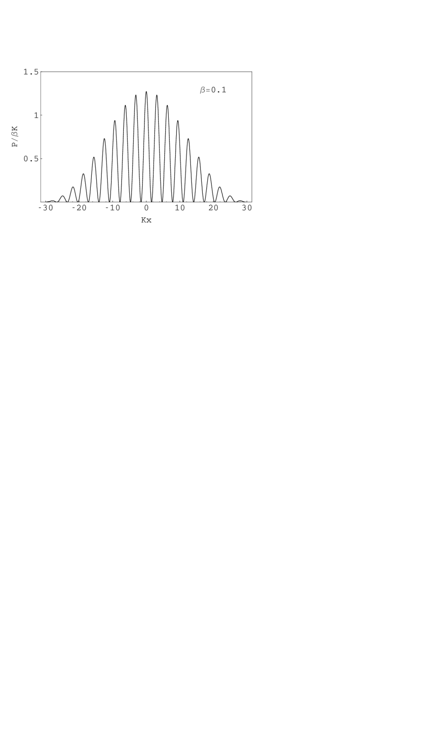
Figure 2: Two slit interference pattern.

3 Quantum Mechanics with Dissipation

The need to double the degrees of freedom of a Brownian motion particle is implicit even in the classical theory. Recall that in the classical Brownian theory one employs the equation of motion

$$M\ddot{x}(t)+R\dot{x}(t)=f(t),$$ (28)

where $f(t)$ is a random (Gaussian distributed) force obeying

$$<f(t)f(t^{\prime})>_{noise}=2\,R\,k_{B}T\;\delta(t-t^{\prime}).$$ (29)

To enforce Eq.(28) one can employ a delta functional classical constraint representation as a functional integral

$$\delta[M\ddot{x}+R\dot{x}-f]=\int{\cal D}y\;\exp\left[{i\over\hbar}\,\int dt\;y\{f-M\ddot{x}-R\dot{x}\}\right].$$ (30)

Note in Eq.(30) that one needs a constant $\hbar$ with dimensions of action which from purely classical considerations cannot be fixed in magnitude. From the viewpoint of quantum mechanics, we know how to fix the magnitude. (Exactly the same situation prevails in the purely classical statistical mechanics of Gibbs. The dimensionless phase space volume is $\Pi_{k}(dp_{k}dq_{k}/2\pi\hbar)$ and the precise value to be chosen for the action quantum $2\pi\hbar$ was evident only after quantum theory.)

Integration by parts in the time integral of Eq.(30), and averaging over the fluctuating force $f$ yields

$$<\delta[M\ddot{x}+R\dot{x}-f]>_{noise}=\int{\cal D}y<\exp\left[{i\over\hbar}\int dt\;{\cal L}_{f}(\dot{x},\dot{y},x,y)\right]>_{noise},$$ (31)

where

$${\cal L}_{f}(\dot{x},\dot{y},x,y)=M\dot{x}\dot{y}+{R\over 2}(x\dot{y}-y\dot{x})+fy.$$ (32)

At the classical level, the constraint condition introduced a new coordinate $y$, and from a Lagrangian viewpoint

$${d\over dt}{\partial{\cal L}_{f}\over\partial\dot{y}}={\partial{\cal L}_{f}\over\partial y}\quad;\ \ \ {d\over dt}{\partial{\cal L}_{f}\over\partial\dot{x}}={\partial{\cal L}_{f}\over\partial x},$$ (33)

i.e.

$$M\ddot{x}+R\dot{x}=f\quad;\ \ \ M\ddot{y}-R\dot{y}=0.$$ (34)

It is in fact true that the Lagrangian system Eqs.(32)-(34) were discovered from a completely classical viewpoint [7]. In the $x$ coordinate there is damping, but in the $y$ coordinate there is amplification.

Although the Lagrangian Eq.(32) was not here motivated by quantum mechanics, it is a simple matter to make contact with the theory of a quantum Brownian particle moving in a classical fluid using the transformation [4]

$$x_{\pm}=x\pm{y\over 2}.$$ (35)

In this case, after averaging over the random force using

$$<\exp\left[{i\over\hbar}\int dt\;y(t)f(t)\right]>_{noise}=\exp\left[-{k_{B}TR\over\hbar^{2}}\int dt\;y(t)^{2}\right],$$ (36)

one finds

$$<\exp\left[{i\over\hbar}\int dt\;{\cal L}_{f}(\dot{x},\dot{y},x,y)\right]>_{noise}=\exp\left[{i\over\hbar}\int dt\;{\cal L}(\dot{x}_{+},\dot{x}_{-},x_{+},x_{-})\right],$$ (37)

with a complex Lagrangian

$${\cal L}(\dot{x}_{+},\dot{x}_{-},x_{+},x_{-})={M\over 2}(\dot{x}_{+}^{2}-\dot{x}_{-}^{2})+{R\over 2}(\dot{x}_{+}x_{-}-\dot{x}_{-}x_{+})\,+\,i{k_{B}TR\over\hbar}(x_{+}-x_{-})^{2},$$ (38)

In evaluating Eq.(36) we employed Eq.(29) and the Gaussian nature of the random force. Considered as a statistical probability in the coordinate $y$, Eq.(29) represents a Gaussian process with a correlation function given in Eq.(12). Employing the Lagrangian in Eq.(38) in a path integral formulation for the density matrix [2, 8],

$$(x_{+}|\rho(t)|x_{-})=\int_{-\infty}^{\infty}\int_{-\infty}^{\infty}K(x_{+},x_{+}^{\prime},x_{-},x_{-}^{\prime},t)\,(x_{+}^{\prime}|\rho_{0}|x_{-}^{\prime})\;dx_{+}^{\prime}dx_{-}^{\prime},$$ (39)

and

$$K(x_{+},x_{+}^{\prime},x_{-},x_{-}^{\prime},t)=\int_{x_{+}^{\prime}}^{x_{+}}{\cal D}x_{+}(t^{\prime})\int_{x_{-}^{\prime}}^{x_{-}}{\cal D}x_{-}(t^{\prime})\ \exp\left[{i\over\hbar}\int_{0}^{t}{\cal L}^{\prime}dt^{\prime}\right],$$ (40)

yields the equation of motion (11).

Note, from Eqs.(9)-(11) the normalization integral

$$N(t)=Tr\rho(t)=\int_{-\infty}^{\infty}\int_{-\infty}^{\infty}\delta(x_{+}-x_{-})\;(x_{+}|\rho(t)|x_{-})\;dx_{+}dx_{-}$$ (41)

obeys

$$\dot{N}(t)=-{R\over 2M}N(t)\ ,\ \ \ \ N(t)=N(0)e^{-\frac{R}{2M}t}.$$ (42)

The decay of the normalization is a consequence of the customary procedure of integrating out an infinite number of thermal Brownian motion bath coordinates in statistical mechanics. This process gives rise to an effective Hamiltonian ${\cal H}_{Brownian}$ which even in the limit $T\to 0$ is not self adjoint; i.e. with

$${\cal H}_{0}=\lim_{T\to 0}\ {\cal H}_{Brownian},$$ (43)

the eigenvalues of ${\cal H}_{0}$ are complex [9, 10]. These complex eigenvalues lead to the (temperature independent) decay of $N(t)$. To keep the probability “normalized” one merely uses the average $<A>=(tr(\rho A)/tr\rho)$.

At zero temperature, the equation of motion for the density matrix is given by

$$i\hbar{\partial(x_{+}|\rho(t)|x_{-})\over\partial t}={\cal H}_{0}\ (x_{+}|\rho(t)|x_{-}),$$ (44)

$${\cal H}_{0}\ =\frac{1}{2M}\left(p_{+}-\frac{R}{2}\,x_{-}\right)^{2}-\frac{1}{2M}\left(p_{-}+\frac{R}{2}\,x_{+}\right)^{2}.$$ (45)

The solution to Eq.(44) has the form

$$(x_{+}|\rho(t)|x_{-})=\int_{-\infty}^{\infty}\int_{-\infty}^{\infty}K_{0}(x_{+},x_{+}^{\prime},x_{-},x_{-}^{\prime},t)\,(x_{+}^{\prime}|\rho_{0}|x_{-}^{\prime})\;dx_{+}^{\prime}dx_{-}^{\prime},$$ (46)

where

$$K_{0}(x_{+},x_{+}^{\prime},x_{-},x_{-}^{\prime},t)=e^{-i{\cal H}_{0}t/\hbar}\delta(x_{+}-x_{+}^{\prime})\delta(x_{-}-x_{-}^{\prime}),$$ (47)

or, in path integral form

$$K_{0}(x_{+},x_{+}^{\prime},x_{-},x_{-}^{\prime},t)=\int_{x_{+}^{\prime}}^{x_{+}}{\cal D}x_{+}(s)\int_{x_{-}^{\prime}}^{x_{-}}{\cal D}x_{-}(s)\ \exp\left[{i\over\hbar}\int_{0}^{t}{\cal L}_{0}(s)ds\right],$$ (48)

where

$${\cal L}_{0}(s)={M\over 2}\Big{[}\dot{x}_{+}^{2}(s)-\dot{x}_{-}^{2}(s)\Big{]}+{R\over 2}\Big{[}\dot{x}_{+}(s)x_{-}(s)-\dot{x}_{-}(s)x_{+}(s)\Big{]}.$$ (49)

From Eqs.(48), (49), a translation of the coordinates by a constant $(x_{+},x_{-})\to(x_{+}+a_{+},x_{-}+a_{-})$ yields

$$K_{0}(x_{+}+a_{+},x_{+}^{\prime}+a_{+},x_{-}+a_{-},x_{-}^{\prime}+a_{-},t)=\hskip 227.62204pt$$

$$\hskip 113.81102pt\exp\left[{iR\over 2\hbar}\Big{(}a_{-}(x_{+}-x_{+}^{\prime})-a_{+}(x_{-}-x_{-}^{\prime})\Big{)}\right]K_{0}(x_{+},x_{+}^{\prime},x_{-},x_{-}^{\prime},t).$$ (50)

From Eq.(50),

$$K_{0}(x_{+},x_{+}^{\prime},x_{-},x_{-}^{\prime},t)=e^{i\Phi(x_{+},x_{-},x_{+}^{\prime},x_{-}^{\prime})}{\cal F}_{0}(x_{+}-x_{+}^{\prime},x_{-}-x_{-}^{\prime},t),$$ (51)

where

$$\Phi(x_{+},x_{-},x_{+}^{\prime},x_{-}^{\prime})={R\over 2\hbar}(x_{+}x_{-}^{\prime}-x_{-}x_{+}^{\prime}).$$ (52)

From

$$i\hbar{\partial K_{0}(x_{+},x_{+}^{\prime},x_{-},x_{-}^{\prime},t)\over\partial t}={\cal H}_{0}\ K_{0}(x_{+},x_{+}^{\prime},x_{-},x_{-}^{\prime},t),$$ (53)

and Eq.(51) one finds

$$i\hbar{\partial{\cal F}_{0}(x_{+},x_{-},t)\over\partial t}=\left[\frac{1}{2M}\left(p_{+}-\frac{R}{2}\,x_{-}\right)^{2}\,-\,\frac{1}{2M}\left(p_{-}+\frac{R}{2}\,x_{+}\right)^{2}\right]{\cal F}_{0}(x_{+},x_{-},t).$$ (54)

With

$$\gamma=\frac{R}{2M},$$ (55)

the solution of Eq.(54) is given by

$${\cal F}_{0}(x_{+},x_{-},t)={M\gamma\over 2\pi\hbar\ \sinh(\gamma t)}\exp\left[\frac{i}{2\hbar}M\,\gamma\ \coth(\gamma t)(x_{+}^{2}-x_{-}^{2})\right].$$ (56)

4 Phase Coherence and Dissipative Flux

The above results may be applied to the two slit diffraction problem as in Eq.(19). The general result is that the probability density in $x$ is given by

$$P(x,t)=\int_{-\infty}^{\infty}\int_{-\infty}^{\infty}K(x,x_{+},x,x_{-},t)\,(x_{+}|\rho_{0}|x_{-})\;dx_{+}dx_{-}.$$ (57)

In the regime of Eq.(21) we then obtain from Eqs.(51),(52) and (55)-(57) and the renormalized time $\tau$

$$\gamma\tau=e^{-\gamma t}\sinh(\gamma t),$$ (58)

$$e^{\gamma t}P_{0}(x,t)\approx{M\over 2\pi\hbar\tau}\int_{-\infty}^{\infty}\int_{-\infty}^{\infty}\exp\left[-\frac{iM}{\hbar\tau}\,x\,(x_{+}-x_{-})\right](x_{+}|\rho_{0}|x_{-})\;dx_{+}dx_{-}.$$ (59)

Comparing Eq.(21) to Eq.(59) one finds the following remarkable result: For a particle in a bath which induces a damping $\gamma=(R/2M)$ at zero temperature, the slit diffraction patterns for the frictional case can be obtained from those of the zero friction case. All that is required is to rescale the effective time according to Eq.(58).

The probability density (at zero temperature) to find a particle in the interval $dx$ is proportional to

$$P(x,t)={M\gamma\over 2\pi\hbar\sinh(\gamma t)}\int_{-\infty}^{\infty}\int_{-\infty}^{\infty}\exp\left[i\,\phi(x,x_{+}-x_{-})+i\,{M\gamma(x_{+}^{2}-x_{-}^{2})\over 2\hbar\tanh(\gamma t)}\right](x_{+}|\rho_{0}|x_{-})\;dx_{+}dx_{-},$$ (60)

where

$$\phi(x,x_{+}-x_{-})=-{M\gamma\,x(x_{+}-x_{-})\over\hbar}=-{R\,x(x_{+}-x_{-})\over 2\hbar}.$$ (61)

Eqs.(60), (61) follow from Eqs.(51), (52) and (55)-(57).

The phase in Eq.(52), i.e. $\Phi(x_{+},x_{-},x_{+}^{\prime},x_{-}^{\prime})=(R/2\hbar)(x_{+}x_{-}^{\prime}-x_{-}x_{+}^{\prime})$ represents a “dissipative flux” $2\hbar\Phi=R\ Area$. With ${\bf X}=(x_{+},x_{-})$ and ${\bf X}^{\prime}=(x_{+}^{\prime},x_{-}^{\prime})$ as vectors in a plane, $Area={\bf N\cdot}({\bf X\times X}^{\prime})$, where ${\bf N}$ is the vector normal to the plane. The phase $\phi(x,x_{+}^{\prime}-x_{-}^{\prime})=\Phi(x_{+}=x,x_{-}=x,x_{+}^{\prime},x_{-}^{\prime})$ in Eqs. (60) and (61) is of the dissipative flux type.

Note the similarity between Eq.(45) and the Hamiltonian for a particle in the $x-y$ plane with a magnetic field in the z-direction; i.e. $H=({\bf p}-e\,{\bf B\times r}/2c)^{2}/2M$. For the magnetic field case, the flux is $B\times Area$ while for the closely analogous case of ${\cal H}_{0}$ the flux is $R\times Area$. Magnetic flux induces Aharonov-Bohm phase interference for the charged particle. Dissipative flux yields an analogous phase interference between forward and backward in time motion as expressed by mechanical damping. The similarity is most easily appreciated in the path integral formulation as in Eqs.(38) and (39), (40). The resistive part of the action is

$${\cal S}_{R}={R\over 2}\int(x_{-}\dot{x}_{+}-x_{+}\dot{x}_{-})dt={R\over 2}\int(x_{-}dx_{+}-x_{+}dx_{-}).$$ (62)

To see the phase interference for two different paths $P_{1}$ and $P_{2}$ in the $(x_{+},x_{-})$ plane with the same endpoints, one should compute (with $\int_{P_{1}}-\int_{P_{2}}=\oint$),

$${{\cal S}_{R}(\mbox{\footnotesize$interference$\normalsize})\over\hbar}={R\over 2\hbar}\oint(x_{-}dx_{+}-x_{+}dx_{-})={R\,\Sigma(P_{1},P_{2})\over\hbar},$$ (63)

where $\Sigma(P_{1},P_{2})$ is the oriented area between the two paths $P_{1}$ and $P_{2}$. Such phase interference $\exp\left[iR\,\Sigma/\hbar\right]$ enters into the path integral formulation of the problem in Eq.(48). The condition of constructive phase interference is thereby $R\,\Sigma=2\pi n\hbar$ where $n=0,\pm 1,\pm 2,...$ is a quantization integer.

5 Conclusions

In the conventional textbook description of quantum mechanics, one considers that there is but one coordinate $x$ (or more generally one set of coordinates) which describes a physical system. As shown by Schwinger (in his seminal work on Brownian motion [2]), in quantum mechanical theory it is often more natural to consider doubling the system coordinates, in our case from one coordinate $x(t)$ describing motion in time to two coordinates, say $x_{+}(t)$ going forward in time and $x_{-}(t)$ going backward in time.

In this picture, a system acts in a classical fashion if the two paths can be identified, i.e. $x_{classical}(t)\equiv x_{+\ classical}(t)\equiv x_{-\ classical}(t)$. When the system moves so that the forward in time and backward in time motions are (at the same time) unequal $x_{+}(t)\neq x_{-}(t)$, then the system is behaving in a quantum mechanical fashion and exhibits interference patterns in measured position probability densities. Of course when $x$ is actually measured there is only one classical $x=x_{+}=x_{-}$.

It is only when you do not look at a coordinate, e.g. do not look at which slit the electron may have passed, that the quantum picture is valid $x_{+}\neq x_{-}$. In this fascinating regime in which coordinate doubling and path splitting takes place, we are all under the dictates of Bohr who finally warns us not to ask what the quantum system is really doing. When the system is quantum mechanical just add up the amplitudes and absolute square them. Ask nothing more.

In this work we have concentrated on the low temperature limit, which means $T\ll T_{\gamma}$ where

$$k_{B}T_{\gamma}=\hbar\gamma={\hbar R\over 2M}.$$ (64)

In the high temperature regime $T\gg T_{\gamma}$, the thermal bath motion suppresses the probability for $x_{+}\neq x_{-}$ via the thermal term $(k_{B}TR/\hbar)(x_{+}-x_{-})^{2}$ in Eq.(9). In terms of the diffusion coefficient in Eqs.(1) and (64), i.e.

$$D={T\over T_{\gamma}}\Big{(}{\hbar\over 2M}\Big{)},$$ (65)

the condition for classical Brownian motion for high mass particles is that $D\gg(\hbar/2M)$, and the condition for quantum interference with low mass particles is that $D\ll(\hbar/2M)$. For a single atom in a fluid at room temperature it is typically true that $D\sim(\hbar/2M)$, equivalently $T\sim T_{\gamma}$ so that quantum mechanics plays an important but perhaps not dominant role in the Brownian motion. For large particles (in, say, colloidal systems) classical Brownian motion would appear to dominate the motion. It is interesting to note that in the formulation of quantum mechanics known as stochastic quantization, $(\hbar/2M)$ plays the role of a diffusion coefficient of a sort defined by Nelson [11] which also distinguishes forward and backwards in time splitting. In such a formulation the distinction between low temperature quantum motions and high temperature classical motions would become the distinction between Nelson diffusion and Einstein diffusion.

It is remarkable that, although in different contexts and in different view point frameworks, coordinate doubling has also entered into the canonical quantization of finite temperature field theoretical systems [12] as well as other dissipative systems [9, 10] and it appears to be intimately related to the algebraic properties of the theory [13, 14].

Finally, we note that the ”negative” kinematic term in the Lagrangian (38) also appears in two-dimensional gravity models leading to (at least) two different strategies in the quantization method [15]: the Schrödinger representation approach, where no negative norm appears, and the string/conformal field theory approach where negative norm states arise as in Gupta-Bleurer electrodynamics. It appears to be an interesting question to ask about any deeper connection between the $(x_{+},x_{-})$ Schwinger formalism and the subtelties of low dimensional gravity theory.

We hope that the views discussed in this work have clarified the nature of coordinate doubling framework.

Acknowledgments

This work has been partially supported by DOE in USA, by INFN in Italy and by EU Contract ERB CHRX CT940423.

References

[1] A. Tonomura, J. Endo, T. Matsuda, T.Kawasaki and H. Exawa,
Amer. J. Phys.57 (1989), 117
[2] J. Schwinger, J. Math. Phys. 2 (1961), 407
[3] V.V. Dodonov, O.V. Man’ko and V.I. Man’ko, J. of
Russian Laser Research16 (1995), 1
[4] Y.N. Srivastava, G. Vitiello and A. Widom, Ann.
Phys. (N.Y.) 238 (1995), 200
[5] M. Blasone, E. Graziano, O.K. Pashaev and G. Vitiello,
Ann. Phys. (N.Y.)252 (1996), 115
[6] Y. Tsue, A. Kuriyama and M. Yamamura, Progr. Theor. Physics91 (1994), 469
[7] H. Bateman, Phys. Rev.38 (1931), 815
[8] R.P. Feynman and F.L. Vernon, Ann. Phys. (N.Y.)24 (1963), 118
[9] H. Feshbach and Y. Tikochinsky, Trans. New York Acad.
Sci. (Ser.II)38 (1977), 44
[10] E. Celeghini, M. Rasetti and G. Vitiello, Ann.
Phys. (N.Y.) 215 (1992), 156
[11] E. Nelson, Quantum Fluctuations (Princeton
University Press, Princeton, 1985)
[12] Y. Takahashi and H. Umezawa, Collective Phenomena 2 (1975), 55; U. Umezawa, M. Matsumoto and M. Tachiki,
Thermo Field Dynamics and Condensed States
(North-Holland, Amsterdam, 1982)
[13] S. De Martino, S. De Siena and G. Vitiello, Int. J. Mod.
Phys.B10 (1996), 1615
[14] A.E. Santana and F.C. Khanna, Phys. Lett.A203 (1995), 68
[15] R. Jackiw, Two lectures on two-dimensional gravity,
gr-qc/9511048; D. Cangemi, R. Jackiw and B. Zwiebach, Ann. Phys.
(N.Y.)245 (1996), 408