Fault-tolerant quantum computation by anyons

Abstract

A two-dimensional quantum system with anyonic excitations can be considered as a quantum computer. Unitary transformations can be performed by moving the excitations around each other. Measurements can be performed by joining excitations in pairs and observing the result of fusion. Such computation is fault-tolerant by its physical nature.

A quantum computer can provide fast solution for certain computational problems (e.g. factoring and discrete logarithm [1]) which require exponential time on an ordinary computer. Physical realization of a quantum computer is a big challenge for scientists. One important problem is decoherence and systematic errors in unitary transformations which occur in real quantum systems. From the purely theoretical point of view, this problem has been solved due to Shor’s discovery of fault-tolerant quantum computation [2], with subsequent improvements [3, 4, 5, 6]. An arbitrary quantum circuit can be simulated using imperfect gates, provided these gates are close to the ideal ones up to a constant precision $\delta$. Unfortunately, the threshold value of $\delta$ is rather small; it is very difficult to achieve this precision.

Needless to say, classical computation can be also performed fault-tolerantly. However, it is rarely done in practice because classical gates are reliable enough. Why is it possible? Let us try to understand the easiest thing — why classical information can be stored reliably on a magnetic media. Magnetism arise from spins of individual atoms. Each spin is quite sensitive to thermal fluctuations. But the spins interact with each other and tend to be oriented in the same direction. If some spin flips to the opposite direction, the interaction forces it to flip back to the direction of other spins. This process is quite similar to the standard error correction procedure for the repetition code. We may say that errors are being corrected at the physical level. Can we propose something similar in the quantum case? Yes, but it is not so simple. First of all, we need a quantum code with local stabilizer operators.

I start with a class of stabilizer quantum codes associated with lattices on the torus and other 2-D surfaces [6, 8]. Qubits live on the edges of the lattice whereas the stabilizer operators correspond to the vertices and the faces. These operators can be put together to make up a Hamiltonian with local interaction. (This is a kind of penalty function; violating each stabilizer condition costs energy). The ground state of this Hamiltonian coincides with the protected space of the code. It is $4^{g}$-fold degenerate, where $g$ is the genus of the surface. The degeneracy is persistent to local perturbation. Under small enough perturbation, the splitting of the ground state is estimated as $\exp(-aL)$, where $L$ is the smallest dimension of the lattice. This model may be considered as a quantum memory, where stability is attained at the physical level rather than by an explicit error correction procedure.

Excitations in this model are anyons, meaning that the global wavefunction acquires some phase factor when one excitation moves around the other. One can operate on the ground state space by creating an excitation pair, moving one of the excitations around the torus, and annihilating it with the other one. Unfortunately, such operations do not form a complete basis. It seems this problem can be removed in a more general model (or models) where the Hilbert space of a qubit have dimensionality $>2$. This model is related to Hopf algebras.

In the new model, we don’t need torus to have degeneracy. An $n$-particle excited state on the plane is already degenerate, unless the particles (excitations) come close to each other. These particles are nonabelian anyons, i.e. the degenerate state undergoes a nontrivial unitary transformation when one particle moves around the other. Such motion (“braiding”) can be considered as fault-tolerant quantum computation. A measurement of the final state can be performed by joining the particles in pairs and observing the result of fusion.

Anyons have been studied extensively in the field-theoretic context [9, 10, 11, 12, 13]. So, I hardly discover any new about their algebraic properties. However, my approach differs in several respects:

• The model Hamiltonians are different.

• We allow a generic (but weak enough) perturbation which removes any symmetry of the Hamiltonian.

• The language of ribbon and local operators (see Sec. 5.2) provides unified description of anyonic excitations and long range entanglement in the ground state.

An attempt to use one-dimensional anyons for quantum computation was made by G. Castagnoli and M. Rasetti [14], but the question of fault-tolerance was not considered.

1 Toric codes and the corresponding Hamiltonians

Consider a $k\times k$ square lattice on the torus (see fig. 1). Let us attach a spin, or qubit, to each edge of the lattice. (Thus, there are $n=2k^{2}$ qubits). For each vertex $s$ and each face $p$, consider operators of the following form

$$A_{s}\ =\ \prod_{j\in\mbox{\scriptsize star}(s)}\sigma^{x}_{j}\qquad\qquad B_{p}\ =\ \prod_{j\in\mbox{\scriptsize boundary}(p)}\sigma^{z}_{j}$$ (1)

These operators commute with each other because $\mbox{star}(s)$ and $\mbox{boundary}(p)$ have either 0 or 2 common edges. The operators $A_{s}$ and $B_{p}$ are Hermitian and have eigenvalues $1$ and $-1$.

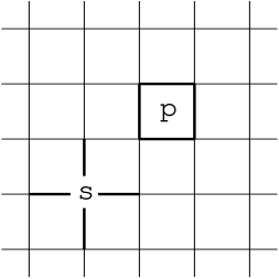
Figure 1: Square lattice on the torus

Let $\mathcal{N}$ be the Hilbert space of all $n=2k^{2}$ qubits. Define a protected subspace $\mathcal{L}\subseteq\mathcal{N}$ as follows

$$\mathcal{L}\ =\ \Bigl{\{}\,|\xi\rangle\in\mathcal{N}\,:\,\ A_{s}|\xi\rangle=|\xi\rangle,\ B_{p}|\xi\rangle=|\xi\rangle\ \mbox{for all}\ s,p\,\Bigr{\}}$$ (2)

This construction gives us a definition of a quantum code $\mathop{\mathrm{missing}}{TOR}\nolimits(k)$, called a toric code [6, 8]. The operators $A_{s}$, $B_{p}$ are the stabilizer operators of this code.

To find the dimensionality of the subspace $\mathcal{L}$, we can observe that there are two relations between the stabilizer operators,  $\prod_{s}A_{s}=1$  and $\prod_{p}B_{p}=1$. So, there are $m=2k^{2}-2$ independent stabilizer operators. It follows from the general theory of additive quantum codes [15, 16] that  $\dim\mathcal{L}=2^{n-m}=4$.

However, there is a more instructive way of computing $\dim\mathcal{L}$. Let us find the algebra $\mathbf{L}(\mathcal{L})$ of all linear operators on the space $\mathcal{L}$ — this will give us full information about this space. Let $\mathcal{F}\subseteq\mathbf{L}(\mathcal{N})$ be the algebra of operators generated by $A_{s}$, $B_{p}$. Clearly, $\mathbf{L}(\mathcal{L})\cong\mathcal{G}/\mathcal{I}$,  where $\mathcal{G}\supseteq\mathcal{F}$ is the algebra of all operators which commute with $A_{s}$, $B_{p}$,  and $\mathcal{I}\subset\mathcal{G}$ is the ideal generated by $A_{s}\!-\!1$,  $B_{p}\!-\!1$. The algebra $\mathcal{G}$ is generated by operators of the form

$$Z\ =\ \prod_{j\in c}\sigma^{z}_{j}\qquad\qquad X\ =\ \prod_{j\in c^{\prime}}\sigma^{x}_{j}$$

where $c$ is a loop (closed path) on the lattice, whereas $c^{\prime}$ is a cut, i.e. a loop on the dual lattice (see fig. 2). If a loop (or a cut) is contractible then the operator $Z$ is a product of $B_{p}$, hence $Z\equiv 1\pmod{\mathcal{I}}$. Thus, only non-contractible loops or cuts are interesting. It follows that the algebra $\mathbf{L}(\mathcal{L})$ is generated by 4 operators $Z_{1}$, $Z_{2}$, $X_{1}$, $X_{2}$ corresponding to the loops $c_{z1}$, $c_{z2}$ and the cuts $c_{x1}$, $c_{x2}$ (see fig. 2). The operators $Z_{1}$, $Z_{2}$, $X_{1}$, $X_{2}$ have the same commutation relations as $\sigma^{z}_{1}$, $\sigma^{z}_{2}$, $\sigma^{x}_{1}$, $\sigma^{x}_{2}$. We see that each quantum state $|\xi\rangle\in\mathcal{L}$ corresponds to a state of 2 qubits. Hence, the protected subspace $\mathcal{L}$ is 4-dimensional.

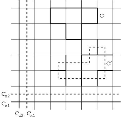
Figure 2: Loops on the lattice and the dual lattice

In a more abstract language, the algebra $\mathcal{F}$ corresponds to $2$-boundaries and $0$-coboundaries (with coefficients from $\mathbb{Z}_{2}$), $\mathcal{G}$ corresponds to $1$-cycles and $1$-cocycles, and $\mathbf{L}(\mathcal{L})$ corresponds to $1$-homologies and $1$-cohomologies.

There is also an explicit description of the protected subspace which may be not so useful but is easier to grasp. Let us choose basis vectors in the Hilbert space $\mathcal{N}$ by assigning a label $z_{j}=0,1$ to each edge $j$.  The constraints $B_{p}|\xi\rangle=|\xi\rangle$ say that the sum of the labels at the boundary of a face should be zero $(\bmod\ 2)$. More exactly, only such basis vectors contribute to a vector from the protected subspace. Such a basis vector is characterized by two topological numbers: the sums of $z_{j}$ along the loops $c_{z1}$ and $c_{z2}$. The constraints $A_{p}|\xi\rangle=|\xi\rangle$ say that all basis vectors with the same topological numbers enter $|\xi\rangle$ with equal coefficients. Thus, for each of the $4$ possible combinations of the topological numbers $v_{1},v_{2}$, there is one vector from the protected subspace,

$$|\xi_{v_{1},v_{2}}\rangle\ =\ 2^{-(k^{2}-1)/2}\,\sum_{z_{1},\ldots,z_{n}}|z_{1},\ldots,z_{n}\rangle\quad:\qquad\sum_{j\in c_{z1}}z_{j}=v_{1},\quad\sum_{j\in c_{z2}}z_{j}=v_{2}$$ (3)

Of course, one can also create linear combinations of these vectors.

Now we are to show that the code $\mathop{\mathrm{missing}}{TOR}\nolimits(k)$ detects $k-1$ errors (hence, it corrects $\left\lfloor\frac{k-1}{2}\right\rfloor$ errors). Consider a multiple error

$$E\ =\ \sigma(\alpha_{1},\ldots,\alpha_{n};\,\beta_{1},\ldots,\beta_{n})\ =\,\ \prod_{j}(\sigma^{x}_{j})^{\alpha_{j}}\ \prod_{j}(\sigma^{z}_{j})^{\beta_{j}}\qquad(\alpha_{j},\beta_{j}=0,1)$$

This error can not be detected by syndrome measurement (i.e. by measuring the eigenvalues of all $A_{s}$, $B_{j}$) if and only if $E\in\mathcal{G}$. However, if $E\in\mathcal{F}$ then $E|\xi\rangle=|\xi\rangle$ for every $|\xi\rangle\in\mathcal{L}$. Such an error is not an error at all — it does not affect the protected subspace. The bad case is when $E\in\mathcal{G}$ but $E\not\in\mathcal{F}$. Hence, the support of $E$ should contain a non-contractible loop or cut. It is only possible if $|\mathop{\mathrm{missing}}{Supp}\nolimits(E)|\geq k$. (Here $\mathop{\mathrm{missing}}{Supp}\nolimits(E)$ is the set of $j$ for which $\alpha_{j}\not=0$ or $\beta_{j}\not=0$).

One may say that the toric codes have quite poor parameters. Well, they are not “good” codes in the sense of [17]. However, the code $\mathop{\mathrm{missing}}{TOR}\nolimits(k)$ corrects almost any multiple error of size $O(k^{2})$. (The constant factor in $O(\ldots)$ is related to the percolation problem). So, these codes work if the error rate is constant but smaller than some threshold value. The nicest property of the codes $\mathop{\mathrm{missing}}{TOR}\nolimits(k)$ is that they are local check codes. Namely,

1. Each stabilizer operators involves bounded number of qubits (at most $4$).

2. Each qubit is involved in a bounded number of stabilizer operators (at most $4$).

3. There is no limit for the number of errors that can be corrected.

Also, at a constant error rate, the unrecoverable error probability goes to zero as $\exp(-ak)$.

It has been already mentioned that error detection involves syndrome measurement. To correct the error, one needs to find its characteristic vector $(\alpha_{1},\ldots,\alpha_{n};\,\beta_{1},\ldots,\beta_{n})$ out of the syndrome. This is the usual error correction scheme. A new suggestion is to perform error correction at the physical level. Consider the Hamiltonian

$$H_{0}\ =\ -\sum_{s}A_{s}\,-\,\sum_{p}B_{p}$$ (4)

Diagonalizing this Hamiltonian is an easy job because the operators $A_{s}$, $B_{p}$ commute. In particular, the ground state coincides with the protected subspace of the code $\mathop{\mathrm{missing}}{TOR}\nolimits(k)$; it is 4-fold degenerate. All excited states are separated by an energy gap $\Delta E\geq 2$, because the difference between the eigenvalues of $A_{s}$ or $B_{p}$ equals $2$. This Hamiltonian is more or less realistic because in involves only local interactions. We can expect that “errors”, i.e. noise-induced excitations will be removed automatically by some relaxation processes. Of course, this requires cooling, i.e. some coupling to a thermal bath with low temperature (in addition to the Hamiltonian (4)).

Now let us see whether this model is stable to perturbation. (If not, there is no practical use of it). For example, consider a perturbation of the form

$$V\ =\ -\vec{h}\sum_{j}\vec{\sigma}_{j}\ -\ \sum_{j<p}J_{jp}(\vec{\sigma}_{j},\vec{\sigma}_{p})$$

It is important that the perturbation is local, i.e. each term of it contains a small number of $\sigma$ (at most 2). Let us estimate the energy splitting between two orthogonal ground states of the original Hamiltonian, $|\xi\rangle\in\mathcal{L}$ and $|\eta\rangle\in\mathcal{L}$. We can use the usual perturbation theory because the energy spectrum has a gap. In the $m$-th order of the perturbation theory, the splitting is proportional to  $\langle\xi|V^{m}|\eta\rangle$  or  $\langle\xi|V^{m}|\xi\rangle-\langle\eta|V^{m}|\eta\rangle$. However, both quantities are zero unless $V^{m}$ contains a product of $\sigma^{z}_{j}$ or $\sigma^{x}_{j}$ along a non-contractible loop or cut. Hence, the splitting appears only in the $\lceil k/2\rceil$-th or higher orders. As far as all things (like the number of the relevant terms in $V^{m}$) scale correctly to the thermodynamic limit, the splitting vanishes as $\exp(-ak)$. A simple physical interpretation of this result is given in the next section. (Of course, the perturbation should be small enough, or else a phase transition may occur).

Note that our construction is not restricted to square lattices. We can consider an arbitrary irregular lattice, like in fig. 6. Moreover, such a lattice can be drawn on an arbitrary 2-D surface. On a compact orientable surface of genus $g$, the ground state is $4^{g}$-fold degenerate. In this case, the splitting of the ground state is estimated as $\exp(-aL)$, where $L$ is the smallest dimension of the lattice. We see that the ground state degeneracy depends on the surface topology, so we deal with topological quantum order. On the other hand, there is a finite energy gap between the ground state and excited states, so all spatial correlation functions decay exponentially. This looks like a paradox — how do parts of a macroscopic system know about the topology if all correlations are already lost at small scales? The answer is that there is long-range entanglement  which can not be expressed by simple correlation functions like $\langle\sigma^{a}_{j}\sigma^{b}_{l}\rangle$. This entanglement reveals itself in the excitation properties we are going to discuss.

2 Abelian anyons

Let us classify low-energy excitations of the Hamiltonian (4). An eigenvector of this Hamiltonian is an eigenvector of all the operators $A_{s}$, $B_{p}$. An elementary excitation, or particle occurs if only one of the constraints  $A_{s}|\xi\rangle=|\xi\rangle$,   $B_{p}\xi\rangle=|\xi\rangle$  is violated. Because of the relations $\prod_{s}A_{s}=1$ and $\prod_{p}B_{p}=1$,  it is impossible to create a single particle. However, it is possible to create a two-particle state of the form $|\psi^{z}(t)\rangle=S^{z}(t)|\xi\rangle$ or $|\psi^{x}(t^{\prime})\rangle=S^{x}(t^{\prime})|\xi\rangle$, where $|\xi\rangle$ is an arbitrary ground state, and

$$S^{z}(t)\ =\ \prod_{j\in t}\sigma^{z}_{j}\qquad\qquad\quad S^{x}(t^{\prime})\ =\ \prod_{j\in t^{\prime}}\sigma^{x}_{j}$$ (5)

(see fig. 3). In the first case, two particles are created at the endpoints of the “string” (non-closed path) $t$. Such particles live on the vertices of the lattice. We will call them $z$-type particles, or “electric charges”. Correspondingly, $x$-type particles, or “magnetic vortices” live on the faces. The operators $S^{z}(t)$, $S^{x}(t^{\prime})$ are called string operators. Their characteristic property is as follows:  they commute with every $A_{s}$ and $B_{p}$, except for few ones (namely, 2) corresponding to the endpoints of the string. Note that the state $|\psi^{z}(t)\rangle=S^{z}(t)|\xi\rangle$ depends only on the homotopy class of the path $t$ while the operator $S^{z}(t)$ depends on $t$ itself.

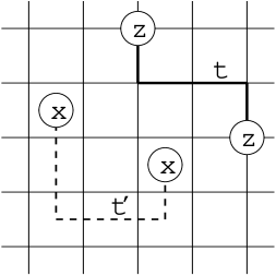
Figure 3: Strings and particles

Any configuration of an even number of $z$-type particles and an even number of $x$-type particles is allowed. We can connect them by strings in an arbitrary way. Each particle configuration defines a $4^{g}$-dimensional subspace in the global Hilbert space $\mathcal{N}$. This subspace is independent of the strings but a particular vector $S^{a_{1}}(t_{1})\cdots S^{a_{m}}(t_{m})|\xi\rangle$ depends on $t_{1},\ldots,t_{m}$. If we draw these strings in a topologically different way, we get another vector in the same $4^{g}$-dimensional subspace. Thus, the strings are unphysical but we can not get rid of them in our formalism.

Let us see what happens if these particles move around the torus (or other surface). Moving a $z$-type particle along the path $c_{z1}$ or $c_{z2}$ (see fig. 2) is equivalent to applying the operator $Z_{1}$ or $Z_{2}$. Thus, we can operate on the ground state space by creating a particle pair, moving one of the particles around the torus, and annihilating it with the other one. Thus we can realize some quantum gates. Unfortunately, too simple ones — we can only apply the operators $\sigma_{z}$ and $\sigma_{x}$ to each of the $2$ (or $2g$) qubits encoded in the ground state.

Now we can give the promised physical interpretation of the ground state splitting. In the presence of perturbation, the two-particle state $|\psi^{z}(t)\rangle$ is not an eigenstate any more. More exactly, both particles will propagate rather than stay at the same positions. The propagation process is described by the Schrödinger equation with some effective mass $m_{z}$. ($x$-type particles have another mass $m_{x}$). In the non-perturbed model, $m_{z}=m_{x}=\infty$. There are no real particles in the ground state, but they can be created and annihilate virtually. A virtual particle can tunnel around the torus before annihilating with the other one. Such processes contribute terms $b_{z1}Z_{1}$, $b_{z2}Z_{2}$, $b_{x1}X_{1}$, $b_{x2}X_{2}$ to the ground state effective Hamiltonian. Here $b_{\alpha i}\sim\exp(-a_{\alpha}L_{i})$ is the tunneling amplitude whereas $a_{\alpha}\sim\sqrt{2m\Delta\!E}$ is the imaginary wave vector of the tunneling particle.

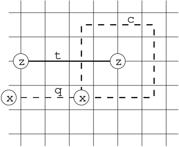
Figure 4: An $x$-type particle moving around a $z$-type particle

Next question: what happens if we move particles around each other? (For this, we don’t need a torus; we can work on the plane). For example, let us move an $x$-type particle around a $z$-type particle (see fig. 4). Then

$$|\Psi_{\mbox{\scriptsize initial}}\rangle\,=\,S^{z}(t)\,|\psi^{x}(q)\rangle\ ,\qquad\quad|\Psi_{\mbox{\scriptsize final}}\rangle\,=\,S^{x}(c)\,S^{z}(t)\,|\psi^{x}(q)\rangle\ =\ -|\Psi_{\mbox{\scriptsize initial}}\rangle$$

because $S^{x}(c)$ and $S^{z}(t)$ anti-commute, and $S^{x}(c)|\psi^{x}(q)\rangle=|\psi^{x}(q)\rangle$. We see that the global wave function ($=$ the state of the entire system) acquires the phase factor $-1$. It is quite unlike usual particles, bosons and fermions, which do not change their phase in such a process. Particles with this unusual property are called abelian anyons. More generally, abelian anyons are particles which realize nontrivial one-dimensional representations of (colored) braid groups. In our case, the phase change can be also interpreted as an Aharonov-Bohm effect. It does not occur if both particles are of the same type.

Note that abelian anyons exist in real solid state systems, namely, they are intrinsicly related to the fractional quantum Hall effect [18]. However, these anyons have different braiding properties. In the fractional quantum Hall system with filling factor $p/q$, there is only one basic type of anyonic particles with (real) electric charge $1/q$. (Other particles are thought to be composed from these ones). When one particle moves around the other, the wave function acquires a phase factor $\exp(2\pi i/q)$.

Clearly, the existence of anyons and the ground state degeneracy have the same nature. They both are manifestations of a topological quantum order, a hidden long-range order that can not be described by any local order parameter. (The existence of a local order parameter contradicts the nature of a quantum code — if the ground state is accessible to local measurements then it is not protected from local errors). It seems that the anyons are more fundamental and can be used as a universal probe for this hidden order. Indeed, the ground state degeneracy on the torus follows from the existence of anyons [19]. Here is the original Einarsson’s proof applied to our two types of particles.

We derived the ground state degeneracy from the commutation relations between the operators $Z_{1}$, $Z_{2}$, $X_{1}$, $X_{2}$. These operators can be realized by moving particles along the loops $c_{z1}$, $c_{z2}$, $c_{x1}$, $c_{x2}$. These loops only exist on the torus, not on the plane. Consider, however, the process in which an $x$-type particle and a $z$-type particle go around the torus and then trace their paths backward. This corresponds to the operator $W=X_{1}^{-1}Z_{1}^{-1}X_{1}Z_{1}$ which can be realized on the plane. Indeed, we can deform particles’ trajectories so that one particle stays at rest while the other going around it. Due to the anyonic nature of the particles, $W=-1$. We see that $X_{1}$ and $Z_{1}$ anti-commute.

The above argument is also applicable to the fractional quantum Hall anyons [19]. The ground state on the torus is $q$-fold degenerate, up to the precision $\sim\exp(-L/l_{0})$, where $l_{0}$ is the magnetic length. This result does not rely on the magnetic translational symmetry or any other symmetry. Rather, it relies on the existence of the energy gap in the spectrum (otherwise the degeneracy would be unstable to perturbation). Note that holes ($=$punctures) in the torus do not remove the degeneracy unless they break the nontrivial loops $c_{x1}$, $c_{x2}$, $c_{z1}$, $c_{z2}$. The fly-over crossing geometry (see fig. 5) is topologically equivalent to a torus with 2 holes, but it is almost flat. In principle, such structure can be manufactured , cooled down and placed into a perpendicular magnetic field. This will be a sort of quantum memory — it will store a quantum state forever, provided all anyonic excitation are frozen out or localized. Unfortunately, I do not know any way this quantum information can get in or out. Too few things can be done by moving abelian anyons. All other imaginable ways of accessing the ground state are uncontrollable.

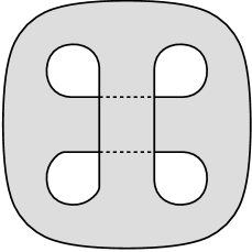
Figure 5: A fly-over crossing geometry for a 2-D electron layer

3 Materialized symmetry: is that a miracle?

Anyons have been studied extensively in the gauge field theory context [9, 10, 11, 13]. However, we start with quite different assumptions about the Hamiltonian. A gauge theory implies a gauge symmetry which can not be removed by external perturbation. To the contrary, our model is stable to arbitrary local perturbations. It is useful to give a field-theoretic interpretation of this model. The edge labels $z_{j}$ (measurable by $\sigma^{z}_{j}$) correspond to a $\mathbb{Z}_{2}$ vector potential, whereas $\sigma^{x}_{j}$ corresponds to the electric field. The operators $A_{s}$ are local gauge transformations whereas $B_{p}$ is the magnetic field on the face $p$. The constraints $A_{s}|\xi\rangle=|\xi\rangle$ mean that the state $|\xi\rangle$ is gauge-invariant. Violating the gauge invariance is energetically unfavorable but not forbidden. The Hamiltonian (which includes $H_{0}$ and some perturbation $V$) need not obey the gauge symmetry. The constraints $B_{p}|\xi\rangle=|\xi\rangle$ mean that the gauge field corresponds to a flat connection. These constraints are not strict either.

Despite the absence of symmetry in the Hamiltonian $H=H_{0}+V$, our system exhibits two conservation laws: electric charge and magnetic charge (i.e. the number of vortices) are both conserved modulo 2. In the usual electrodynamics, conservation of electric charge is related to the local ($=$gauge) $\mathbf{U}(1)$ symmetry. In our case, it should be a local $\mathbb{Z}_{2}$ symmetry for electric charges and another $\mathbb{Z}_{2}$ symmetry for magnetic vortices. So, our system exhibits a dynamically created $\mathbb{Z}_{2}\times\mathbb{Z}_{2}$ symmetry which appears only at large distances where individual excitations are well-defined.

Probably, the reader is not satisfied with this interpretation. Really, it creates a new puzzle rather than solve an old one. What is this mysterious symmetry? How do symmetry operators look like at the microscopic level? The answer sounds as nonsense but it is true. This symmetry (as well as any other local symmetry) can be found in any Hamiltonian if we introduce some unphysical degrees of freedom. So, the symmetry is not actually being created. Rather, an artificial symmetry becomes a real one.

The new degrees of freedom are spin variables $v_{s},w_{p}=0,1$ for each vertex $s$ and each face $p$. The vertex spins will stay in the state $2^{-1/2}\Bigl{(}|0\rangle+|1\rangle\Bigr{)}$ whereas the face spins will stay in the state $|0\rangle$. So, all the extra spins together stay in a unique quantum state $|\zeta\rangle$. Obviously, $\sigma^{x}_{s}|\zeta\rangle=|\zeta\rangle$ and $\sigma^{z}_{p}|\zeta\rangle=|\zeta\rangle$, for every vertex $s$ and every face $p$. From the mathematical point of view, we have simply defined an embedding of the space $\mathcal{N}$ into a larger Hilbert space $\mathcal{T}$ of all the spins,  $|\psi\rangle\mapsto|\psi\rangle\otimes|\zeta\rangle$. So we may write $\mathcal{N}\subseteq\mathcal{T}$. We will call $\mathcal{N}$ the physical space (or subspace), $\mathcal{T}$ the extended space. Physical states (i.e. vectors $|\psi\rangle\in\mathcal{N}$) are characterized by the equations

$$\sigma^{x}_{s}|\psi\rangle\,=\,|\psi\rangle\ ,\quad\ \sigma^{z}_{p}|\psi\rangle\,=\,|\psi\rangle\ \qquad\quad$$

for every vertex $s$ and face $p$.

Now let us apply a certain unitary transformation $U$ on the extended space $\mathcal{T}$. This transformation is just a change of the spin variables, namely

$$v_{s}\ \mapsto\ v_{s}\ ,\qquad\ z_{j}\ \mapsto\ z_{j}\,+\sum_{s=\mbox{\scriptsize endpoint}(j)}v_{s}\ ,\qquad\ w_{p}\ \mapsto\ w_{p}\,+\sum_{j\in\mbox{\scriptsize boundary}(p)}z_{j}$$ (6)

(all sums are taken modulo 2). The physical subspace becomes $\mathcal{N}^{\prime}=U\mathcal{N}$. Vectors $|\psi\rangle\in\mathcal{N}^{\prime}$ are invariant under the following symmetry operators

$$P_{s}\,=\,U\sigma^{x}_{s}U^{\dagger}\,=\ \sigma^{x}_{s}\,A_{s}\qquad\qquad Q_{p}\,=\,U\sigma^{z}_{p}U^{\dagger}\,=\ \sigma^{z}_{p}\,B_{p}$$ (7)

The transformed Hamiltonian $H^{\prime}=UHU^{\dagger}$ commutes with these operators. It is defined up to the equivalence  $P_{s}\equiv 1$,   $Q_{p}\equiv 1$. In particular,

$$H_{0}^{\prime}\ =\ U\,H_{0}\,U^{\dagger}\ =\ H_{0}^{\prime}\ \equiv\ -\sum_{s}\sigma^{x}_{s}\,-\sum_{p}\sigma^{z}_{p}$$ (8)

In the field theory language, the vertex variables $v_{s}$ (or the operators $\sigma^{z}_{s}$) are a Higgs field. The operators $P_{s}$ are local gauge transformations. Thus, an arbitrary Hamiltonian can be written in a gauge-invariant form if we introduce additional Higgs fields. Of course, it is a very simple observation. The real problem is to understand how the artificial gauge symmetry “materialize”, i.e. give rise to a physical conservation law.

Electric charge at a vertex $s$ is given by the operator $\sigma^{x}_{s}$. The total electric charge on a compact surface is zero because $\prod_{s}\sigma^{x}_{s}\equiv 1$. This is not a physically meaningful statement as it is. It is only meaningful if there are discrete charged particles. Then the charge is also conserved locally, in every scattering or fusion process. It is difficult to formulate this property in a mathematical language, but, hopefully, it is possible. (The problem is that particles are generally smeared and can propagate. Physically, particles are well-defined if they are stable and have finite energy gap). Alternatively, one can use various local and nonlocal order parameters to distinguish between phases with an unbroken symmetry, broken symmetry or confinement.

The artificial gauge symmetry materialize for the Hamiltonian (8) but this is not the case for every Hamiltonian. Let us try to describe possible symmetry breaking mechanisms in terms of local order parameters. If the gauge symmetry is broken then there is a nonvanishing vacuum average of the Higgs field, $\phi(s)=\langle\sigma^{z}_{s}\rangle\not=0$. Electric charge is not conserved any more. In other words, there is a Bose condensate of charged particles. Although the second $\mathbb{Z}_{2}$ symmetry is formally unbroken, free magnetic vortices do not exist. More exactly, magnetic vortices are confined. (The duality between symmetry breaking and confinement is well known [25]). It is also possible that the second symmetry is broken, then electric charges are confined. From the physical point of view, these two possibilities are equivalent: there is no conservation law in the system.

An interesting question is whether magnetic vortices can be confined without the gauge symmetry being broken. Apparently, the answer is “no”. The consequence is significant: electric charges and magnetic vortices can not exist without each other. It seems that materialized symmetry needs better understanding; as presented here, it looks more like a miracle.

4 The model based on a group algebra

From now on, we are constructing and studying nonabelian anyons which will allow universal quantum computation.

Let $G$ be a finite (generally, nonabelian) group. Denote by $\mathcal{H}=\mathbb{C}[G]$ the corresponding group algebra, i.e. the space of formal linear combinations of group elements with complex coefficients. We can consider $\mathcal{H}$ as a Hilbert space with a standard orthonormal basis $\Bigl{\{}|g\rangle:\,g\in G\Bigr{\}}$. The dimensionality of this space is $N=|G|$. We will work with “spins” (or “qubits”) taking values in this space. Remark: This model can be generalized. One can take for $\mathcal{H}$ any finite-dimensional Hopf algebra equipped with a Hermitian scalar product with certain properties. However, I do not want to make things too complicated.

To describe the model, we need to define 4 types of linear operators, $L_{+}^{g}$, $L_{-}^{g}$, $T_{+}^{h}$, $T_{-}^{h}$ acting on the space $\mathcal{H}$. Within each type, they are indexed by group elements, $g\in G$ or $h\in G$. They act as follows

$$\begin{array}[]{rclcrcl}L_{+}^{g}|z\rangle&=&|gz\rangle&&T_{+}^{h}|z\rangle&=&\delta_{h,z}\,|z\rangle\vskip 6.0pt plus 2.0pt minus 2.0pt\\ L_{-}^{g}|z\rangle&=&|zg^{-1}\rangle&&T_{-}^{h}|z\rangle&=&\delta_{h^{-1}\!,\,z}\,|z\rangle\end{array}$$ (9)

(In the Hopf algebra context, the operators $L_{+}^{g}$, $L_{-}^{g}$, $T_{+}^{h}$, $T_{-}^{h}$ correspond to the left and right multiplications and left and right comultiplication, respectively). These operators satisfy the following commutation relations

$$\begin{array}[]{rclcrcl}L_{+}^{g}\,T_{+}^{h}&=&T_{+}^{gh}\,L_{+}^{g}&&L_{+}^{g}\,T_{-}^{h}&=&T_{-}^{hg^{-1}}L_{+}^{g}\vskip 6.0pt plus 2.0pt minus 2.0pt\\ L_{-}^{g}\,T_{+}^{h}&=&T_{+}^{hg^{-1}}L_{-}^{g}&&L_{-}^{g}\,T_{-}^{h}&=&T_{-}^{gh}\,L_{-}^{g}\end{array}$$ (10)

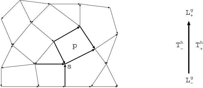
Figure 6: Generic lattice and the orientation rules for the operators $L^{g}_{\pm}$ and $T^{h}_{\pm}$

Now consider an arbitrary lattice on an arbitrary orientable 2-D surface, see fig. 6. (We will mostly work with a plane or a sphere, not higher genus surfaces). Corresponding to each edge is a spin which takes values in the space $\mathcal{H}$. Arrows in fig. 6 mean that we choose some orientation for each edge of the lattice. (Changing the direction of a particular arrow will be equivalent to the basis change $|z\rangle\mapsto|z^{-1}\rangle$ for the corresponding qubit). Let $j$ be an edge of the lattice, $s$ one of its endpoints. Define an operator $L^{g}(j,s)=L_{\pm}^{g}(j)$ as follows. If $s$ is the origin of the arrow $j$ then $L^{g}(j,s)$ is $L_{-}^{g}(j)$ (i.e. $L_{-}^{g}$ acting on the $j$-th spin), otherwise it is $L_{+}^{g}(j)$. This rule is represented by the diagram at the right side of fig. 6. Similarly, if $p$ is the left (the right) ajacent face of the edge $j$ then $T^{h}(j,p)$ is $T_{-}^{h}$ (resp. $T_{+}^{h}$) acting on the $j$-th spin.

Using these notations, we can define local gauge transformations and magnetic charge operators corresponding to a vertex $s$ and an adjacent face $p$ (see fig. 6). Put

$$\begin{array}[]{rcl}A_{g}(s,p)&=&A_{g}(s)\ =\ \prod\limits_{j\in\mbox{\scriptsize star}(s)}\,L^{g}(j,s)\vskip 6.0pt plus 2.0pt minus 2.0pt\\ B_{h}(s,p)&=&\sum\limits_{h_{1}\cdots h_{k}=h}\,\prod\limits_{m=1}^{k}\,T^{h_{m}}(j_{m},p)\end{array}$$ (11)

where $j_{1},\ldots,j_{k}$ are the boundary edges of $p$ listed in the counterclockwise order, starting from, and ending at, the vertex $s$. (The sum is taken over all combinations of $h_{1},\ldots,h_{k}\in G$, such that $h_{1}\cdots h_{k}=h$. Order is important here!). Although $A_{g}(s,p)$ does not depend on $p$, we retain this parameter to emphasize the duality between $A_{g}(s,p)$ and $B_{h}(s,p)$.  These operators generate an algebra $\mathcal{D}=\mathbf{D}(G)$, Drinfield’s quantum double [20] of the group algebra $\mathbb{C}[G]$. It will play a very important role below. Now we only need two symmetric combinations of $A_{g}(s,p)$ and $B_{h}(s,p)$, namely

$$A(s)\ =\ N^{-1}\sum_{g\in G}A_{g}(s,p)\qquad\qquad B(p)\ =\ B_{1}(s,p)$$ (12)

where $N=|G|$. Both $A(s)$ and $B(p)$ are projection operators. ($A(s)$ projects out the states which are gauge invariant at $s$, whereas $B(p)$ projects out the states with vanishing magnetic charge at $p$). The operators $A(s)$ and $B(p)$ commute with each other. Also $A(s)$ commutes with $A(s^{\prime})$, and $B(p)$ commutes with $B(p^{\prime})$ for different vertices and faces. In the case $G=\mathbb{Z}_{2}$, these operators are almost the same as the operators (1),  namely   $A(s)=\frac{1}{2}(A_{s}+1)$,    $B(p)=\frac{1}{2}(B_{p}+1)$. 

At this point, we have only defined the global Hilbert space $\mathcal{N}$ (the tensor product of many copies of $\mathcal{H}$) and some operators on it. Now let us define the Hamiltonian.

$$H_{0}\ =\ \sum_{s}(1-A(s))\,+\,\sum_{p}(1-B(p))$$ (13)

It is quite similar to the Hamiltonian (4). As in that case, the space of ground states is given by the formula

$$\mathcal{L}\ =\ \Bigl{\{}\,|\xi\rangle\in\mathcal{N}\,:\,\ A(s)|\xi\rangle=|\xi\rangle,\ B(p)|\xi\rangle=|\xi\rangle\ \mbox{for all}\ s,p\,\Bigr{\}}$$ (14)

The corresponding energy is $0$; all excited states have energies $\geq 1$.

It is easy to work out an explicit representation of ground states similar to eq. (3). The ground states correspond 1-to-1 to flat $G$-connections, defined up to conjugation, or superpositions of those. So, the ground state on a sphere is not degenerate. However, particles (excitations) have quite interesting properties even on the sphere or on the plane. (We treat the plane as an infinitely large sphere). The reader probably wants to know the answer first, and then follow formal calculations. So, I give a brief abstract description of these particles. It is a mixture of general arguments and details which require verification.

The particles live on vertices or faces, or both; in general, one particle occupies a vertex and an adjacent face same time. A combination of a vertex and an adjacent face will be called a site. Sites are represented by dotted lines in fig. 7. (The dashed lines are edges of the dual lattice).

Consider $n$ particles on the sphere pinned to particular sites $x_{1},\ldots,x_{n}$ at large distances from each other. The space $\mathcal{L}[n]=\mathcal{L}(x_{1},\ldots,x_{n})$ of $n$-particle states has dimensionality $N^{2(n-1)}$, including the ground state. Not all these states have the same energy. Even more splitting occurs under perturbation, but some degeneracy still survive. Of course, we assume that the perturbation is local, i.e. it can be represented by a sum of operators each of which acts only on few spins. To find the residual degeneracy, we will study the action of such local operators on the space $\mathcal{L}[n]$. Local operators generate a subalgebra $\mathcal{P}[n]\subseteq\mathbf{L}(\mathcal{L}[n])$. Elements of its center, $\mathcal{C}[n]$, are conserved classical quantities; they can be measured once and never change. (More exactly, they can not be changed by local operators). As these classical variables are locally measurable, we interpret them as particle’s types. It turns out that the types correspond 1-to-1 to irreducible representations of the algebra $\mathcal{D}$, the quantum double. Thus, each particle can belong to one of these types. The space $\mathcal{L}[n]$ and the algebra $\mathcal{P}[n]$ split accordingly:

$$\mathcal{L}[n]\ =\ \bigoplus_{d_{1},\ldots,d_{n}}\mathcal{L}_{d_{1},\ldots,d_{n}}\qquad\quad\mathcal{P}[n]\ =\ \bigoplus_{d_{1},\ldots,d_{n}}\mathcal{P}_{d_{1},\ldots,d_{n}}\qquad\quad\Bigl{(}\,\mathcal{P}_{d_{1},\ldots,d_{n}}\subseteq\mathbf{L}(\mathcal{L}_{d_{1},\ldots,d_{n}})\,\Bigr{)}$$ (15)

where $d_{m}$ is the type of the $m$-th particle. The “classical” subalgebra $\mathcal{C}[n]$ is generated by the projectors onto $\mathcal{L}_{d_{1},\ldots,d_{n}}$.

But this is not the whole story. The subspace $\mathcal{L}_{d_{1},\ldots,d_{n}}$ splits under local perturbations from $\mathcal{P}_{d_{1},\ldots,d_{n}}$. By a general mathematical argument, this algebra can be characterized as follows

$$\mathcal{L}_{d_{1},\ldots,d_{n}}\ =\ \mathcal{K}_{d_{1},\ldots,d_{n}}\otimes\mathcal{M}_{d_{1},\ldots,d_{n}}\qquad\qquad\mathcal{P}_{d_{1},\ldots,d_{n}}\ =\ \mathbf{L}(\mathcal{K}_{d_{1},\ldots,d_{n}})$$ (16)

The space $\mathcal{K}_{d_{1},\ldots,d_{n}}$ corresponds to local degrees of freedom. They can be defined independently for each particle. So,  $\mathcal{K}_{d_{1},\ldots,d_{n}}=\mathcal{K}_{d_{1}}\otimes\cdots\otimes\mathcal{K}_{d_{n}}$,  where $\mathcal{K}_{d_{m}}$ is the space of “subtypes” (internal states) of the $m$-th particle. Like the type, the subtype of a particle is accessible by local measurements. However, it can be changed, while the type can not.

The most interesting thing is the protected space $\mathcal{M}_{d_{1},\ldots,d_{n}}$. It is not accessible by local measurements and is not sensitive to local perturbations, unless the particles come close to each other. This is an ideal place to store quantum information and operate with it. Unfortunately, the protected space does not have tensor product structure. However, it can be described as follows. Associated with each particle type $a$ is an irreducible representation $\mathcal{U}_{d}$ of the quantum double $\mathcal{D}$. Consider the product representation $\mathcal{U}_{d_{1}}\otimes\cdots\otimes\mathcal{U}_{d_{n}}$ and split it into components corresponding to different irreducible representations. The protected space is the component corresponding to the identity representation.

If we swap two particles or move one around the other, the protected space undergoes some unitary transformation. Thus, the particles realize some multi-dimensional representation of the braid group. Such particles are called nonabelian anyons. Note that braiding does not affect the local degrees of freedom. If two particles fuse, they can annihilate or become another particle. The protected space becomes smaller but some classical information comes out, namely, the type of the new particle. So, the we can do measurements on the protected space. Finally, if we create a new pair of particles of definite types, it always comes in a particular quantum state. So, we have a standard toolkit for quantum computation (new states, unitary transformations and measurements), except that the Hilbert space does not have tensor product structure. Universality of this toolkit is a separate problem, see Sec. 7.

Our model gives rise to the same braiding and fusion rules as gauge field theory models [10, 11]. The existence of local degrees of freedom (subtypes) is a new feature. These degrees of freedom appear because there is no explicit gauge symmetry in our model.

5 Algebraic structure

5.1 Particles and local operators

This subsection is also rather abstract but the claims we do are concrete. They will be proven in Sec. 5.4.

As mentioned above, the ground state of the Hamiltonian (13) is not degenerate (on the sphere or on the plane regarded as an infinitely large sphere). Excited states are characterized by their energies. The energy of an eigenstate $|\psi\rangle$ is equal to the number of constraints $(A(s)-1)|\psi\rangle=0$ or $(B(p)-1)|\psi\rangle=0$ which are violated. Complete classification of excited states is a difficult problem. Instead of that, we will try to classify elementary excitations, or particles.

Let us formulate the problem more precisely. Consider a few excited “spots” separated by large distances. Each spot is a small region where some of the constrains are violated. The energy of a spot can be decreased by local operators but, generally, the spot can not disappear. Rather, it shrinks to some minimal excitation (which need not be unique). We will see (in Sec. 5.4) that any excited spot can be transformed into an excitation which violates at most 2 constraints,  $A(s)-1\equiv 0$ and $B(p)-1\equiv 0$,  where $s$ is an arbitrary vertex, and $p$ is an adjacent face. Such excitations are be called elementary excitations, or particles. Note that definition of elementary excitations is a matter of choice. We could decide that an elementary excitation violates 3 constraints. Even with our definition, the “space of elementary excitations” is redundant.

By the way, the space of elementary excitations is not well defined because such an excitation does not exist alone. More exactly, the only one-particle state on the sphere is the ground state. (This can be proven easily). The right thing is the space of two-particle excitations, $\mathcal{L}(a,b)$. Here $a=(s,p)$ and $b=(s^{\prime},p^{\prime})$ are the sites occupied by the particles. (Recall that a site is a combination of a vertex and an adjacent face). The projector onto $\mathcal{L}(a,b)$ can be written as $\prod_{r\not=s,s^{\prime}}A(r)\,\prod_{l\not=p,p^{\prime}}B(l)$. Note that introducing a third particle (say, $c$) will not give more freedom for any of the two. Indeed, $b$ and $c$ can fuse without any effect on $a$.

Let us see how local operators act on the space $\mathcal{L}(a,b)$. In this context, a local operator is an operator which acts only on spins near $a$ (or near $b$). Besides that, it should preserve the subspace $\mathcal{L}(a,b)\subseteq\mathcal{N}$ and its orthogonal complement. ($\mathcal{N}$ is the space of all quantum states). Example: the operators $A_{g}(a)$ and $B_{h}(a)$, where $a=(s,p)$, commute with $A(r)$, $B(l)$ for all $r\not=s$ and $l\not=p$. Hence, they commute with the projector onto the subspace $\mathcal{L}(a,b)$. These operators generate an algebra $\mathcal{D}(a)\subset\mathbf{L}(\mathcal{N})$. It will be shown in Sec. 5.4 that $\mathcal{D}(a)$ includes all local operators acting on the space $\mathcal{L}(a,b)$,  and the action of $\mathcal{D}(a)$ on $\mathcal{L}(a,b)$ is exact (i.e. different operators act differently).

Actually, the algebra $\mathcal{D}(a)=\mathcal{D}$ does not depend on $a$,  only the embedding $\mathcal{D}\to\mathbf{L}(\mathcal{N})$ does. This algebra is called the quantum double of the group $G$ and denoted by $\mathbf{D}(G)$. Its structure is determined by the following relations between the operators $A_{g}=A_{g}(a)$ and $B_{h}=B_{h}(a)$

$$A_{f}\,A_{g}\ =\ A_{fg}\qquad\qquad B_{h}\,B_{i}\ =\ \delta_{h,i}\,B_{h}\qquad\qquad A_{g}\,B_{h}\ =\ B_{ghg^{-1}}A_{g}$$ (17)

The operators $D_{(h,g)}=B_{h}A_{g}$ form a linear basis of $\mathcal{D}$. (In [10, 11] these operators were denoted by  $\raisebox{2.15277pt}{$\scriptstyle h$\,}{\mathop{\mbox{\rule{0.4pt}{7.74998pt}\rule{7.74998pt}{0.4pt}}}\limits_{g}}$ ). The following multiplication rules hold

$$D_{(h_{1},g_{1})}D_{(h_{2},g_{2})}\ =\ \delta_{h_{1},\,g_{1}h_{2}g_{1}^{-1}}\,D_{(h_{1},\,g_{1}g_{2})}$$

This identity can be also written in a symbolic tensor form, with $h$ and $g$ being combined into one index:

$$D_{\mbox{\scriptsize\boldmath$m$}}\,D_{\mbox{\scriptsize\boldmath$n$}}\ =\ {\Omega^{\mbox{\scriptsize\boldmath$k$}}_{\mbox{\scriptsize\boldmath$mn$}}}\,D_{\mbox{\scriptsize\boldmath$k$}}\qquad\qquad\quad\Omega^{(h,g)}_{(h_{1},g_{1})\,(h_{2},g_{2})}\ =\,\ \delta_{h_{1},\,g_{1}h_{2}g_{1}^{-1}}\ \delta_{h,h_{1}}\ \delta_{g,\,g_{1}g_{2}}$$ (18)

(summation over $k$ is implied). Actually, $\mathcal{D}$ is not only an algebra, it is a quasi-triangular Hopf algebra, see Secs. 5.2, 5.3.

Note that $\mathcal{D}=\mathcal{D}(a)$ is closed under Hermitian conjugation (in $\mathbf{L}(\mathcal{N})$) which acts as follows

$$A_{g}^{\dagger}\,=\,A_{g^{-1}}\qquad\qquad B_{h}^{\dagger}\,=\,B_{h}\qquad\qquad D_{(h,g)}^{\dagger}\,=\,D_{(g^{-1}hg,\,g^{-1})}$$ (19)

Thus, $\mathcal{D}=\mathcal{D}(a)$ is a finite-dimensional $C^{*}$-algebra. Hence it has the following structure

$$\mathcal{D}\ =\ \bigoplus_{d}\mathbf{L}(\mathcal{K}_{d})$$ (20)

where $d$ runs over all irreducible representations of $\mathcal{D}$. We can interpret $d$ as particle’s type. The absence of particle corresponds to a certain one-dimensional representation called the identity representation. More exactly, the operators $D_{(h,g)}$ act on the ground state $|\xi\rangle$ as follows

$$D_{\mbox{\scriptsize\boldmath$k$}}\,|\xi\rangle\ =\ \mbox{\large$\varepsilon$}_{\mbox{\scriptsize\boldmath$k$}}\,|\xi\rangle\qquad\qquad\mbox{where}\quad\mbox{\large$\varepsilon$}_{(h,g)}\ =\ \delta_{h,1}$$ (21)

The “space of subtypes”, $\mathcal{K}_{d}$ actually characterize the redundancy of our definition of elementary excitations. However, this redundancy is necessary to have a nice theory of ribbon operators (see Sec. 5.2).

Irreducible representations of $\mathcal{D}$ can be described as follows [10]. Let $u\in G$ be an arbitrary element, $C=\{gug^{-1}:\,g\in G\}$ its conjugacy class,  $E=\{g\in G:\,gu=ug\}$ its centralizer. There is one irreducible representation $d=(C,\chi)$ for each conjugacy class $C$ and each irreducible representation $\chi$ of the group $E$ (see below). It does not matter which element $u\in C$ is used to define $E$. The conjugacy class $C$ can be interpreted as magnetic charge whereas $\chi$ corresponds to electric charge. For example, consider the group $S_{3}$ (the permutation group of order 3). It has 3 conjugacy classes of order 1, 2 and 3, respectively. So, the algebra $\mathbf{D}(S_{3})$ has irreducible representations of dimensionalities 1,1,2; 2,2,2; 3,3.

The simplest case is when $\chi$ is the identity representation, i.e. the particle carries only magnetic charge but no electric charge. Then the subtypes can be identified with the elements of $C$, i.e. the corresponding space (denoted by $\mathcal{B}_{C}$) has a basis $\{|v\rangle:\,v\in C\}$. The local operators act on this space as follows

$$D_{(h,g)}|v\rangle\ =\ \delta_{h,\,gvg^{-1}}\,|gvg^{-1}\rangle$$ (22)

Now consider the general case. Denote by $W_{f}=W_{f}^{(\chi)}$ the irreducible action of $f\in E$ on an appropriate space $\cal A_{\chi}$. Choose arbitrary elements $q_{v}\in G$ such that $q_{v}uq_{v}^{-1}=v$ for each $v\in C$. Then any element $g\in G$ can be uniquely represented in the form $g=q_{v}f$, where $v\in C$ and $f\in E$. We can define a unique action of $\mathcal{D}$ on $\mathcal{B}_{C}\otimes\mathcal{A}_{\chi}$, such that

$$B_{h}\,\Bigl{(}|v\rangle\otimes|\eta\rangle\Bigr{)} = \delta_{h,v}\,|v\rangle\otimes|\eta\rangle$$ (23)

$$A_{q_{v}f}\,\Bigl{(}|u\rangle\otimes|\eta\rangle\Bigr{)} = |v\rangle\otimes\,W_{f}|\eta\rangle\qquad\quad(v\in C,\ f\in E)$$

More generally,  $D_{(h,g)}\Bigl{(}|v\rangle\otimes|\eta\rangle\Bigr{)}\,=\,\delta_{h,\,gvg^{-1}}\,|gvg^{-1}\rangle\otimes W_{f}|\eta\rangle$,  where $f=q_{v}(q_{gvg^{-1}})^{-1}g$. This action is irreducible.

5.2 Ribbon operators

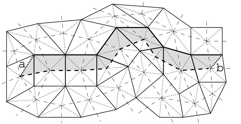
Figure 7: A ribbon on the lattice

The next task is to construct a set of operators which can create an arbitrary two-particle state from the ground state. I do not know how to deduce an expression for such operators; I will just give an answer and explain why it is correct. In the abelian case (see Sec. 2) there were two types of such operators which corresponded to paths on the lattice and the dual lattice, respectively. In the nonabelian case, we have to consider both types of paths together. Thus, the operators creating a particle pair are associated with a ribbon (see fig. 7). The ribbon connects two sites at which the particles will appear (say, $a=(s,p)$ and $b=(s^{\prime},p^{\prime})$). The corresponding operators act on the edges which constitute one side of the ribbon (solid line), as well as the edges intersected by the other side (dashed line).

For a given ribbon $t$, there are $N^{2}$ ribbon operators $F^{(h,g)}(t)$ indexed by $g,h\in G$. They act as follows

$$\begin{array}[]{rl}F^{(h,g)}(t)&\raisebox{-35.56593pt}{ \begin{picture}(3.0,1.2)\put(1.0,1.0){\vector(-1,0){1.0}} \put(0.0,1.0){\vbox{\hbox to71.13188pt{\hfil$x_{1}$\hfil} \kern 2.0pt}} \put(2.0,1.0){\vector(-1,0){1.0}} \put(1.0,1.0){\vbox{\hbox to71.13188pt{\hfil$x_{2}$\hfil} \kern 2.0pt}} \put(3.0,1.0){\vector(-1,0){1.0}} \put(2.0,1.0){\vbox{\hbox to71.13188pt{\hfil$x_{3}$\hfil} \kern 2.0pt}} \put(0.0,0.0){\vector(0,1){1.0}} \put(0.0,0.5){\kern 2.0pt$y_{1}$} \put(1.0,0.0){\vector(0,1){1.0}} \put(1.0,0.5){\kern 2.0pt$y_{2}$} \put(2.0,0.0){\vector(0,1){1.0}} \put(2.0,0.5){\kern 2.0pt$y_{3}$} \end{picture} }\qquad=\vskip 12.0pt plus 4.0pt minus 4.0pt\\ =\quad\delta_{g,\,x_{1}x_{2}x_{3}}&\raisebox{-35.56593pt}{ \begin{picture}(3.3,1.2)\put(1.0,1.0){\vector(-1,0){1.0}} \put(0.0,1.0){\vbox{\hbox to71.13188pt{\hfil$x_{1}$\hfil} \kern 2.0pt}} \put(2.0,1.0){\vector(-1,0){1.0}} \put(1.0,1.0){\vbox{\hbox to71.13188pt{\hfil$x_{2}$\hfil} \kern 2.0pt}} \put(3.0,1.0){\vector(-1,0){1.0}} \put(2.0,1.0){\vbox{\hbox to71.13188pt{\hfil$x_{3}$\hfil} \kern 2.0pt}} \put(0.0,0.0){\vector(0,1){1.0}} \put(0.0,0.5){\kern 2.0pt$hy_{1}$} \put(1.0,0.0){\vector(0,1){1.0}} \put(1.0,0.5){\kern 2.0pt$x_{1}^{-1}hx_{1}\,y_{2}$} \put(2.0,0.0){\vector(0,1){1.0}} \put(2.0,0.5){\kern 2.0pt$(x_{1}x_{2})^{-1}h(x_{1}x_{2})\,y_{3}$} \end{picture} }\end{array}$$ (24)

These operators commute with every projector $A(r)$, $B(l)$, except for $r=s,s^{\prime}$ and $l=p,p^{\prime}$. This is the first important property of ribbon operators.

The operators $F^{(h,g)}(t)$ depend on the ribbon $t$. However, their action on the space $\mathcal{L}(a,b)$ depends only on the topological class of the ribbon This is also true for a multi-particle excitation space $\mathcal{L}(x_{1},\ldots,x_{n})$. More exactly, consider two ribbons, $t$ and $q$, connecting the sites $x_{1}=a$ and $x_{2}=b$

The actions of $F^{(h,g)}(t)$ and $F^{(h,g)}(q)$ on $\mathcal{L}(x_{1},\ldots,x_{n})$ coincide provided none of the sites $x_{3},\ldots,x_{n}$ lie on or between the ribbons. This is the second important property of ribbon operators. We will write $F^{(h,g)}(t)\equiv F^{(h,g)}(q)$, or, more exactly, $F^{(h,g)}(t)\stackrel{{\scriptstyle M}}{{\equiv}}F^{(h,g)}(q)$, where $M=\{x_{1},\ldots,x_{n}\}$.

Linear combination of the operators $F^{(h,g)}(t)$ are also called ribbon operators. They form an algebra $\mathcal{F}(t)\cong\mathcal{F}$. The multiplication rules are as follows

$$F^{\mbox{\scriptsize\boldmath$m$}}(t)\,F^{\mbox{\scriptsize\boldmath$n$}}(t)\ =\ {\Lambda^{\mbox{\scriptsize\boldmath${m}{n}$}}_{\mbox{\scriptsize\boldmath$k$}}}\,F^{\mbox{\scriptsize\boldmath$k$}}(t)\qquad\qquad\Lambda^{(h_{1},g_{1})\,(h_{2},g_{2})}_{(h,g)}\ =\ \delta_{h_{1}h_{2},\,h}\ \delta_{g_{1},g}\ \delta_{g_{2},g}$$ (25)

(summation over $m$ and $n$ is implied).

Any ribbon operator on a long ribbon $t=t_{1}t_{2}$ (see figure below) can be represented in terms of ribbon operators corresponding to its parts, $t_{1}$ and $t_{2}$

$$F^{\mbox{\scriptsize\boldmath$k$}}(t_{1}t_{2})\ =\ {\Omega^{\mbox{\scriptsize\boldmath$k$}}_{\mbox{\scriptsize\boldmath$mn$}}}\,F^{\mbox{\scriptsize\boldmath$m$}}(t_{1})\,F^{\mbox{\scriptsize\boldmath$n$}}(t_{2})\qquad\qquad\Omega^{(h,g)}_{(h_{1},g_{1})\,(h_{2},g_{2})}\ =\ \delta_{g,\,g_{1}g_{2}}\ \delta_{h_{1},h}\ \delta_{h_{2},\,g_{1}^{-1}hg_{1}}$$ (26)

(Note that $F^{\mbox{\scriptsize\boldmath$m$}}(t_{1})$ and $F^{\mbox{\scriptsize\boldmath$n$}}(t_{2})$ commute because the ribbons $t_{1}$ and $t_{2}$ do ton overlap). By some miracle, the tensor $\Omega^{\star}_{\star\star}$ is the same as in eg. (18). From the mathematical point of view, eq. (26) defines a linear mapping  $\Delta(t_{1},t_{2}):\ \mathcal{F}(t_{1},t_{2})\to\mathcal{F}(t_{1})\otimes\mathcal{F}(t_{2})$,   or just $\Delta:\,\mathcal{F}\to\mathcal{F}$. Such a mapping is called a comultiplication.

The comultiplication rules (26) allow to give another definition of ribbon operators which is nicer than eq. (24). Note that a ribbon consists of triangles of two types (see fig. 7). Each triangle corresponds to one edge. More exactly, a triangle with two dotted sides and one dashed side corresponds to a combination of an edge and its endpoint, say, $i$ and $r$. Similarly, a triangle with a solid side corresponds to a combination of an edge and one of the adjacent faces, say, $j$ and $l$. Each triangle can be considered as a short ribbon. The corresponding ribbon operators are

$$F^{(h,g)}(i,r)\ =\ \delta_{g,1}\,L^{h}(i,r)\qquad\qquad\quad F^{(h,g)}(j,l)\ =\ T^{g^{-1}}(j,l)$$

The ribbon operators on a long ribbon can be constructed from these ones.

It has been already mentioned that the multiplication in $\mathcal{D}$ and the comultiplication in $\mathcal{F}$ are defined by the same tensor $\Omega^{\star}_{\star\star}$. Actually, $\mathcal{D}$ and $\mathcal{F}$ are Hopf algebras dual to each other. (For general account on Hopf algebras, see [21, 22, 23]). The multiplication in $\mathcal{F}$ corresponds to a comultiplication in $\mathcal{D}$ defined as follows

$$\Delta(D_{\mbox{\scriptsize\boldmath$k$}})\ =\ {\Lambda^{\mbox{\scriptsize\boldmath${m}{n}$}}_{\mbox{\scriptsize\boldmath$k$}}}\,D_{\mbox{\scriptsize\boldmath$m$}}\otimes D_{\mbox{\scriptsize\boldmath$n$}}$$ (27)

(More explicitly,   $\Delta(D_{(h,g)})\,=\,\sum_{h_{1}h_{2}=h}D_{(h_{1},g)}\otimes D_{(h_{2},g)}\$). The unit element of $\mathcal{F}$ is $1_{\mathcal{F}}=\mbox{\large$\varepsilon$}_{\mbox{\scriptsize\boldmath$k$}}F^{\mbox{\scriptsize\boldmath$k$}}$, where $\mbox{\large$\varepsilon$}_{\mbox{\scriptsize\boldmath$k$}}$ are given by eq. (21);  the tensor $\mbox{\large$\varepsilon$}_{\star}$ also defines a counit of $\mathcal{D}$ (i.e. the mapping $\mbox{\large$\varepsilon$}:\mathcal{D}\to\mathbb{C}$ :  $\mbox{\large$\varepsilon$}(D_{\mbox{\scriptsize\boldmath$k$}})=\mbox{\large$\varepsilon$}_{\mbox{\scriptsize\boldmath$k$}}$ ). The unit of $\mathcal{D}$ and the counit of $\mathcal{F}$ are given by

$$\mbox{\large$\mathrm{e}$}^{(h,g)}\ =\ \delta_{g,1}$$ (28)

The Hopf algebra structure also includes an antipode, i.e. a mapping $S:\mathcal{D}\to\mathcal{D}$ :  $S(D_{\mbox{\scriptsize\boldmath$k$}})={\mathrm{S}^{\mbox{\scriptsize\boldmath$m$}}_{\mbox{\scriptsize\boldmath$k$}}}D_{\mbox{\scriptsize\boldmath$m$}}$,  or $S:\mathcal{F}\to\mathcal{F}$ :  $S(F^{\mbox{\scriptsize\boldmath$m$}})={\mathrm{S}^{\mbox{\scriptsize\boldmath$m$}}_{\mbox{\scriptsize\boldmath$k$}}}F^{\mbox{\scriptsize\boldmath$k$}}$. The tensor $\mathrm{S}^{\star}_{\star}$ is given by the equation

$$\mathrm{S}^{(h_{1},g_{1})}_{(h_{2},g_{2})}\ =\ \delta_{g_{1}^{-1}h_{1}g_{1},\,h_{2}^{-1}}\ \delta_{g_{1},\,g_{2}^{-1}}$$ (29)

Here is the complete list of Hopf algebra axioms.

$${\Lambda^{\mbox{\scriptsize\boldmath${l}{m}$}}_{\mbox{\scriptsize\boldmath$i$}}}\ {\Lambda^{\mbox{\scriptsize\boldmath${i}{n}$}}_{\mbox{\scriptsize\boldmath$k$}}}\ =\ {\Lambda^{\mbox{\scriptsize\boldmath${l}{j}$}}_{\mbox{\scriptsize\boldmath$k$}}}\ {\Lambda^{\mbox{\scriptsize\boldmath${m}{n}$}}_{\mbox{\scriptsize\boldmath$j$}}}\qquad\qquad\qquad\mbox{\large$\varepsilon$}_{\mbox{\scriptsize\boldmath$i$}}\ {\Lambda^{\mbox{\scriptsize\boldmath${i}{m}$}}_{\mbox{\scriptsize\boldmath$k$}}}\ =\ {\Lambda^{\mbox{\scriptsize\boldmath${m}{j}$}}_{\mbox{\scriptsize\boldmath$k$}}}\ \mbox{\large$\varepsilon$}_{\mbox{\scriptsize\boldmath$j$}}\ =\ {\mbox{\large$\delta$}^{\mbox{\scriptsize\boldmath$m$}}_{\mbox{\scriptsize\boldmath$k$}}}$$ (30)

$${\Omega^{\mbox{\scriptsize\boldmath$i$}}_{\mbox{\scriptsize\boldmath$lm$}}}\ {\Omega^{\mbox{\scriptsize\boldmath$k$}}_{\mbox{\scriptsize\boldmath$in$}}}\ =\ {\Omega^{\mbox{\scriptsize\boldmath$k$}}_{\mbox{\scriptsize\boldmath$lj$}}}\ {\Omega^{\mbox{\scriptsize\boldmath$j$}}_{\mbox{\scriptsize\boldmath$mn$}}}\qquad\qquad\qquad\mbox{\large$\mathrm{e}$}^{\mbox{\scriptsize\boldmath$i$}}\ {\Omega^{\mbox{\scriptsize\boldmath$k$}}_{\mbox{\scriptsize\boldmath$in$}}}\ =\ {\Omega^{\mbox{\scriptsize\boldmath$k$}}_{\mbox{\scriptsize\boldmath$mj$}}}\ \mbox{\large$\mathrm{e}$}^{\mbox{\scriptsize\boldmath$j$}}\ =\ {\mbox{\large$\delta$}^{\mbox{\scriptsize\boldmath$k$}}_{\mbox{\scriptsize\boldmath$m$}}}$$ (31)

$${\Lambda^{\mbox{\scriptsize\boldmath${l}{m}$}}_{\mbox{\scriptsize\boldmath$q$}}}\ {\Omega^{\mbox{\scriptsize\boldmath$q$}}_{\mbox{\scriptsize\boldmath$kn$}}}\ =\ {\Omega^{\mbox{\scriptsize\boldmath$l$}}_{\mbox{\scriptsize\boldmath$ij$}}}\ {\Omega^{\mbox{\scriptsize\boldmath$m$}}_{\mbox{\scriptsize\boldmath$rs$}}}\ {\Lambda^{\mbox{\scriptsize\boldmath${i}{r}$}}_{\mbox{\scriptsize\boldmath$k$}}}\ {\Lambda^{\mbox{\scriptsize\boldmath${j}{s}$}}_{\mbox{\scriptsize\boldmath$n$}}}\qquad\qquad\mbox{\large$\varepsilon$}_{\mbox{\scriptsize\boldmath$q$}}\ {\Omega^{\mbox{\scriptsize\boldmath$q$}}_{\mbox{\scriptsize\boldmath$kn$}}}\ =\ \mbox{\large$\varepsilon$}_{\mbox{\scriptsize\boldmath$k$}}\,\mbox{\large$\varepsilon$}_{\mbox{\scriptsize\boldmath$n$}}\qquad\quad{\Lambda^{\mbox{\scriptsize\boldmath${l}{m}$}}_{\mbox{\scriptsize\boldmath$q$}}}\ \mbox{\large$\mathrm{e}$}^{\mbox{\scriptsize\boldmath$q$}}\ =\ \mbox{\large$\mathrm{e}$}^{\mbox{\scriptsize\boldmath$l$}}\,\mbox{\large$\mathrm{e}$}^{\mbox{\scriptsize\boldmath$m$}}$$ (32)

$${\mathrm{S}^{\mbox{\scriptsize\boldmath$k$}}_{\mbox{\scriptsize\boldmath$l$}}}\ {\Lambda^{\mbox{\scriptsize\boldmath${l}{m}$}}_{\mbox{\scriptsize\boldmath$p$}}}\ {\Omega^{\mbox{\scriptsize\boldmath$q$}}_{\mbox{\scriptsize\boldmath$kn$}}}\ {\mbox{\large$\delta$}^{\mbox{\scriptsize\boldmath$n$}}_{\mbox{\scriptsize\boldmath$m$}}}\ =\ {\mbox{\large$\delta$}^{\mbox{\scriptsize\boldmath$k$}}_{\mbox{\scriptsize\boldmath$l$}}}\ {\Lambda^{\mbox{\scriptsize\boldmath${l}{m}$}}_{\mbox{\scriptsize\boldmath$p$}}}\ {\Omega^{\mbox{\scriptsize\boldmath$q$}}_{\mbox{\scriptsize\boldmath$kn$}}}\ {\mathrm{S}^{\mbox{\scriptsize\boldmath$n$}}_{\mbox{\scriptsize\boldmath$m$}}}\ =\ \mbox{\large$\varepsilon$}_{\mbox{\scriptsize\boldmath$p$}}\,\mbox{\large$\mathrm{e}$}^{\mbox{\scriptsize\boldmath$q$}}$$ (33)

Most of these identities correspond to physically obvious properties of ribbon operators. Eq. (30) is a statement of the usual multiplication axioms in the algebra $\mathcal{F}$, namely,  $(F^{\mbox{\scriptsize\boldmath$l$}}F^{\mbox{\scriptsize\boldmath$m$}})F^{\mbox{\scriptsize\boldmath$n$}}=F^{\mbox{\scriptsize\boldmath$l$}}(F^{\mbox{\scriptsize\boldmath$m$}}F^{\mbox{\scriptsize\boldmath$n$}})$  and  $1F^{\mbox{\scriptsize\boldmath$m$}}=F^{\mbox{\scriptsize\boldmath$m$}}1=F^{\mbox{\scriptsize\boldmath$m$}}$. The first equation in (31) (coassociativity of the comultiplication in $\mathcal{F}$) can be proven by expanding $F^{\mbox{\scriptsize\boldmath$k$}}(t_{1}t_{2}t_{3})$ as  ${\Omega^{\mbox{\scriptsize\boldmath$k$}}_{\mbox{\scriptsize\boldmath$in$}}}\,F^{\mbox{\scriptsize\boldmath$i$}}(t_{1}t_{2})\,F^{\mbox{\scriptsize\boldmath$n$}}(t_{3})$  or  ${\Omega^{\mbox{\scriptsize\boldmath$k$}}_{\mbox{\scriptsize\boldmath$lj$}}}\,F^{\mbox{\scriptsize\boldmath$l$}}(t_{1})\,F^{\mbox{\scriptsize\boldmath$j$}}(t_{2}t_{3})$  — the result must be the same. Eqs. (32) mean that the multiplication and comultiplication are consistent with each other. To prove the first equation in (32), expand  $F^{\mbox{\scriptsize\boldmath$l$}}(t_{1}t_{2})\,F^{\mbox{\scriptsize\boldmath$m$}}(t_{1}t_{2})$  in two different ways. The second equation follows from the fact that $\mbox{\large$\varepsilon$}_{\mbox{\scriptsize\boldmath$q$}}\,F^{\mbox{\scriptsize\boldmath$q$}}(t_{1}t_{2})$ is the identity operator.

The antipode axiom (33) does not have explicit physical meaning. Mathematically, it is a definition of the tensor $\mathrm{S}^{\star}_{\star}$ :  the element $\mbox{\large$\gamma$}=\,{\mathrm{S}^{\mbox{\scriptsize\boldmath$l$}}_{\mbox{\scriptsize\boldmath$k$}}}\,F^{\mbox{\scriptsize\boldmath$k$}}\otimes D_{\mbox{\scriptsize\boldmath$l$}}\,\in\mathcal{F}\otimes\mathcal{D}$  is the inverse to the canonical element $\mbox{\large$\delta$}=F^{\mbox{\scriptsize\boldmath$i$}}\otimes D_{\mbox{\scriptsize\boldmath$i$}}$.  The antipode have the following properties which can be derived from (30–33)

$${\mathrm{S}^{\mbox{\scriptsize\boldmath$i$}}_{\mbox{\scriptsize\boldmath$l$}}}\ {\mathrm{S}^{\mbox{\scriptsize\boldmath$j$}}_{\mbox{\scriptsize\boldmath$m$}}}\ {\Lambda^{\mbox{\scriptsize\boldmath${l}{m}$}}_{\mbox{\scriptsize\boldmath$p$}}}\ =\ {\Lambda^{\mbox{\scriptsize\boldmath${j}{i}$}}_{\mbox{\scriptsize\boldmath$q$}}}\ {\mathrm{S}^{\mbox{\scriptsize\boldmath$q$}}_{\mbox{\scriptsize\boldmath$p$}}}\qquad\qquad\quad{\mathrm{S}^{\mbox{\scriptsize\boldmath$p$}}_{\mbox{\scriptsize\boldmath$q$}}}\ {\Omega^{\mbox{\scriptsize\boldmath$q$}}_{\mbox{\scriptsize\boldmath$ij$}}}\ =\ {\Omega^{\mbox{\scriptsize\boldmath$p$}}_{\mbox{\scriptsize\boldmath$ml$}}}\ {\mathrm{S}^{\mbox{\scriptsize\boldmath$m$}}_{\mbox{\scriptsize\boldmath$j$}}}\ {\mathrm{S}^{\mbox{\scriptsize\boldmath$l$}}_{\mbox{\scriptsize\boldmath$i$}}}$$ (34)

Finally, we can define a so-called skew antipode $\tilde{\mathrm{S}}^{\star}_{\star}$ as follows

$${\tilde{\mathrm{S}}^{\mbox{\scriptsize\boldmath$m$}}_{\mbox{\scriptsize\boldmath$i$}}}\ {\mathrm{S}^{\mbox{\scriptsize\boldmath$i$}}_{\mbox{\scriptsize\boldmath$n$}}}\ =\ {\mathrm{S}^{\mbox{\scriptsize\boldmath$m$}}_{\mbox{\scriptsize\boldmath$j$}}}\ {\tilde{\mathrm{S}}^{\mbox{\scriptsize\boldmath$j$}}_{\mbox{\scriptsize\boldmath$n$}}}\ =\ {\mbox{\large$\delta$}^{\mbox{\scriptsize\boldmath$m$}}_{\mbox{\scriptsize\boldmath$n$}}}$$ (35)

In our case, ${\tilde{\mathrm{S}}^{\mbox{\scriptsize\boldmath$m$}}_{\mbox{\scriptsize\boldmath$i$}}}={\mathrm{S}^{\mbox{\scriptsize\boldmath$m$}}_{\mbox{\scriptsize\boldmath$i$}}}$, but this is not true for a generic Hopf algebra. The skew antipode have the following properties similar to (33) and (34)

$${\tilde{\mathrm{S}}^{\mbox{\scriptsize\boldmath$n$}}_{\mbox{\scriptsize\boldmath$l$}}}\ {\Lambda^{\mbox{\scriptsize\boldmath${l}{m}$}}_{\mbox{\scriptsize\boldmath$p$}}}\ {\Omega^{\mbox{\scriptsize\boldmath$q$}}_{\mbox{\scriptsize\boldmath$kn$}}}\ {\mbox{\large$\delta$}^{\mbox{\scriptsize\boldmath$k$}}_{\mbox{\scriptsize\boldmath$m$}}}\ =\ {\mbox{\large$\delta$}^{\mbox{\scriptsize\boldmath$n$}}_{\mbox{\scriptsize\boldmath$l$}}}\ {\Lambda^{\mbox{\scriptsize\boldmath${l}{m}$}}_{\mbox{\scriptsize\boldmath$p$}}}\ {\Omega^{\mbox{\scriptsize\boldmath$q$}}_{\mbox{\scriptsize\boldmath$kn$}}}\ {\tilde{\mathrm{S}}^{\mbox{\scriptsize\boldmath$k$}}_{\mbox{\scriptsize\boldmath$m$}}}\ =\ \mbox{\large$\varepsilon$}_{\mbox{\scriptsize\boldmath$p$}}\,\mbox{\large$\mathrm{e}$}^{\mbox{\scriptsize\boldmath$q$}}$$ (36)

$${\tilde{\mathrm{S}}^{\mbox{\scriptsize\boldmath$i$}}_{\mbox{\scriptsize\boldmath$l$}}}\ {\tilde{\mathrm{S}}^{\mbox{\scriptsize\boldmath$j$}}_{\mbox{\scriptsize\boldmath$m$}}}\ {\Lambda^{\mbox{\scriptsize\boldmath${l}{m}$}}_{\mbox{\scriptsize\boldmath$p$}}}\ =\ {\Lambda^{\mbox{\scriptsize\boldmath${j}{i}$}}_{\mbox{\scriptsize\boldmath$q$}}}\ {\tilde{\mathrm{S}}^{\mbox{\scriptsize\boldmath$q$}}_{\mbox{\scriptsize\boldmath$p$}}}\qquad\qquad\quad{\tilde{\mathrm{S}}^{\mbox{\scriptsize\boldmath$p$}}_{\mbox{\scriptsize\boldmath$q$}}}\ {\Omega^{\mbox{\scriptsize\boldmath$q$}}_{\mbox{\scriptsize\boldmath$ij$}}}\ =\ {\Omega^{\mbox{\scriptsize\boldmath$p$}}_{\mbox{\scriptsize\boldmath$ml$}}}\ {\tilde{\mathrm{S}}^{\mbox{\scriptsize\boldmath$m$}}_{\mbox{\scriptsize\boldmath$j$}}}\ {\tilde{\mathrm{S}}^{\mbox{\scriptsize\boldmath$l$}}_{\mbox{\scriptsize\boldmath$i$}}}$$ (37)

(Note the distinction between (33) and (36), however).

The reader may be overwhelmed by a number of formal things, so let us summarize what we know by now. We have defined two algebras, $\mathcal{D}$ and $\mathcal{F}$, and their actions on the Hilbert space $\mathcal{N}$. In this context, we denote them by $\mathcal{D}(a)$ and $\mathcal{F}(t)$ because the actions depend on the site $a$ or on the ribbon $t$, respectively. Operators from $\mathcal{D}(a)$ affect one particle whereas operators from $\mathcal{F}(t)$ affect two particles. The action of $\mathcal{F}(t)$ on the space of $n$-particle states $\mathcal{L}(x_{1},\ldots,x_{n})$ depends only on the topological class of the ribbon $t$. This space have not been found yet, even for $n=2$. (It will be found after we learn more about local and ribbon operators). The algebra $\mathcal{F}$ is a Hopf algebra. The comultiplication allows to make up a long ribbon from parts. There is a formal duality between $\mathcal{F}$ and $\mathcal{D}$. The comultiplication in $\mathcal{F}$ is dual to the multiplication in $\mathcal{D}$. The multiplication in $\mathcal{F}$ is dual to a comultiplication in $\mathcal{D}$. (The meaning of the latter is not clear yet).

5.3 Further properties of local and ribbon operators

Figure 8: Two ribbons attached to the same site

Let us study commutation relations between ribbon operators. Consider two ribbons attached to the same site, as shown in fig. 8 a or b. Then

$$\begin{array}[]{rcl}F^{(h,g)}(t_{1})\ F^{(v,u)}(q_{1})&=&\,F^{(v,u)}(q_{1})\ F^{(v^{-1}hv,\,v^{-1}g)}(t_{1})\vskip 6.0pt plus 2.0pt minus 2.0pt\\ F^{(h,g)}(t_{2})\ F^{(v,u)}(q_{2})&=&\,F^{(v,u)}(q_{2})\ F^{(h,\,gu^{-1}vu)}(t_{2})\end{array}$$

In a tensor form, these equations read as follows

$$\begin{array}[]{rcl}F^{\mbox{\scriptsize\boldmath$m$}}(t_{1})\ F^{\mbox{\scriptsize\boldmath$n$}}(q_{1})&=&\,{\mathrm{R}^{\mbox{\scriptsize\boldmath$ik$}}}\ {\Omega^{\mbox{\scriptsize\boldmath$n$}}_{\mbox{\scriptsize\boldmath$ij$}}}\ {\Omega^{\mbox{\scriptsize\boldmath$m$}}_{\mbox{\scriptsize\boldmath$kl$}}}\ F^{\mbox{\scriptsize\boldmath$j$}}(q_{1})\ F^{\mbox{\scriptsize\boldmath$l$}}(t_{1})\vskip 12.0pt plus 4.0pt minus 4.0pt\\ F^{\mbox{\scriptsize\boldmath$m$}}(t_{2})\ F^{\mbox{\scriptsize\boldmath$n$}}(q_{2})&=&\,F^{\mbox{\scriptsize\boldmath$i$}}(q_{2})\ F^{\mbox{\scriptsize\boldmath$k$}}(t_{2})\ {\Omega^{\mbox{\scriptsize\boldmath$n$}}_{\mbox{\scriptsize\boldmath$ij$}}}\ {\Omega^{\mbox{\scriptsize\boldmath$m$}}_{\mbox{\scriptsize\boldmath$kl$}}}\ {\bar{\mathrm{R}}^{\mbox{\scriptsize\boldmath$jl$}}}\end{array}$$ (38)

where

$$\mathrm{R}^{(h,g)(v,u)}\ =\ \delta_{h,u}\ \delta_{g,1}\qquad\qquad\quad\bar{\mathrm{R}}^{(h,g)(v,u)}\ =\ \delta_{h^{-1}\!,\,u}\ \delta_{g,1}$$ (39)

Note that

$${\bar{\mathrm{R}}^{\mbox{\scriptsize\boldmath$ik$}}}\ {\Omega^{\mbox{\scriptsize\boldmath$n$}}_{\mbox{\scriptsize\boldmath$ij$}}}\ {\Omega^{\mbox{\scriptsize\boldmath$m$}}_{\mbox{\scriptsize\boldmath$kl$}}}\ {\mathrm{R}^{\mbox{\scriptsize\boldmath$jl$}}}\,\ =\,\ {\mathrm{R}^{\mbox{\scriptsize\boldmath$ik$}}}\ {\Omega^{\mbox{\scriptsize\boldmath$n$}}_{\mbox{\scriptsize\boldmath$ij$}}}\ {\Omega^{\mbox{\scriptsize\boldmath$m$}}_{\mbox{\scriptsize\boldmath$kl$}}}\ {\bar{\mathrm{R}}^{\mbox{\scriptsize\boldmath$jl$}}}\,\ =\,\ \mbox{\large$\mathrm{e}$}^{\mbox{\scriptsize\boldmath$n$}}\,\mbox{\large$\mathrm{e}$}^{\mbox{\scriptsize\boldmath$m$}}$$ (40)

To prove (and to see the physical meaning of) this equation, consider the configuration shown in fig. 9b. Clearly, $F^{\mbox{\scriptsize\boldmath$r$}}(t_{2}t_{1})$ and $F^{\mbox{\scriptsize\boldmath$s$}}(q^{\prime})$ commute. On the other hand, $F^{\mbox{\scriptsize\boldmath$s$}}(q^{\prime})\equiv F^{\mbox{\scriptsize\boldmath$s$}}(q_{2}q_{1})$, so $F^{\mbox{\scriptsize\boldmath$r$}}(t_{2}t_{1})$ and $F^{\mbox{\scriptsize\boldmath$s$}}(q_{2}q_{1})$ commute. It follows that  ${\bar{\mathrm{R}}^{\mbox{\scriptsize\boldmath$ik$}}}\,{\Omega^{\mbox{\scriptsize\boldmath$n$}}_{\mbox{\scriptsize\boldmath$ij$}}}\,{\Omega^{\mbox{\scriptsize\boldmath$m$}}_{\mbox{\scriptsize\boldmath$kl$}}}\,{\mathrm{R}^{\mbox{\scriptsize\boldmath$jl$}}}\,=\,\mbox{\large$\mathrm{e}$}^{\mbox{\scriptsize\boldmath$n$}}\mbox{\large$\mathrm{e}$}^{\mbox{\scriptsize\boldmath$m$}}$.  This identity can be easily written in an invariant form, namely, $\bar{R}R=1_{\mathcal{D}\otimes\mathcal{D}}$,  where $R={\mathrm{R}^{\mbox{\scriptsize\boldmath$jl$}}}\,D_{\mbox{\scriptsize\boldmath$j$}}\otimes D_{\mbox{\scriptsize\boldmath$l$}}$  and $\bar{R}={\bar{\mathrm{R}}^{\mbox{\scriptsize\boldmath$ik$}}}\,D_{\mbox{\scriptsize\boldmath$i$}}\otimes D_{\mbox{\scriptsize\boldmath$k$}}$. It also implies that $R\bar{R}=1_{\mathcal{D}\otimes\mathcal{D}}$ because the algebra $\mathcal{D}\otimes\mathcal{D}$ is finite dimensional. Thus, $\bar{R}=R^{-1}$.

Figure 9: Checking consistency of the commutation relations

The tensor $\mathrm{R}^{\star}_{\star}$ (or the element $R\in\mathcal{D}\otimes\mathcal{D}$) is called the $R$-matrix. It satisfies the following axioms

$${\Lambda^{\mbox{\scriptsize\boldmath${i}{j}$}}_{\mbox{\scriptsize\boldmath$k$}}}\ {\mathrm{R}^{\mbox{\scriptsize\boldmath$km$}}}\ =\ {\mathrm{R}^{\mbox{\scriptsize\boldmath$il$}}}\ {\mathrm{R}^{\mbox{\scriptsize\boldmath$jn$}}}\ {\Omega^{\mbox{\scriptsize\boldmath$m$}}_{\mbox{\scriptsize\boldmath$ln$}}}\qquad\qquad\qquad{\mathrm{R}^{\mbox{\scriptsize\boldmath$mk$}}}{\Lambda^{\mbox{\scriptsize\boldmath${j}{i}$}}_{\mbox{\scriptsize\boldmath$k$}}}\ =\ {\Omega^{\mbox{\scriptsize\boldmath$m$}}_{\mbox{\scriptsize\boldmath$ln$}}}\ {\mathrm{R}^{\mbox{\scriptsize\boldmath$li$}}}\ {\mathrm{R}^{\mbox{\scriptsize\boldmath$nj$}}}$$ (41)

$${\Lambda^{\mbox{\scriptsize\boldmath${j}{i}$}}_{\mbox{\scriptsize\boldmath$k$}}}\ =\ {\Omega^{\mbox{\scriptsize\boldmath$i$}}_{\mbox{\scriptsize\boldmath$lmr$}}}\ {\Omega^{\mbox{\scriptsize\boldmath$j$}}_{\mbox{\scriptsize\boldmath$pns$}}}\ {\mathrm{R}^{\mbox{\scriptsize\boldmath$lp$}}}\ {\Lambda^{\mbox{\scriptsize\boldmath${m}{n}$}}_{\mbox{\scriptsize\boldmath$k$}}}\ {\bar{\mathrm{R}}^{\mbox{\scriptsize\boldmath$rs$}}}$$ (42)

where ${\Omega^{\mbox{\scriptsize\boldmath$i$}}_{\mbox{\scriptsize\boldmath$lmr$}}}={\Omega^{\mbox{\scriptsize\boldmath$i$}}_{\mbox{\scriptsize\boldmath$lu$}}}{\Omega^{\mbox{\scriptsize\boldmath$u$}}_{\mbox{\scriptsize\boldmath$mr$}}}={\Omega^{\mbox{\scriptsize\boldmath$u$}}_{\mbox{\scriptsize\boldmath$lm$}}}{\Omega^{\mbox{\scriptsize\boldmath$i$}}_{\mbox{\scriptsize\boldmath$ur$}}}$. Eqs. (41) follow from (38). Conversely, these equations ensure that the commutation relation are consistent. To prove the first equation in (41), commute $F^{\mbox{\scriptsize\boldmath$m$}}(t_{1})\,F^{\mbox{\scriptsize\boldmath$i$}}(q_{1})\,F^{\mbox{\scriptsize\boldmath$j$}}(q_{1})$ in two different ways. You will get $\mathrm{W}^{\mbox{\scriptsize\boldmath$ijm$}}_{\mbox{\scriptsize\boldmath$ab$}}\,F^{\mbox{\scriptsize\boldmath$a$}}(q_{1})\,F^{\mbox{\scriptsize\boldmath$b$}}(t_{1})$, with two different expressions for $\mathrm{W}^{\mbox{\scriptsize\boldmath$ijm$}}_{\mbox{\scriptsize\boldmath$ab$}}$. Then calculate $\mathrm{W}^{\mbox{\scriptsize\boldmath$ijm$}}_{\mbox{\scriptsize\boldmath$ab$}}\,\mbox{\large$\mathrm{e}$}^{\mbox{\scriptsize\boldmath$a$}}\,\mbox{\large$\mathrm{e}$}^{\mbox{\scriptsize\boldmath$b$}}$  using the axioms (30–32). The second equation in (41) can be proven in a similar way.

To prove eq. (42), consider the configuration shown in fig. 9a. Clearly, $F^{\mbox{\scriptsize\boldmath$i$}}(q_{1}q_{2})\equiv F^{\mbox{\scriptsize\boldmath$i$}}(t_{1}t_{2})$,  so  $F^{\mbox{\scriptsize\boldmath$j$}}(t_{1}t_{2})\,F^{\mbox{\scriptsize\boldmath$i$}}(q_{1}q_{2})\,\equiv\,{\Lambda^{\mbox{\scriptsize\boldmath${j}{i}$}}_{\mbox{\scriptsize\boldmath$k$}}}\,F^{\mbox{\scriptsize\boldmath$k$}}(t_{1}t_{2})$.  On the other hand, we can first expand $F^{\mbox{\scriptsize\boldmath$j$}}(t_{1}t_{2})$ and $F^{\mbox{\scriptsize\boldmath$i$}}(q_{1}q_{2})$ using the comultiplication rules, and then apply the commutation relations (38). The result must be the same.

Let $t$ be a ribbon connecting sites $a$ and $b$. The local and ribbon operators commute as follows

$$F^{\mbox{\scriptsize\boldmath$m$}}(t)\ D_{\mbox{\scriptsize\boldmath$i$}}(a)\ =\ {\Lambda^{\mbox{\scriptsize\boldmath${j}{k}$}}_{\mbox{\scriptsize\boldmath$i$}}}\ {\Omega^{\mbox{\scriptsize\boldmath$m$}}_{\mbox{\scriptsize\boldmath$kl$}}}\ D_{\mbox{\scriptsize\boldmath$j$}}(a)\ F^{\mbox{\scriptsize\boldmath$l$}}(t)\qquad\qquad D_{\mbox{\scriptsize\boldmath$i$}}(b)\ F^{\mbox{\scriptsize\boldmath$m$}}(t)\ =\ {\Omega^{\mbox{\scriptsize\boldmath$m$}}_{\mbox{\scriptsize\boldmath$lk$}}}\ {\Lambda^{\mbox{\scriptsize\boldmath${k}{j}$}}_{\mbox{\scriptsize\boldmath$i$}}}\ F^{\mbox{\scriptsize\boldmath$l$}}(t)\ D_{\mbox{\scriptsize\boldmath$j$}}(b)$$ (43)

These commutation relations can be also written in the form

$$\begin{array}[]{rcl}D_{\mbox{\scriptsize\boldmath$j$}}(a)\ F^{\mbox{\scriptsize\boldmath$l$}}(t)&\,=&{\Lambda^{\mbox{\scriptsize\boldmath${i}{k}$}}_{\mbox{\scriptsize\boldmath$j$}}}\ {\tilde{\mathrm{S}}^{\mbox{\scriptsize\boldmath$n$}}_{\mbox{\scriptsize\boldmath$k$}}}\ {\Omega^{\mbox{\scriptsize\boldmath$l$}}_{\mbox{\scriptsize\boldmath$nm$}}}\ F^{\mbox{\scriptsize\boldmath$m$}}(t)\ D_{\mbox{\scriptsize\boldmath$i$}}(a)\vskip 6.0pt plus 2.0pt minus 2.0pt\\ F^{\mbox{\scriptsize\boldmath$l$}}(t)\ D_{\mbox{\scriptsize\boldmath$j$}}(b)&\,=&{\Omega^{\mbox{\scriptsize\boldmath$l$}}_{\mbox{\scriptsize\boldmath$mn$}}}\ {\tilde{\mathrm{S}}^{\mbox{\scriptsize\boldmath$n$}}_{\mbox{\scriptsize\boldmath$k$}}}\ {\Lambda^{\mbox{\scriptsize\boldmath${k}{i}$}}_{\mbox{\scriptsize\boldmath$j$}}}\ D_{\mbox{\scriptsize\boldmath$i$}}(b)\ F^{\mbox{\scriptsize\boldmath$m$}}(t)\end{array}$$ (44)

where $\tilde{\mathrm{S}}^{\star}_{\star}$ is the skew antipode (see eqs. (35,36)).

Finally, we introduce some special elements $C\in\mathcal{D}$ and $\mbox{\large$\tau$}\in\mathcal{F}$. The first one has a clear physical meaning:  the corresponding operator $C(a)=A(a)\,B(a)$ projects out states with no particle at the site $a$. The element $C$ can be represented in the form

$$C\ =\ \mbox{\large$\mathrm{c}$}^{\mbox{\scriptsize\boldmath$i$}}\,D_{\mbox{\scriptsize\boldmath$i$}}\qquad\qquad\mbox{where}\quad\mbox{\large$\mathrm{c}$}^{(h,g)}\,=\,N^{-1}\delta_{h,1}$$ (45)

It has the following properties:

$$CX\,=\ XC\,=\,\mbox{\large$\varepsilon$}(X)\,C\quad\mbox{for any}\,\ X\in\mathcal{D}\,\qquad\qquad\qquad\mbox{\large$\varepsilon$}(C)\,=\,1$$

or, in tensor notations,

$${\Omega^{\mbox{\scriptsize\boldmath$k$}}_{\mbox{\scriptsize\boldmath$ij$}}}\,\mbox{\large$\mathrm{c}$}^{\mbox{\scriptsize\boldmath$i$}}\ =\ {\Omega^{\mbox{\scriptsize\boldmath$k$}}_{\mbox{\scriptsize\boldmath$ji$}}}\,\mbox{\large$\mathrm{c}$}^{\mbox{\scriptsize\boldmath$i$}}\ =\ \mbox{\large$\varepsilon$}_{\mbox{\scriptsize\boldmath$j$}}\,\mbox{\large$\mathrm{c}$}^{\mbox{\scriptsize\boldmath$k$}}\qquad\qquad\qquad\mbox{\large$\varepsilon$}_{\mbox{\scriptsize\boldmath$k$}}\,\mbox{\large$\mathrm{c}$}^{\mbox{\scriptsize\boldmath$k$}}\ =\ 1$$ (46)

The element $\mbox{\large$\tau$}\in\mathcal{F}$ is dual to $C$; it is defined as follows

$$\mbox{\large$\tau$}\ =\ \mbox{\large$\tau$}_{\mbox{\scriptsize\boldmath$i$}}\,F^{\mbox{\scriptsize\boldmath$i$}}\qquad\qquad\mbox{where}\quad\mbox{\large$\tau$}_{(h,g)}\,=\,N^{-1}\delta_{1,g}$$ (47)

Its properties are as follows

$${\Lambda^{\mbox{\scriptsize\boldmath${i}{j}$}}_{\mbox{\scriptsize\boldmath$k$}}}\,\mbox{\large$\tau$}_{\mbox{\scriptsize\boldmath$i$}}\ =\ {\Lambda^{\mbox{\scriptsize\boldmath${j}{i}$}}_{\mbox{\scriptsize\boldmath$k$}}}\,\mbox{\large$\tau$}_{\mbox{\scriptsize\boldmath$i$}}\ =\ \mbox{\large$\mathrm{e}$}^{\mbox{\scriptsize\boldmath$j$}}\,\mbox{\large$\tau$}_{\mbox{\scriptsize\boldmath$k$}}\qquad\qquad\qquad\mbox{\large$\mathrm{e}$}^{\mbox{\scriptsize\boldmath$k$}}\,\mbox{\large$\tau$}_{\mbox{\scriptsize\boldmath$k$}}\ =\ 1$$ (48)

Note that $\mbox{\large$\tau$}_{\mbox{\scriptsize\boldmath$k$}}\,\mbox{\large$\mathrm{c}$}^{\mbox{\scriptsize\boldmath$k$}}=N^{-2}$. Using these properties, we can we can derive an important consequence from the commutation relations (43)

$$\mbox{\large$\tau$}_{\mbox{\scriptsize\boldmath$s$}}\,{\Omega^{\mbox{\scriptsize\boldmath$s$}}_{\mbox{\scriptsize\boldmath$mp$}}}\,{\mathrm{S}^{\mbox{\scriptsize\boldmath$p$}}_{\mbox{\scriptsize\boldmath$q$}}}\ F^{\mbox{\scriptsize\boldmath$m$}}(t)\,C(a)\,F^{\mbox{\scriptsize\boldmath$q$}}(t)\,\ =\,\ \mbox{\large$\tau$}_{\mbox{\scriptsize\boldmath$s$}}\,{\Omega^{\mbox{\scriptsize\boldmath$s$}}_{\mbox{\scriptsize\boldmath$pm$}}}\,{\mathrm{S}^{\mbox{\scriptsize\boldmath$p$}}_{\mbox{\scriptsize\boldmath$q$}}}\ F^{\mbox{\scriptsize\boldmath$q$}}(t)\,C(b)\,F^{\mbox{\scriptsize\boldmath$m$}}(t)\,\ =\,\ N^{-2}$$ (49)

5.4 The space $\mathcal{L}(a,b)$

Now we are in a position to find the space $\mathcal{L}(a,b)$ and to prove the assertions from Sec. 5.1. The first assertion was that any excited spot can be transformed into one particle. It is simple if we can transform two particles into one by ribbon operators. Let us choose an arbitrary site $b$ the excited spot to be compressed to. Let some constraint, $A(s)-1\equiv 0$ or $B(p)-1\equiv 0$, be violated. Choose any site $a$ containing the vertex $s$ or the face $p$. Connect $a$ and $b$ by a ribbon. By the assumption, we can clean up the site $a$ while changing the state of $b$, but without violating any more constraint. We can repeat this procedure again and again to clean up the whole spot.

So, we only need to show that two particles can be transformed into one. What does it mean exactly? Physically, any transformation must be unitary, but it can involve also some external system. (Otherwise, it is impossible to “decrease entropy”, i.e. to convert many states into fewer). On the other hand, it is clear that unitarity is not relevant to this problem. However, we should exclude degenerate transformations, such as multiplication by the zero operator. So, it is better to reformulate the assertion as follows:  any two-particle state (plus some other excitations far away) can be obtained from one-particle states (plus the same excitations far away). Let $|\psi\rangle\in\mathcal{L}(a,b,\ldots)$ be such a two-particle state. We are going to use the formula (49). Let

$$G_{\mbox{\scriptsize\boldmath$q$}}\ =\ N^{2}\,\mbox{\large$\tau$}_{\mbox{\scriptsize\boldmath$s$}}\,{\Omega^{\mbox{\scriptsize\boldmath$s$}}_{\mbox{\scriptsize\boldmath$mp$}}}\,{\mathrm{S}^{\mbox{\scriptsize\boldmath$p$}}_{\mbox{\scriptsize\boldmath$q$}}}\ F^{\mbox{\scriptsize\boldmath$m$}}(t)\qquad\qquad\quad|\eta^{\mbox{\scriptsize\boldmath$q$}}\rangle\ =\ C(a)\,F^{\mbox{\scriptsize\boldmath$q$}}(t)\,|\psi\rangle$$ (50)

Then  $|\psi\rangle\,=\,G_{\mbox{\scriptsize\boldmath$q$}}\,|\eta^{\mbox{\scriptsize\boldmath$q$}}\rangle$. The states $|\eta^{\mbox{\scriptsize\boldmath$q$}}\rangle$ belong to $\mathcal{L}(b,\ldots)$, i.e. do not contain excitation at $a$. This is exactly what we need.

The other two assertions were about the action of local operators on the space $\mathcal{L}(a,b)$, so we need to find this space first. We can consider this space as a representation of the algebra $\mathcal{E}\cong\mathcal{E}(t)$ generated by the operators  $D_{\mbox{\scriptsize\boldmath$j$}}=D_{\mbox{\scriptsize\boldmath$j$}}(a)$,   $F^{\mbox{\scriptsize\boldmath$l$}}=F^{\mbox{\scriptsize\boldmath$l$}}(t)$  and $D_{\mbox{\scriptsize\boldmath$j$}}^{\prime}=D_{\mbox{\scriptsize\boldmath$j$}}(b)$. As a linear space, $\mathcal{E}=\mathcal{D}\otimes\mathcal{F}\otimes\mathcal{D}$. (Thus, $\mathcal{E}$ has dimensionality $N^{6}$). Multiplication in $\mathcal{E}$ is defined by the commutation relations (43). We will call $\mathcal{E}\cong\mathcal{E}(t)$ the algebra of extended ribbon operators. It is just an algebra, not a Hopf algebra. More exactly, it is a finite-dimensional $C^{*}$-algebra. The involution ($=$Hermitian conjugation) is given by the formulas (cf. (19))

$$(D_{(h,g)})^{\dagger}\ =\ D_{(g^{-1}hg,\,g^{-1})}\qquad\quad(F^{(h,g)})^{\dagger}\ =\ F^{(h^{-1},g)}\qquad\quad(D^{\prime}_{(h,g)})^{\dagger}\ =\ D^{\prime}_{(g^{-1}hg,\,g^{-1})}$$ (51)

[Remark.  Apparently, the algebra $\mathcal{E}$ will play the central role in a general theory of topological quantum order. Indeed, we were lucky to define ribbon operators separately from local operators. In the general case, ribbon operators should be mixed with local operators.]

So, we are looking for a particular representation $\mathcal{L}$ of the algebra $\mathcal{E}$. This representation must contain a special vector $|\xi\rangle$ (the ground state) such that

$$D_{\mbox{\scriptsize\boldmath$k$}}\,|\xi\rangle\ =\ \mbox{\large$\varepsilon$}_{\mbox{\scriptsize\boldmath$k$}}\,|\xi\rangle\qquad\qquad\quad D_{\mbox{\scriptsize\boldmath$k$}}^{\prime}\,|\xi\rangle\ =\ \mbox{\large$\varepsilon$}_{\mbox{\scriptsize\boldmath$k$}}\,|\xi\rangle$$ (52)

We start with constructing a representation $\check{\mathcal{L}}$ spanned by the vectors $|\psi^{\mbox{\scriptsize\boldmath$k$}}\rangle\,=\,F^{\mbox{\scriptsize\boldmath$k$}}\,|\xi\rangle$. (It will be proven after that $\check{\mathcal{L}}=\mathcal{L}$). We assume that the vectors $|\psi^{\mbox{\scriptsize\boldmath$k$}}\rangle$ are linearly independent. This need not be the case in the representation $\mathcal{L}$ but we can postulate $|\psi^{\mbox{\scriptsize\boldmath$k$}}\rangle$ being linearly independent in $\check{\mathcal{L}}$. Thus, $\mathcal{L}$ contains a factor-representation of $\check{\mathcal{L}}$.

The representation $\check{\mathcal{L}}$ is given by the formulas

$$D_{\mbox{\scriptsize\boldmath$j$}}\,|\psi^{\mbox{\scriptsize\boldmath$k$}}\rangle\ =\ {\tilde{\mathrm{S}}^{\mbox{\scriptsize\boldmath$n$}}_{\mbox{\scriptsize\boldmath$j$}}}\,{\Omega^{\mbox{\scriptsize\boldmath$k$}}_{\mbox{\scriptsize\boldmath$nm$}}}\,|\psi^{\mbox{\scriptsize\boldmath$m$}}\rangle\qquad\quad F^{\mbox{\scriptsize\boldmath$j$}}\,|\psi^{\mbox{\scriptsize\boldmath$k$}}\rangle\ =\ {\Lambda^{\mbox{\scriptsize\boldmath${j}{k}$}}_{\mbox{\scriptsize\boldmath$m$}}}\,|\psi^{\mbox{\scriptsize\boldmath$m$}}\rangle\qquad\quad D_{\mbox{\scriptsize\boldmath$j$}}^{\prime}\,|\psi^{\mbox{\scriptsize\boldmath$k$}}\rangle\ =\ {\Omega^{\mbox{\scriptsize\boldmath$k$}}_{\mbox{\scriptsize\boldmath$mj$}}}\,|\psi^{\mbox{\scriptsize\boldmath$m$}}\rangle$$ (53)

It is easy to show that this representation is irreducible. Hence, $\mathcal{L}$ contains $\check{\mathcal{L}}$, i.e. the vectors $|\psi^{\mbox{\scriptsize\boldmath$k$}}\rangle$ are linearly independent in $\mathcal{L}$. The scalar products between the vectors $|\psi^{\mbox{\scriptsize\boldmath$k$}}\rangle$ can be found from (53) and (51),

$$\langle\psi^{(v,u)}|\psi^{(h,g)}\rangle\ =\ N^{-1}\,\delta_{v,h}\,\delta_{u,g}$$ (54)

To prove that $\check{\mathcal{L}}=\mathcal{L}$, we use the equation (49) again. For an arbitrary two-particle state $|\psi\rangle\in\mathcal{L}$, define the vectors $|\eta^{\mbox{\scriptsize\boldmath$q$}}\rangle$ and operators $G_{\mbox{\scriptsize\boldmath$q$}}$ as in eq. (50). Then $|\psi\rangle\,=\,G_{\mbox{\scriptsize\boldmath$q$}}\,|\eta^{\mbox{\scriptsize\boldmath$q$}}\rangle$. One could say that $|\eta^{\mbox{\scriptsize\boldmath$q$}}\rangle\in\mathcal{L}(b)$ but, actually, the space $\mathcal{L}(b)$ is spanned by the sole vector $|\xi\rangle$. It follows that $|\psi\rangle\in\check{\mathcal{L}}$  — the assertion has been proven. Thus, the action of local and ribbon operators on the space $\mathcal{L}=\mathcal{L}(a,b)$ is given by eq. (53).

It is easy to see that the action of $\mathcal{D}(a)$ on $\mathcal{L}(a,b)$ is exact (though it is reducible). Besides that, $\mathcal{D}(a)$ is the commutant of $\mathcal{D}(b)$ in $\mathbf{L}(\mathcal{L}(a,b))$ and vise versa. (That is, $\mathcal{D}(a)$ consists of all operators $X\in\mathbf{L}(\mathcal{L}(a,b))$ which commute with every $Y\in\mathcal{D}(b)\,$). Hence, $\mathcal{D}(a)$ includes all local operators acting on the space $\mathcal{L}(a,b)$. Indeed, a local operator, which involves only spins near the site $a$, must commute with any operator acting on distant spins. Of course, there are many such operators, but their action on the two-particle space $\mathcal{L}(a,b)$ coincides with the action of the operators from $\mathcal{D}(a)$. This is also true for a multi-particle excitation space $\mathcal{L}(x_{1},\ldots,x_{n})$.

The space $\mathcal{L}(x_{1},\ldots,x_{n})$ can be described as follows. Let us connect the sites $x_{1},\ldots,x_{n}$ by $n-1$ ribbons $t_{1},\ldots,t_{n-1}$ in an arbitrary way so that the ribbons form a tree. Then the vectors $|\psi^{\mbox{\scriptsize\boldmath$k_{1},\ldots,k_{n-1}$}}\rangle\,=\,F^{\mbox{\scriptsize\boldmath$k_{1}$}}(t_{1})\ldots F^{\mbox{\scriptsize\boldmath$k_{n-1}$}}(t_{n-1})\,|\xi\rangle$ form a basis of $\mathcal{L}(x_{1},\ldots,x_{n})$. Choosing different ribbons means choosing a different basis. In the next section we will give another description of multi-particle excitation spaces.

6 Topological operators, braiding and fusion

Let us consider again the $n$-particle excitation space $\mathcal{L}=\mathcal{L}(x_{1},\ldots,x_{n})$. The algebra $\mathbf{L}(\mathcal{L})$ includes the local operator algebras $\mathcal{D}(x_{1}),\ldots,\mathcal{D}(x_{1})$. An operator $Y\in\mathbf{L}(\mathcal{L})$ which commute with every $X\in\mathcal{D}(x_{j})$   ($j=1,\ldots,n$)   is called a topological operator. Physically, topological operators correspond to nonlocal degrees of freedom. For $n=2$, the algebra of topological operators coincides with the center of $\mathcal{D}(x_{1})$ or $\mathcal{D}(x_{2})$. (The two centers coincide). Hence, the only nonlocal degree of freedom is the type of either particle. (The two particles correspond to dual representations of $\mathcal{D}$; in other words, these are a particle and an anti-particle). So, there is no hidden (i.e. quantum nonlocal) degree of freedom in this case. Such hidden degrees of freedom appear for $n\geq 3$.

To describe the space $\mathcal{L}$ and operators acting on it, let us choose an arbitrary site $x_{0}$ (distinct from $x_{1},\ldots,x_{n}$) and connect it with $x_{1},\ldots,x_{n}$ by non-intersecting ribbons $t_{1},\ldots,t_{n}$, see fig. 10a. As stated above, the space $\mathcal{L}(x_{0},x_{1},\ldots,x_{n})$ is spanned by the vectors

$$|\psi^{\mbox{\scriptsize\boldmath$k_{1},\ldots,k_{n}$}}\rangle\ =\ F^{\mbox{\scriptsize\boldmath$k_{1}$}}(t_{1})\ldots F^{\mbox{\scriptsize\boldmath$k_{n}$}}(t_{n})\,|\xi\rangle$$ (55)

The space in question, $\mathcal{L}=\mathcal{L}(x_{1},\ldots,x_{n})$ is contained in $\mathcal{L}(x_{0},x_{1},\ldots,x_{n})$. It consists of all vectors $|\psi\rangle\in\mathcal{L}(x_{0},x_{1},\ldots,x_{n})$ which are invariant under the action of $\mathcal{D}(x_{0})$ on the latter space.

The advantage of this description is that we can easily find all operators on the space $\mathcal{L}(x_{0},x_{1},\ldots,x_{n})$ which commute with $\mathcal{D}(x_{1})\otimes\ldots\otimes\mathcal{D}(x_{n})$. These are simply operators which act on the ends of the ribbons $t_{1},\ldots,t_{n}$ attached to the site $x_{0}$. More exactly, an operator $D_{\mbox{\scriptsize\boldmath$j$}}^{(r)}$   $(r=1,\ldots,n)$  acts on the $r$-th ribbon as $D_{\mbox{\scriptsize\boldmath$j$}}^{\prime}=D_{\mbox{\scriptsize\boldmath$j$}}(x_{0})$ (see eq.(53)), but does not affect the other ribbons,

$$\Bigl{(}D_{\mbox{\scriptsize\boldmath$j_{1}$}}^{(1)}\otimes\ldots\otimes D_{\mbox{\scriptsize\boldmath$j_{n}$}}^{(n)}\Bigr{)}\ |\psi^{\mbox{\scriptsize\boldmath$k_{1},\ldots,k_{n}$}}\rangle\,\ =\,\ {\Omega^{\mbox{\scriptsize\boldmath$k_{1}$}}_{\mbox{\scriptsize\boldmath$m_{1}j_{1}$}}}\ldots{\Omega^{\mbox{\scriptsize\boldmath$k_{n}$}}_{\mbox{\scriptsize\boldmath$m_{n}j_{n}$}}}\,|\psi^{\mbox{\scriptsize\boldmath$m_{1},\ldots,m_{n}$}}\rangle$$ (56)

Thus we arrive to an interesting physical conclusion. Let us consider only one particle attached to an end of a semi-infinite ribbon (an analog of Dirac’s string). Then the topological operators act on the far end of the ribbon.

Example.  Let us see how the topological operators act on magnetic vortices. As shown in Sec. 5.1, a vortex type is characterized by a conjugacy class $C$ of the group $G$. Individual topological states of the particle are characterized by particular elements $v\in C$. In terms of the notation (55), such a state can be represented as follows

$$|u,v\rangle\ =\ |C|^{1/2}\sum_{x:\ x^{-1}ux=v}\,|\psi^{(u,x)}\rangle$$

where $u\in C$ characterize the local state of the particle. One can easily check that $D_{(h,g)}^{\prime}|u,v\rangle\,=\,\delta_{h,\,gvg^{-1}}|u,h\rangle$. This is consistent with eq. (22). Note that the local degree of freedom, $u$, is not affected.

Figure 10: Braiding and fusion in terms of ribbon transformations

How can we physically apply topological operators to particles? We can just move the particles around each other; this process is called braiding. Let us see what happens if we interchange two particles, $x_{s}$ and $x_{s+1}$, counterclockwise, as shown in fig. 10b. The state $|\psi^{\mbox{\scriptsize\boldmath$\ldots,k,l,\ldots$}}\rangle$ becomes a new state

$$|\psi^{\mbox{\scriptsize\boldmath$\ldots,k,l,\ldots$}}\rangle_{\raisebox{-0.90417pt}{\scriptsize new}}\,\ =\,\ \mathcal{R}_{\curvearrowleft}\,|\psi^{\mbox{\scriptsize\boldmath$\ldots,k,l,\ldots$}}\rangle\,\ =\,\ \ldots F^{\mbox{\scriptsize\boldmath$k$}}(t^{\prime}_{s})\ F^{\mbox{\scriptsize\boldmath$l$}}(t^{\prime}_{s+1})\ldots\,|\xi\rangle$$

To represent this state in the old basis, we should represent the operator $F^{\mbox{\scriptsize\boldmath$k$}}(t^{\prime}_{s})\,F^{\mbox{\scriptsize\boldmath$l$}}(t^{\prime}_{s+1})$ in terms of $F^{\mbox{\scriptsize\boldmath$m$}}(t_{s})$ and $F^{\mbox{\scriptsize\boldmath$n$}}(t_{s+1})$. Obviously, $F^{\mbox{\scriptsize\boldmath$k$}}(t^{\prime}_{s})=F^{\mbox{\scriptsize\boldmath$k$}}(t_{s+1})$;  also $F^{\mbox{\scriptsize\boldmath$l$}}(t^{\prime}_{s+1})\equiv F^{\mbox{\scriptsize\boldmath$l$}}(t_{s})$ as long as there is no particle at $x_{s+1}$, i.e. the operator $F^{\mbox{\scriptsize\boldmath$k$}}(t_{s+1})$ is not applied yet. Hence

$$F^{\mbox{\scriptsize\boldmath$k$}}(t^{\prime}_{s})\ F^{\mbox{\scriptsize\boldmath$l$}}(t^{\prime}_{s+1})\ \equiv\ F^{\mbox{\scriptsize\boldmath$k$}}(t_{s+1})\ F^{\mbox{\scriptsize\boldmath$l$}}(t_{s})$$

Now we can apply the second commutation relation from (38). (Actually, we should reverse it). It follows that

$$F^{\mbox{\scriptsize\boldmath$k$}}(t_{s+1})\ F^{\mbox{\scriptsize\boldmath$l$}}(t_{s})\,\ =\,\ {\mathrm{R}^{\mbox{\scriptsize\boldmath$ji$}}}\ {\Omega^{\mbox{\scriptsize\boldmath$l$}}_{\mbox{\scriptsize\boldmath$mi$}}}\ {\Omega^{\mbox{\scriptsize\boldmath$k$}}_{\mbox{\scriptsize\boldmath$nj$}}}\ F^{\mbox{\scriptsize\boldmath$m$}}(t_{s})\ F^{\mbox{\scriptsize\boldmath$n$}}(t_{s+1})$$

$$\mathcal{R}_{\curvearrowleft}\,|\psi^{\mbox{\scriptsize\boldmath$\ldots,k,l,\ldots$}}\rangle\,\ =\,\ {\mathrm{R}^{\mbox{\scriptsize\boldmath$ji$}}}\ \Bigl{(}D_{\mbox{\scriptsize\boldmath$i$}}^{(s)}\otimes D_{\mbox{\scriptsize\boldmath$j$}}^{(s+1)}\Bigr{)}\ |\psi^{\mbox{\scriptsize\boldmath$\ldots,l,k,\ldots$}}\rangle$$

(see eq. (56)). Consequently, the counterclockwise interchange operator has the form

$$\mathcal{R}_{\curvearrowleft}\ =\ {\mathrm{R}^{\mbox{\scriptsize\boldmath$ji$}}}\ (D_{\mbox{\scriptsize\boldmath$i$}}^{\prime}\otimes D_{\mbox{\scriptsize\boldmath$j$}}^{\prime})\ \mbox{\large$\sigma$}\ =\ \mbox{\large$\sigma$}\ {\mathrm{R}^{\mbox{\scriptsize\boldmath$ij$}}}\,(D_{\mbox{\scriptsize\boldmath$i$}}^{\prime}\otimes D_{\mbox{\scriptsize\boldmath$j$}}^{\prime})$$ (57)

where $\sigma$ is the permutation operator, and $D_{\mbox{\scriptsize\boldmath$i$}}^{\prime}$, $D_{\mbox{\scriptsize\boldmath$j$}}^{\prime}$ are understood as topological operators. (Note that the operator $\sigma$ permutes both topological and local degrees of freedom).

Example.  Consider two magnetic vortices characterized by topological parameters $v_{1},v_{2}\in G$. The operator $\mathcal{R}\curvearrowleft$ acts on the state $|v_{1},v_{2}\rangle$ as follows

$$\mathcal{R}_{\curvearrowleft}\,|v_{1},v_{2}\rangle\ =\ |v_{1}v_{2}v_{1}^{-1},\,v_{1}\rangle$$ (58)

(The local parameters, $u_{1}$ and $u_{2}$, are suppressed in this formula).

Finally, let us see what happens if two particles, $x_{s}$ and $x_{s+1}$, fuse into one. The resulting particle can be characterized by the action of topological operators on it. From this point of view, we can just glue parts of the corresponding ribbons (see fig. 10c) instead of fusing the particles themselves. Then

$$F^{\mbox{\scriptsize\boldmath$k$}}(t_{s})\ F^{\mbox{\scriptsize\boldmath$l$}}(t_{s+1}) \equiv {\Omega^{\mbox{\scriptsize\boldmath$k$}}_{\mbox{\scriptsize\boldmath$mi$}}}\ {\Omega^{\mbox{\scriptsize\boldmath$l$}}_{\mbox{\scriptsize\boldmath$nj$}}}\ {\Lambda^{\mbox{\scriptsize\boldmath${i}{j}$}}_{\mbox{\scriptsize\boldmath$p$}}}\ F^{\mbox{\scriptsize\boldmath$m$}}(t^{\prime}_{s})\ F^{\mbox{\scriptsize\boldmath$n$}}(t^{\prime}_{s+1})\ F^{\mbox{\scriptsize\boldmath$p$}}(q)$$

$$|\psi^{\ldots,k,l,\ldots}\rangle \equiv {\Omega^{\mbox{\scriptsize\boldmath$k$}}_{\mbox{\scriptsize\boldmath$mi$}}}\ {\Omega^{\mbox{\scriptsize\boldmath$l$}}_{\mbox{\scriptsize\boldmath$nj$}}}\ {\Lambda^{\mbox{\scriptsize\boldmath${i}{j}$}}_{\mbox{\scriptsize\boldmath$p$}}}\ F^{\mbox{\scriptsize\boldmath$m$}}(t^{\prime}_{s})\ F^{\mbox{\scriptsize\boldmath$n$}}(t^{\prime}_{s+1})\ |\psi^{\ldots,p,\ldots}\rangle$$

$${\Lambda^{\mbox{\scriptsize\boldmath${u}{v}$}}_{\mbox{\scriptsize\boldmath$r$}}}\ D_{\mbox{\scriptsize\boldmath$u$}}^{(s)}\otimes D_{\mbox{\scriptsize\boldmath$v$}}^{(s+1)} \equiv D_{\mbox{\scriptsize\boldmath$r$}}^{\prime}$$

where $D_{\mbox{\scriptsize\boldmath$r$}}^{\prime}$ acts on the end of the ribbon $q$. Thus, fusion is described by the comultiplication in the algebra $\mathcal{D}$, see equation (27). (To avoid confusion, one should replace $D_{\star}$ with $D_{\star}^{\prime}$ in that equation). The topological operator $\Delta(D_{\mbox{\scriptsize\boldmath$k$}}^{\prime})$ acts on a particle pair as the topological operator $D_{\mbox{\scriptsize\boldmath$k$}}^{\prime}$ on the particle resulting from fusion.

Example. Consider a pair of opposite magnetic vortices $|v,\,v^{-1}\rangle$. The operators $\Delta(D_{\mbox{\scriptsize\boldmath$k$}}^{\prime})$ act on this state as follows

$$\Delta(D_{(h,g)}^{\prime})\ |v,\,v^{-1}\rangle\ =\ \delta_{h,1}\ |gvg^{-1},\,gv^{-1}g^{-1}\rangle$$ (59)

It terms of the representation classification (see Sec. 5.1), this action corresponds to the pair $(C,\chi)$, where $C=\{1\}$, and $\chi$ is the adjoint representation of $G$. Thus, when opposite magnetic vortices fuse, the resulting particle has no magnetic charge but may have some electric charge.

7 Universal computation by anyons

(This section should be considered as an abstract of results to be presented elsewhere).

Universal quantum computation is possible in the model based on the permutation group $S_{5}$. (Unsolvability of the group seems to be important). Vortex pairs $|v,\,v^{-1}\rangle$, where $v$ is a transposition, are used as qubits. It is possible to perform the following operations.

1. To produce pairs with zero charge. If a pair is created from the ground state, it has no charge automatically.

2. To measure the electric charge of a vortex pair destructively. For this, we should simply fuse the the pair into one particle.

3. To perform the following unitary transformation on two pairs

   $$|u,\,u^{-1}\rangle\,\otimes\,|v,\,v^{-1}\rangle\,\ \mapsto\,\ |vuv^{-1},\,vu^{-1}v^{-1}\rangle\,\otimes\,|v,\,v^{-1}\rangle$$ (60)

   For this, we pull the first pair (as a whole) between the particles of the second pair.

4. To measure the value of $v$ and produce an unlimited number of pure states $|v,\,v^{-1}\rangle$ for any given transposition $v$ (say, $(1,2)$ or $(2,3)\,$). [At first sight, it is impossible because we can only measure the conjugacy class of a $v$. However, we can agree on a given state to correspond to $v=(1,2)$. Then we use it as a reference to produce an unlimited number of copies.]

The operations 3 and 4 are sufficient to perform universal classical computation. It is relatively simple to run quantum algorithms based on measurements [24]. Simulating a universal gate set is more subtle and requires composite qubits. That is, a usual qubit (with two distinct states) is represented by several vortex pairs.

Concluding remarks

It has been shown that anyons can arise from a Hamiltonian with local interactions but without any symmetry. These anyons can be used to perform universal quantum computation. There are still many things to do and questions to answer. First of all, it is desirable to find other models with anyons which allow universal quantum computation. (The group $S_{5}$ is quite unrealistic for physical implementation). Such models must be based on a more general algebraic structure rather than the quantum double of a group algebra. A general theory of anyons and topological quantum order is lacking. [In a sense, a general theory of anyons already exists [10]; it is based on quasi-triangular quasi-Hopf algebras. However, this theory either merely postulates the properties of anyons or connects them to certain field theories. This is quite unlike the theory of local and ribbon operators which describes both the properties of excitations and the underlying spin entanglement.] It is also desirable to formulate and prove some theorem about existence and the number of local degrees of freedom. (It seems that the local degrees of freedom are a sign that anyons arise from a system with no symmetry in the Hamiltonian). Finally, general understanding of dynamically created, or “materialized” symmetry is lacking. There one may find some insights for high energy physics. If we adopt a conjecture that the fundamental Hamiltonian or Lagrangian is not symmetric, we can probably infer some consequences about the particle spectrum.

Acknowledgements. I am grateful to J. Preskill, D. P. DiVincenzo and C. H. Bennett for interesting discussions and questions which helped me to clarify some points in my constructions. This work was supported, in part, by the Russian Foundation for Fundamental Research, grant No 96-01-01113. Part of this work was completed during the 1997 Elsag-Bailey – I.S.I. Foundation research meeting on quantum computation.

References

- [1] P. Shor, Algorithms for quantum computation: discrete logarithms and factoring. In Proceedings of the 35th Annual Symposium on Fundamentals of Computer Science. Los Alamitos, CA: IEEE Press, pp. 124–134 (1994).
- [2] P. Shor, Fault-tolerant quantum computation. In Proceedings of the Symposium on the Foundations of Computer Science. Los Alamitos, CA: IEEE Press (1996); e-print quant-ph/9605011.
- [3] E. Knill and R. Laflamme, Concatenated quantum codes, e-print quant-ph/9608012 (1996)
- [4] E. Knill, R. Laflamme and W. Zurek, Accuracy threshold for quantum computation, e-print quant-ph/9610011 (1996).
- [5] D. Aharonov and M. Ben-Or, Fault tolerant quantum computation with constant error, e-print quant-ph/9611025 (1996).
- [6] A. Yu. Kitaev, Quantum computing: algorithms and error correction, Russian Math. Surveys, to be published (1997).
- [7] C. Zalka, Threshold estimate for fault tolerant quantum computing, e-print quant-ph/9612028 (1996).
- [8] A. Yu. Kitaev, Quantum error correction with imperfect gates. In Proceedings of the Third International Conference on Quantum Communication and Measurement, September 25-30, 1996, to be published (1997).
- [9] F. Wilczek, Fractional statistics and anyon superconductivity, World Scientific, Singapore (1990).
- [10] R. Dijkgraaf, V. Pasquier and P. Roche, Quasi-Hopf algebras, group cohomology and orbifold models, Nucl. Phys. B (Proc. Suppl.) 18B (1990).
- [11] F. A. Bais P. van Driel and M. de Wild Propitius, Quantum symmetries in discrete gauge theories, Phys. Lett. B280, 63 (1992).
- [12] F. A. Bais and M. de Wild Propitius, Discrete gauge theories, e-print hep-th/9511201 (1995).
- [13] H. K. Lo and J. Preskill, Non-abelian vortices and non-abelian statistics, Phys. Rev. D48, 4821 (1993).
- [14] G. Castagnoli and M. Rasetti, The notion of symmetry and computational feedback in the paradigm of steady, simultaneous quantum computation, Int. J. of Mod. Phys. 32, 2335 (1993).
- [15] D. Gottesman, Phys. Rev. A54, 1862 (1996).
- [16] A. R. Calderbank, E. M. Rains, P. M. Shor and N. J. A. Sloane, Quantum error correction and orthogonal geometry, Phys. Rev. Lett. 78, 405 (1997).
- [17] A. R. Calderbank and P. W. Shor, Good quantum error-correcting codes exist, e-print quant-ph/9512032 (1995)
- [18] D.Arovas, J.R.Schrieffer, and F.Wilczek, Fractional statistics and the quantum Hall Effect, Phys. Rev. Lett. 53, 722–723 (1984).
- [19] T.Einarsson, Fractional statistics on a torus, Phys. Rev. Lett. 64, 1995-1998 (1984).
- [20] V. G. Drinfeld, Quantum groups. In Proc. Int. Cong. Math. (Berkley, 1986), pp. 798-820 (1987).
- [21] M. Sweedler, Hopf algebras, W. A. Benjamin, Inc., New York (1969).
- [22] S. Majid, Quasi-triangular Hopf algebras and Yang-Baxter equation, Intern. J. of Modern Phys. A5, 1-91 (1990).
- [23] C. Kassel, Quantum groups, Springer-Verlag, New York (1995).
- [24] A. Yu. Kitaev, Quantum measurements and Abelian stabilizer problem, e-print quant-ph/9511026 (1995).
- [25] G. t’Hooft, Nucl. Phys. B138, 1 (1978).