On the Improvement of Frequency Standards with Quantum Entanglement

Abstract

The optimal precision of frequency measurements in the presence of decoherence is discussed. We analyse different preparations of $n$ two-level systems as well as different measurements procedures. We show that standard Ramsey spectroscopy on uncorrelated atoms and optimal measurements on maximally entangled states provide the same resolution. The best resolution is achieved using partially entangled preparations with a high degree of symmetry.

The rapid development of laser cooling and trapping techniques has opened up new perspectives in high precision spectroscopy. Frequency standards based on laser cooled ions are expected to achieve accuracies of the order of 1 part in $10^{14}-10^{18}$ [2]. In this letter we discuss the limits to the maximum precision achievable in the spectroscopy of $n$ two level atoms in the presence of decoherence. This question is particularly timely in view of current efforts to improve high precision spectroscopy by means of quantum entanglement.

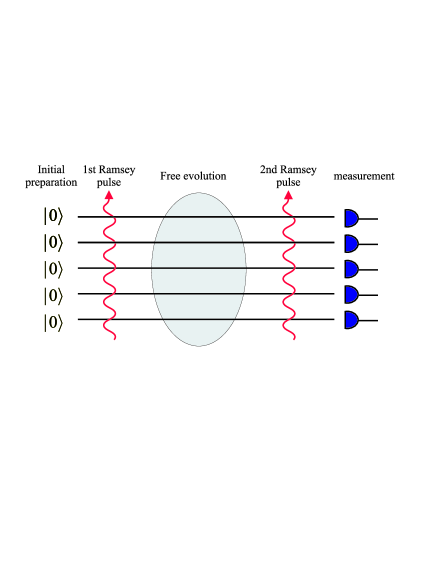
FIG. 1.: Schematic representation of Ramsey spectroscopy with uncorrelated particles.

In the present context standard Ramsey spectroscopy refers to the situation schematically depicted in Fig. 1. An ion trap is loaded with $n$ ions initially prepared in the same internal state $|0\rangle$. A Ramsey pulse of frequency $\omega$ is applied to all ions. The pulse shape and duration are carefully chosen so that it drives the atomic transition $|0\rangle\leftrightarrow|1\rangle$ of natural frequency $\omega_{0}$ and prepares an equally weighted superposition of the two internal states $|0\rangle$ and $|1\rangle$ for each ion. Next the system evolves freely for a time $t$ followed by the second Ramsey pulse. Finally, the internal state of each particle is measured. Provided that the duration of the Ramsey pulses is much smaller than the free evolution time $t$, the probability that an ion is found in $|1\rangle$ is given by

$$P=(1+\cos\Delta\,t)/2.$$ (1)

Here $\Delta=\omega-\omega_{0}$ denotes the detuning between the classical driving field and the atomic transition.

This basic scheme is repeated yielding a total duration $T$ of the experiment. The aim is to estimate $\Delta$ as accurately as possible for a given $T$ and a given number of ions $n$. The two quantities $T$ and $n$ are the physical resources we consider when comparing the performance of different schemes. The statistical fluctuations associated with a finite sample yield an uncertainty $\Delta P$ in the estimated value of $P$ given by

$${\Delta P}=\sqrt{P(1-P)/N}$$ (2)

where $N=nT/t$ denotes the actual number of experimental data (we assume that $N$ is large). Hence the uncertainty in the estimated value of $\omega_{0}$ is given by:

$${|\delta\omega_{0}|}=\frac{\sqrt{P(1-P)/N}}{|dP/d\omega|} ={{1}\over{\sqrt{nTt}}}.$$ (3)

This value is often referred to as the shot noise limit [3].

The theoretical possibility of overcoming this limit has been put forward recently [4, 5]. The basic idea is to prepare the ions initially in an entangled state, which for small $n$ seems to be practical in the near future. To see the advantage of this approach, let us consider the case of two ions prepared in the maximally entangled state [6]

$$|\Psi\rangle=(|00\rangle+|11\rangle)/\sqrt{2}.$$ (4)

This state can be generated, for example, by the initial part of the network illustrated in Fig. 2. A Ramsey pulse on the first ion is followed by a controlled–NOT gate [7]. After a free evolution period of time $t$ the state of the composite system in the interaction picture rotating at the driving frequency $\omega$ reads

$$|\Psi\rangle=(|00\rangle+e^{-2i\Delta t}\,|11\rangle)/\sqrt{2}\;.$$ (5)

The second part of the network allows to disentangle the ions after the free evolution period. The population in state $|1\rangle$ of the first ion will now oscillate at a frequency $2\Delta$

$$P_{2}=(1+\cos 2\Delta t)/2.$$ (6)

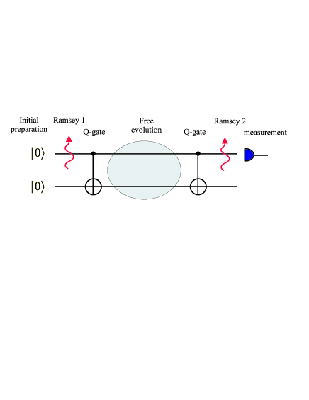
FIG. 2.: Spectroscopy with two maximally entangled particles. The particles are entangled and disentangled by means of “controlled–NOT” gates [7].

This scheme can be easily generalised to the $n$ ion case by a sequence of controlled–NOT gates linking the first ion with each of the remaining ones. In this way, a maximally entangled preparation of $n$ ions of the form

$$|\Psi\rangle=(|00...0\rangle+|11...1\rangle)/\sqrt{2}$$ (7)

is generated. The final measurement on the first ion, after the free evolution period and the second set of controlled–NOT gates, gives the signal

$$P_{n}=(1+\cos n\Delta t)/2\;.$$ (8)

The advantage of this scheme is that the oscillation frequency of the signal is now amplified by a factor $n$ with respect to the case of uncorrelated ions and the corresponding frequency uncertainty is

$${|\delta\omega_{0}|}={{1}\over{n\sqrt{Tt}}}.$$ (9)

Note that this result represents an improvement of a factor $1/\sqrt{n}$ over the shot noise limit (3) by using the same number of ions $n$ and the same total duration of the experiment $T$ [8] and it was argued that this is the best precision possible [9].

Let us now examine the same situation in a realistic experimental scenario, where decoherence effects are inevitably present. The main type of decoherence in an ion trap is dephasing due to processes that cause random phase changes while preserving the population in the atomic levels. Important mechanisms that result in dephasing effects are collisions, stray fields and laser instabilities. We model the time evolution of the reduced density operator for a single ion $\rho$ in the presence of decoherence by the following master equation [10]:

$$\dot{\rho}(t)=i\Delta\left(\rho|1\rangle\langle 1|-|1\rangle\langle 1|\rho\right)+\gamma\left(\sigma_{z}\rho\sigma_{z}-\rho\right)$$ (10)

the density matrix decay [Actually, our analysis is not restricted to this particular model but holds for any process where off-diagonal elements decay exponentially with time.] Equation (10) is written in a frame rotating at the frequency $\omega$. By $\sigma_{z}=|0\rangle\langle 0|-|1\rangle\langle 1|$ we denote a Pauli spin operators. Here we have introduced the decay rate $\gamma=1/\tau_{dec}$, where $\tau_{dec}$ is the decoherence time. For the case of standard Ramsey spectroscopy this will give rise to a broadening of signal (1):

$$P=(1+\cos\Delta\,te^{-\gamma t})/2.$$ (11)

As a consequence the corresponding uncertainty in the atomic frequency is no longer $\Delta$-independent. We now have

$${|\delta\omega_{0}|}=\sqrt{{{1-\cos^{2}(\Delta t)e^{-2\gamma t}}\over{nTte^{-2\gamma t}}\sin^{2}(\Delta t)}}\;.$$ (12)

In order to obtain the best precision it is necessary to optimise this expression as a function of the duration of each single measurement $t$. The minimal value is attained for

$$\begin{array}[]{c}\Delta t=k\pi/2\,\,(k\;\;odd)\\ t=\tau_{dec}/2\end{array}$$ (15)

provided that $T>\tau_{dec}/2$. Thus the minimum frequency uncertainty reads

$${|\delta\omega_{0}|}_{opt}=\sqrt{{{2\gamma e}\over{nT}}}=\sqrt{{{2e}\over{n\tau_{dec}T}}}.$$ (16)

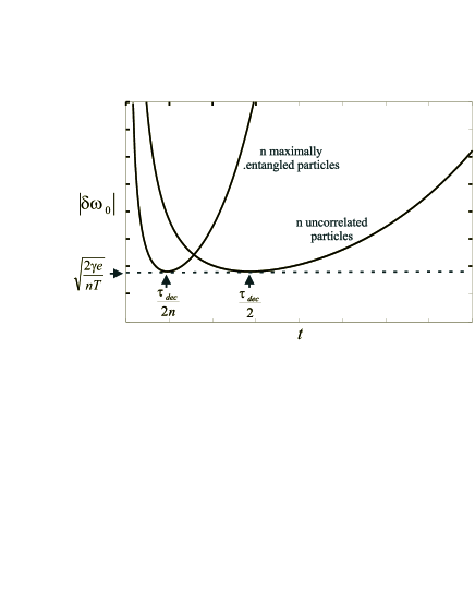
FIG. 3.: Frequency uncertainty $|\delta\omega_{0}|$ as a function of the duration of a single shot $t$ for maximally entangled and uncorrelated particles. Note that the minimum uncertainty is exactly the same for both configurations.

For maximally entangled preparation the signal (8) in the presence of dephasing is modified as follows:

$$P_{n}=(1+\cos n\Delta\,te^{-n\gamma t})/2$$ (17)

and the resulting uncertainty for the estimated value of the atomic frequency is now minimal when

$$\begin{array}[]{c}\Delta t=k\pi/2n\,\,(k\;\;odd)\\ t=\tau_{dec}/2n\end{array}.$$ (20)

Interestingly, we recover exactly the same minimal uncertainty as for standard Ramsey spectroscopy (16). This effect is illustrated in Fig. 3. The modulus of the frequency uncertainty $|\delta\omega_{0}|$ is plotted as a function of the duration of each single experiment $t$ for standard Ramsey spectroscopy with $n$ uncorrelated particles and for a maximally entangled state with $n$ particles. In the presence of decoherence both preparations reach the same precision. This result can be intuitively understood by considering that maximally entangled states are much more fragile in the presence of decoherence: their decoherence time is reduced by a factor $n$ and therefore the duration of each single experiment $t$ has also to be reduced by the same amount. Moreover, the limit (16) represents the best accuracy for both uncorrelated and maximally entangled preparations and cannot be overcome by engineering different kinds of measurements as will be shown below.

Note that the problem addressed in precision spectroscopy (i.e. the measurement of small atomic phase shifts) maps onto that of statistical distinguishability of nearby states, analyzed by Wootters [11] and generalized by Braunstein and Caves [12, 13]. They have provided an upper bound for the precision in the estimation of a given variable that parametrizes a family of quantum states. In our case this variable is the detuning $\Delta$. Moreover, the optimal measurements always correspond to a set of orthogonal projectors in the $n$ ions Hilbert space. It is worthwhile pointing out the generality of this result in the sense that it accounts for any possible joint measurement on the $n$ particles and any method of data analysis. When the Braunstein and Caves optimization procedure is applied to either uncorrelated or maximally entangled preparations of $n$ ions it yields the same limit (16).

However, we will show in the following that with certain partially entangled preparations one can overcome the limit (16). Let us analyze first the case of generalized Ramsey spectroscopy, namely a scheme where the operator

$$S_{x}=\sum_{k=1}^{n}\sigma_{x}^{k}$$ (21)

is measured after the free evolution period. In (21) $\sigma_{x}=|1\rangle\langle 0|+|0\rangle\langle 1|$ denotes the Pauli spin operator and the superscript $k$ refers to the $k$th particle.

We can easily evaluate the expectation values of the operators $S_{x}$ and $S_{x}^{2}$ in terms of the corresponding quantities in the absence of decoherence:

$$\langle S_{x}\rangle\equiv\langle\sum_{k=1}^{n}\sigma_{x}^{k}\rangle=e^{-\gamma t}\langle S_{x}(\gamma=0)\rangle$$ (22)

$$\langle S_{x}^{2}\rangle=n+\langle\sum_{l\neq m}\sigma_{x}^{l}\sigma_{x}^{m}\rangle=n+e^{-2\gamma t}(\langle S_{x}^{2}(\gamma=0)\rangle-n).$$ (23)

Finally, the resulting uncertainty in the atomic frequency is given by

$${|\delta\omega_{o}|}=\sqrt{{1\over N}{{(\Delta S_{x})^{2}}\over{\left({{\partial\langle S_{x}\rangle}\over{\partial\omega}}\right)^{2}}}}$$ (24)

where $\langle\Delta S_{x}\rangle^{2}=\langle S_{x}^{2}\rangle-\langle S_{x}\rangle^{2}$ and $N$ denotes the total number of measurements performed during the total time $T$. A straightforward calculation leads to an optimal duration of each measurement $t_{opt}$ given by the solution of the following equation [14]

$$n[1+(2\gamma t-1)e^{2\gamma t}]=\langle\Delta S_{y}(t=0)\rangle^{2}$$ (25)

and the corresponding sensitivity takes the form

$${|\delta\omega_{o}|_{opt}}=\sqrt{{{2n\gamma e^{2\gamma t_{opt}}}\over{T\langle S_{x}(t=0)\rangle^{2}}}}$$ (26)

where $\langle S_{x}(t=0)\rangle$ and $\langle S_{y}(t=0)\rangle^{2}$ refer to the initial state preparation. The subscript opt emphasizes that optimization with respect to $\Delta t$ has already been taken into account, the minimum value being achieved for $\Delta t=\pi/2$. Notice that each initial preparation is optimized for different values of the single shot time. We can now state a lower bound for the precision attainable within this approach as follows:

$${|\delta\omega_{o}|_{opt}}\geq\sqrt{{{2n\gamma}\over{T\langle S_{x}(0)\rangle^{2}}}}\geq\sqrt{{{2}\over{n\tau_{dec}T}}}.$$ (27)

Compared with the results above, a maximum improvement of $1/\sqrt{e}$ in the resolution can be achieved. Thus we have found that the bound (16) can be overcome for certain partially entangled states [15].

We now analyze the best precision that can be achieved when optimizing the experiment with respect to both the initial state preparation and the final measurement. The problem has been studied by means of a numerical optimization procedure and we have restricted ourselves to small numbers of ions in the trap. The initial state preparation which leads to the best precision is of the form

$$|\psi_{n}\rangle=\sum_{k=0}^{\lfloor\frac{n}{2}\rfloor}a_{k}|k\rangle\;,$$ (28)

where $|k\rangle$ denotes an equally weighted superposition of all states of $n$ ions which contain either a number $k$ or a number $n-k$ of excited states. By $\lfloor\cdots\rfloor$ we denote the corresponding integer part. The coefficients $a_{k}$ can be chosen to be real. For example, the corresponding family of states for $n=4$ reads

$$|\psi_{4}\rangle=a_{0}(|0000\rangle+|1111\rangle)+a_{1}(|0001\rangle+|0010\rangle$$ (29)

$$+|0100\rangle+|1000\rangle+|1110\rangle+|1101\rangle+|1011\rangle+|0111\rangle)$$ (30)

$$+a_{2}(|0011\rangle+|0101\rangle+|1001\rangle+|1100\rangle+|1010\rangle+|0110\rangle)\;.$$ (31)

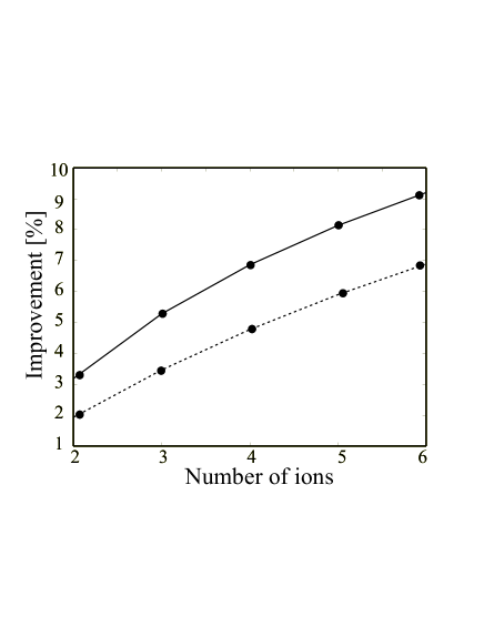
FIG. 4.: The optimum percentual improvement in the precision relative to the limit (16) as a function of the number of ions $n$. Solid line: Numerical optimization with respect to the initial preparation and application of the Braunstein and Caves algorithm for determinig the optimal measurement. Dashed line: Optimized initial preparation and generalized Ramsey spectroscopy as the final measurement.

Note that this family of states exhibits a high degree of symmetry: it is completely symmetric under permutations of the $n$ ions and under exchange of the excited and the ground state for each ion. The optimum percentual improvement in the precision relative to the limit (16) as a function of the number of ions $n$ is shown in Fig. 4. The solid curve shows the improvement obtained by optimizing both the inital preparation and the final measurement using the algorithm of Braunstein and Caves. The dashed line exhibits the improvement obtained by optimizing only the initial preparation and performing the measurement given in Eq. (21) corresponding to generalized Ramsey spectroscopy. The improvement obtained by optimising the measurement is rather small. The question whether the (dashed) curve corresponding to Ramsey spectroscopy asymptotically saturates at the theoretical limit (27) or below remains to be addressed. Moreover, whether the curve corresponding to Braunstein and Caves optimization saturates at the same value or higher than the Ramsey curve is an open question.

In conclusion, we can state that standard Ramsey spectroscopy is optimal for uncorrelated particles both in the presence and in the absence of decoherence effects. The use of maximally entangled states does not provide higher resolution as compared to using independent particles when decoherence is present. The best sensitivity is achieved when the ions are initially prepared in highly symmetric but only partially entangled states.

We are grateful to A. Barenco, L. Cutler, G.M. D’Ariano, R. Derka, C.A. Fuchs, H.J. Kimble, P.L. Knight, H. Mabuchi, A. Steane, S. Williams, D.J. Wineland and P. Zoller for stimulating discussions.

This work was supported in part by the European TMR Research Network ERB 4061PL95-1412, the European TMR Research Network on Cavity QED, the Royal Society, Hewlett-Packard, Elsag-Bailey and the Alexander von Humbold Stiftung. SFH acknowledges support from by DGICYT Project No. PB-95-0594 (Spain). CM is supported by a TMR “Marie Curie” Fellowship. TP holds an “Erwin–Schrödinger” scholarship granted by the Austrian Science Fund. We also acknowledge private support from Otto Pellizzari.

REFERENCES

- [1] Also at: I.S.I. Foundation, Villa Gualino, V.le Settimio Severo 63, 10133 Torino, Italy.
- [2] D. J. Wineland et al., IEEE Trans. on Ultrasonics, Ferroelectrics and Frequency Control A37, 515 (1990)
- [3] W. H. Itano et al., Phys. Rev. A47, 3554 (1993).
- [4] W. J. Wineland et al., Phys. Rev. A46, R6797 (1992).
- [5] D. J. Wineland et al., Phys. Rev. A50, 67 (1994).
-
[6]
We note this particular example does not represent exactly the original
proposal by Wineland
et al. [4, 5]. We have modified it to fit
the presentation in the paper, however, the two schemes are equivalent
as far as the resulting precision is concerned.
- [7] A. Barenco et al., Phys. Rev. Lett. 74, 4083 (1995).
- [8] In reference [4] also certain partially entangled preparations are analyzed which yield an improvement over the shot noise.
- [9] J. J. Bollinger et al., Phys. Rev. A54, R4649 (1996).
- [10] C. W. Gardiner, Quantum Noise (Springer–Verlag, Berlin 1991).
- [11] W. K. Wooters, Phys. Rev. D23,357 (1981)
- [12] S. L. Braunstein and C. Caves, Phys. Rev. Lett. 72, 3439 (1994)
- [13] S. L. Braunstein, C. Caves and G. J. Milburn, Annals of Physics 247, 135 (1996)
- [14] We have restricted ourselves to the same preparations as the ones analyzed in [4] where only states yielding a resonance curve symmetric about are considered.
- [15] For example, for these states are of the form with real coefficients and . For and we have a 2 improvement in the sensitivity with respect to (16).