Generation of single-mode SU(1,1) intelligent states and an analytic approach to their quantum statistical properties

Abstract

We discuss a scheme for generation of single-mode photon states associated with the two-photon realization of the SU(1,1) algebra. This scheme is based on the process of non-degenerate down-conversion with the signal prepared initially in the squeezed vacuum state and with a measurement of the photon number in one of the output modes. We focus on the generation and properties of single-mode SU(1,1) intelligent states which minimize the uncertainty relations for Hermitian generators of the group. Properties of the intelligent states are studied by using a “weak” extension of the analytic representation in the unit disk. Then we are able to obtain exact analytical expressions for expectation values describing quantum statistical properties of the SU(1,1) intelligent states. Attention is mainly devoted to the study of photon statistics and linear and quadratic squeezing.

PACS numbers: 42.50.Dv, 03.65.Fd

1 Introduction

Intelligent states are quantum states which minimize uncertainty relations for non-commuting quantum observables [1–3]. In the last years there exists a great interest in various properties, applications and generalizations of intelligent states [4–22]. One of the reasons for this interest is the close relationship between intelligent states and squeezing. For example, the generalized intelligent states of the Weyl-Heisenberg group coincide with the canonical squeezed states. In fact, the generalized intelligent states for two quantum observables can provide an arbitrarily strong squeezing in either of them [8]. Therefore, a generalization of squeezed states for an arbitrary dynamical symmetry group leads to the intelligent states for the group generators [5, 8]. In particular, the concept of squeezing can be naturally extended to the intelligent states associated with the SU(2) and SU(1,1) Lie groups. An important possible application of squeezing properties of the SU(2) and SU(1,1) intelligent states is the reduction of the quantum noise in spectroscopy [10] and interferometry [6, 15].

In the present paper we propose a scheme for generation of intelligent photon states associated with the two-photon realization of the SU(1,1) algebra. This scheme is based on a combination of degenerate and non-degenerate optical parametric processes, with a measurement of the photon number in one of the output modes. In order to study properties of the intelligent states, we use a “weak” extension of the analytic representation in the unit disk [23]. In the context of the two-photon realization, this analytic representation is based on the single-mode squeezed states. The bases of the squeezed vacuum states and the squeezed “one photon” states are used in the even and odd sectors of the Fock space, respectively. Thus we obtain the analytic representations of various eigenstates associated with the SU(1,1) algebra. Using these representations, we derive exact closed expressions for moments of the SU(1,1) generators. In this way we are able to study various quantum statistical properties of photon states whose generation is possible in the presented scheme. We devote attention to the examination of photon statistics and linear and quadratic squeezing. We show that the single-mode SU(1,1) intelligent states exhibit interesting nonclassical properties such as sub-Poissonian photon statistics and strong squeezing.

2 The SU(1,1) intelligent states

In this work we consider two-photon parametric processes. Hamiltonians describing these processes involve operators of the form $a^{2}$ and $a^{\dagger 2}$, where $a$ is the annihilation operator of a quantized light mode. It is convenient to use the operators

$$K_{+}=\mbox{$\frac{1}{2}$}a^{\dagger 2}\hskip 22.76228ptK_{-}=\mbox{$\frac{1}{2}$}a^{2}\hskip 22.76228ptK_{3}=\mbox{$\frac{1}{2}$}a^{\dagger}a+\mbox{$\frac{1}{4}$}$$ (2.1)

which form the single-mode two-photon realization of the SU(1,1) Lie algebra,

$$[K_{-},K_{+}]=2K_{3}\hskip 22.76228pt[K_{3},K_{\pm}]=\pm K_{\pm}\,.$$ (2.2)

One can also use the Hermitian combinations $K_{1}=\frac{1}{2}(K_{+}+K_{-})$ and $K_{2}=\frac{1}{2{\rm i}}(K_{+}-K_{-})$ which satisfy the well-known SU(1,1) commutation relations. The Casimir operator $K^{2}$ for any irreducible representation is the identity operator multiplied by a number,

$$K^{2}=K_{3}^{2}-K_{1}^{2}-K_{2}^{2}=k(k-1)I\,.$$ (2.3)

Thus a representation of SU(1,1) is determined by the number $k$ called the Bargmann index [24]. The representation space ${\cal H}_{k}$ is spanned by the orthonormal basis $|n,k\rangle$ ($n=0,1,2,\ldots$). For the two-photon realization (2.1), one obtains $K^{2}=-3/16$. Therefore, there are two irreducible representations: $k=1/4$ and $k=3/4$ [25]. The representation space ${\cal H}_{e}$ ($k=1/4$) is the even Fock subspace with the orthonormal basis consisting of even number states $|n,\frac{1}{4}\rangle=|2n\rangle$ ($n=0,1,2,\ldots$); the representation space ${\cal H}_{o}$ ($k=3/4$) is the odd Fock subspace with the orthonormal basis consisting of odd number states $|n,\frac{3}{4}\rangle=|2n+1\rangle$ ($n=0,1,2,\ldots$).

Any two quantum observables (Hermitian operators in the Hilbert space) $A$ and $B$ obey the generalized uncertainty relation

$$(\Delta A)^{2}(\Delta B)^{2}\geq\frac{1}{4}\left(\langle C\rangle^{2}+4\Delta_{AB}^{2}\right)\hskip 22.76228ptC=-{\rm i}[A,B]$$ (2.4)

where the variance of $A$ is $(\Delta A)^{2}=\langle A^{2}\rangle-\langle A\rangle^{2}$, $(\Delta B)^{2}$ is defined similarly, the covariance of $A$ and $B$ is $\Delta_{AB}=\frac{1}{2}\langle AB+BA\rangle-\langle A\rangle\langle B\rangle$, and the expectation values are taken over an arbitrary state in the Hilbert space. When the covariance of $A$ and $B$ vanishes, $\Delta_{AB}=0$, the generalized uncertainty relation (2.4) reduces to the ordinary uncertainty relation

$$(\Delta A)^{2}(\Delta B)^{2}\geq\frac{1}{4}\langle C\rangle^{2}\,.$$ (2.5)

Ordinary and generalized intelligent states provide an equality in the ordinary and generalized uncertainty relations (2.5) and (2.4), respectively [8]. The intelligent states for operators $A$ and $B$ are determined by the eigenvalue equation [8, 9]

$$(\eta A+{\rm i}B)|\psi\rangle=\lambda|\psi\rangle\$$ (2.6)

where $\lambda$ is a complex eigenvalue. The parameter $\eta$ is complex for the generalized intelligent states and real for the ordinary ones. For ${\rm Re}\,\eta\neq 0$, expectation values over the intelligent states satisfy [8]:

$$\langle A\rangle=\frac{{\rm Re}\,\lambda}{{\rm Re}\,\eta}\hskip 22.76228pt\langle B\rangle={\rm Im}\,\lambda-\frac{{\rm Im}\,\eta}{{\rm Re}\,\eta}\,{\rm Re}\,\lambda$$ (2.7)

$$(\Delta A)^{2}=\frac{\langle C\rangle}{2{\rm Re}\,\eta}\hskip 22.76228pt(\Delta B)^{2}=\frac{|\eta|^{2}\langle C\rangle}{2{\rm Re}\,\eta}\hskip 22.76228pt\Delta_{AB}=-\frac{{\rm Im}\,\eta}{2{\rm Re}\,\eta}\langle C\rangle\,.$$ (2.8)

In the present work we consider the generation of the single-mode SU(1,1) intelligent states. According to the above definitions, the eigenvalue equation $(\eta K_{2}+{\rm i}K_{3})|\psi\rangle=\lambda|\psi\rangle$ with real $\eta$ determines the ordinary intelligent states for the SU(1,1) generators $K_{2}$ and $K_{3}$. It means that these states provide an equality in the uncertainty relation $(\Delta K_{2})^{2}(\Delta K_{3})^{2}\geq\mbox{$\frac{1}{4}$}\langle K_{1}\rangle^{2}$. Analogously, the eigenvalue equation $(\eta K_{1}-{\rm i}K_{2})|\psi\rangle=\lambda|\psi\rangle$ with real $\eta$ determines the ordinary intelligent states for the SU(1,1) generators $K_{1}$ and $K_{2}$. These states provide an equality in the uncertainty relation $(\Delta K_{1})^{2}(\Delta K_{2})^{2}\geq\mbox{$\frac{1}{4}$}\langle K_{3}\rangle^{2}$.

3 The generation scheme

Some schemes for the experimental production of the SU(2) and SU(1,1) intelligent states in nonlinear optical processes have been suggested recently [13, 14, 17]. We focus on the most recent scheme, developed by Luis and Peřina [17], which employs two important quantum mechanical features. The first one is the entangled nature of the two-mode field generated by parametric down-conversion, and the second one is the role of measurement as a way to manipulate the state of an entangled quantum system.

It is known that in non-degenerate parametric down-conversion a measurement in the idler mode can be used to affect the state of the signal mode [26–31]. In particular, near-number states can be obtained in the signal mode by the measurement of the photon number in the idler mode [26]. Luis and Peřina [17] consider in their scheme two parametric down-conversion crystals with aligned idler beams and show that the measurement of the photon number in some of the modes leads to states which are related to the two-mode SU(2) and SU(1,1) coherent and intelligent states. The basic idea of this method is related to an interference experiment with signal beams coming from two parametric down-conversion crystals with aligned idler beams [32, 33].

In the present paper we consider a modification of the Luis-Peřina scheme, which is suitable for the generation of the single-mode SU(1,1) intelligent states. To this end, we examine the states produced in parametric down-conversion with the signal mode prepared in the squeezed vacuum state, after the measurement of the photon number in one of the output modes. We show that this simple scheme produces the eigenstates of a linear combination of the two-photon SU(1,1) generators. An additional SU(1,1) transformation, implemented by a degenerate parametric amplifier, takes these states into the single-mode SU(1,1) intelligent states.

The scheme under discussion is outlined in figure 1. Two light beams represented by the mode annihilation operators $a$ and $b$ are mixed in the non-degenerate parametric amplifier NPA. The mode $a$ is beforehand squeezed in the degenerate parametric amplifier DPA. We assume that both parametric amplifiers are coherently pumped by strong and undepleted classical fields, and that the system is free of losses.

Figure 1: Outline of the generation scheme. The light mode $a$ is squeezed in the degenerate parametric amplifier DPA. Then the two light modes $a$ and $b$ are mixed in the non-degenerate parametric amplifier NPA.

The processes of degenerate and non-degenerate parametric amplification are described by effective interaction Hamiltonians $H_{1}$ and $H_{2}$, respectively,

$$H_{1}=\mbox{$\frac{1}{2}$}g_{1}a^{\dagger 2}+\mbox{$\frac{1}{2}$}g_{1}^{\ast}a^{2}\hskip 22.76228ptH_{2}=g_{2}a^{\dagger}b^{\dagger}+g_{2}^{\ast}ab$$ (3.1)

where $\hbar=1$ and $g_{1}$, $g_{2}$ are parameters depending on the pump and the nonlinear characteristics of the media. The output state $|\psi\rangle$ of the whole system is related to the input state $|\psi\rangle_{\rm in}$ by the unitary transformation $U$,

$$|\psi\rangle=U|\psi\rangle_{\rm in}\hskip 22.76228ptU=U_{2}U_{1}=\exp(-{\rm i}H_{2}t_{2})\exp(-{\rm i}H_{1}t_{1})$$ (3.2)

where $t_{1}$, $t_{2}$ are the interaction times. We consider the input field in the vacuum state, $|\psi\rangle_{\rm in}=|0\rangle_{a}|0\rangle_{b}$. The mode $a$ is squeezed in DPA, and it enters NPA in the squeezed vacuum state. There is no need to take into account explicitly the free propagation of the mode $a$ between DPA and NPA, since this only changes the phase angle of squeezing.

The input state $|\psi\rangle_{\rm in}$ satisfies the vacuum condition, $a|\psi\rangle_{\rm in}=b|\psi\rangle_{\rm in}=0$, i.e. it is an eigenstate of the annihilation operators. Using this property, we find that the output state satisfies the equations

$$UaU^{\dagger}|\psi\rangle=(\mu_{1}\mu_{2}a+\nu_{1}\nu_{2}^{\ast}b-\nu_{1}\mu_{2}a^{\dagger}-\mu_{1}\nu_{2}b^{\dagger})|\psi\rangle=0$$ (3.3)

$$UbU^{\dagger}|\psi\rangle=(\mu_{2}b-\nu_{2}a^{\dagger})|\psi\rangle=0$$ (3.4)

where we have introduced the following notation

$$\xi_{j}=-{\rm i}g_{j}t_{j}=|\xi_{j}|\,e^{{\rm i}\theta_{j}}\hskip 22.76228pt\mu_{j}=\cosh|\xi_{j}|\hskip 22.76228pt\nu_{j}=\sinh|\xi_{j}|\,e^{{\rm i}\theta_{j}}\hskip 22.76228ptj=1,2.$$ (3.5)

We next assume that a measurement of the number of photons is performed in one of the output beams by an ideal photodetector with perfect quantum efficiency. The outcome of the measurement is denoted by $n$. The state in the remaining mode after this measurement is given by the projection of the number state $|n\rangle_{i}$ on $|\psi\rangle$,

$$|\psi_{n}\rangle={}_{i}\langle n|\psi\rangle$$ (3.6)

where $i$ is either $a$ or $b$, depending in which mode the measurement has been performed.

We first consider the case of the photon-number measurement in the mode $b$. The reduced eigenvalue equation for the state $|\psi_{n}\rangle$ can be obtained from equations (3.3) and (3.4) by rewriting them in the form

$$b^{\dagger}b|\psi\rangle=(a^{\dagger}a-\chi a^{\dagger 2})|\psi\rangle$$ (3.7)

where we have defined

$$\chi=\frac{\nu_{1}}{\mu_{1}\mu_{2}^{2}}=\frac{\tanh|\xi_{1}|}{\cosh^{2}|\xi_{2}|}\,e^{{\rm i}\theta_{1}}\,.$$ (3.8)

Note that $|\chi|<1$. The eigenvalue equation for $|\psi_{n}\rangle$ is obtained now by projecting (3.7) over the number state $|n\rangle_{b}$. This gives

$$(a^{\dagger}a-\chi a^{\dagger 2})|\psi_{n}\rangle=n|\psi_{n}\rangle\,.$$ (3.9)

In terms of the SU(1,1) generators, equation (3.9) can be written as

$$(K_{3}-\chi K_{+})|\psi_{n}\rangle=(k+l)|\psi_{n}\rangle$$ (3.10)

where $l$ is a non-negative integer defined by

$$l=\left[\frac{n}{2}\right]=\left\{\begin{array}[]{l}n/2\hskip 11.38092pt\mbox{for $n$ even}\;(k=1/4)\\ (n-1)/2\hskip 11.38092pt\mbox{for $n$ odd}\;(k=3/4)\,.\end{array}\right.$$ (3.11)

According to this definition, $n=2l+2k-\frac{1}{2}$. We see that the state $|\psi_{n}\rangle$ belongs to the even representation ($k=1/4$) for even $n$, and to the odd representation ($k=3/4$) for odd $n$. We also see that in the limit $\chi\rightarrow 0$ (i.e. $\xi_{1}\rightarrow 0$) the state $|\psi_{n}\rangle$ approaches the number state $|n\rangle$ (an eigenstate of $K_{3}$). This behavior is easily understood by recalling that for $\xi_{1}=0$ the mode $a$ enters NPA in the vacuum state. Thus we recover the particular case in which the number states are generated.

Let us now consider the effect of performing an additional transformation on the mode $a$. We assume that this mode, after it has been prepared in the state $|\psi_{n}\rangle$, accumulates a phase shift $\varphi$ and is then once again squeezed in a lossless degenerate parametric amplifier with a classical coherent pump. Both these processes can be represented as SU(1,1) transformations, and the final state $|\bar{\psi}_{n}\rangle$ is given by

$$|\bar{\psi}_{n}\rangle=\exp(-{\rm i}\omega K_{2})\exp(-{\rm i}\varphi K_{3})|\psi_{n}\rangle\,.$$ (3.12)

If we choose

$$\varphi={\rm arg}\,\chi=\theta_{1}\hskip 22.76228pt\tanh\omega=|\chi|,$$ (3.13)

the final state $|\bar{\psi}_{n}\rangle$ will satisfy the eigenvalue equation

$$(\eta K_{2}+{\rm i}K_{3})|\bar{\psi}_{n}\rangle={\rm i}(k+l)\sqrt{\eta^{2}+1}\,|\bar{\psi}_{n}\rangle\,.$$ (3.14)

The real parameter $\eta$ is defined as

$$\eta=\sinh\omega=\frac{|\chi|}{\sqrt{1-|\chi|^{2}}}\,.$$ (3.15)

The states $|\bar{\psi}_{n}\rangle$ of equation (3.14) are easily recognized as the $K_{2}$-$K_{3}$ intelligent states.

We next consider the case of the photon-number measurement in the mode $a$. It turns out that this situation contains more possibilities than the previous one. The reduced eigenvalue equation for the state $|\psi_{n}\rangle$ is obtained from equations (3.3) and (3.4) by rewriting them in the form

$$a^{\dagger}a|\psi\rangle=(b^{\dagger}b+\chi b^{2})|\psi\rangle$$ (3.16)

where we have defined

$$\chi=\frac{\nu_{1}}{\mu_{1}\nu_{2}^{2}}=\frac{\tanh|\xi_{1}|}{\sinh^{2}|\xi_{2}|}\,e^{{\rm i}(\theta_{1}-2\theta_{2})}\,.$$ (3.17)

Note that here $0<|\chi|<\infty$. The eigenvalue equation for $|\psi_{n}\rangle$ is obtained now by projecting (3.16) over the number state $|n\rangle_{a}$. This gives

$$(b^{\dagger}b+\chi b^{2})|\psi_{n}\rangle=n|\psi_{n}\rangle\,.$$ (3.18)

In terms of the SU(1,1) generators, this equation takes the form

$$(K_{3}+\chi K_{-})|\psi_{n}\rangle=(k+l)|\psi_{n}\rangle$$ (3.19)

where $l$ is a non-negative integer defined by equation (3.11). Once again, the state $|\psi_{n}\rangle$ belongs to the even representation ($k=1/4$) for even $n$, and to the odd representation ($k=3/4$) for odd $n$. For $\chi\rightarrow 0$ (i.e. $\xi_{1}\rightarrow 0$), we again go back to the situation where both modes entering NPA are in the vacuum state, and the photon-number measurement in one of the output modes leads to the number state in the other.

Also, we consider the effect of additional SU(1,1) transformations performed on the mode $b$, after it has been prepared in the state $|\psi_{n}\rangle$. The final state $|\bar{\psi}_{n}\rangle$ is given by

$$|\bar{\psi}_{n}\rangle=\exp({\rm i}\omega K_{2})\exp({\rm i}\varphi K_{3})|\psi_{n}\rangle\,.$$ (3.20)

It is convenient to choose

$$\varphi={\rm arg}\,\chi=\theta_{1}-2\theta_{2}\,.$$ (3.21)

It is necessary to distinguish here between the two possibilities: $|\chi|<1$ and $|\chi|>1$. When $|\chi|<1$, we choose

$$\tanh\omega=|\chi|,$$ (3.22)

which leads to the eigenvalue equation (3.14) with the real parameter $\eta$ given by (3.15) but with $\chi$ of equation (3.17). In this case we once again obtain the $K_{2}$-$K_{3}$ intelligent states.

The case $|\chi|>1$ is different. Here we choose

$$\coth\omega=|\chi|,$$ (3.23)

which leads to the eigenvalue equation

$$(\eta K_{1}-{\rm i}K_{2})|\bar{\psi}_{n}\rangle=(k+l)\sqrt{1-\eta^{2}}\,|\bar{\psi}_{n}\rangle\,.$$ (3.24)

The real parameter $\eta$ is defined as

$$\eta=\frac{1}{\cosh\omega}=\frac{\sqrt{|\chi|^{2}-1}}{|\chi|}\,.$$ (3.25)

Note that here $0<\eta<1$. The states $|\bar{\psi}_{n}\rangle$ of equation (3.24) are recognized as the $K_{1}$-$K_{2}$ intelligent states.

4 Analytic representations

In this section we present an analytic formalism that provides a complete solution to the eigenvalue problem involving any linear combination of the SU(1,1) generators [19]. In partcular, we are able to solve the eigenvalue equations that define the SU(1,1) intelligent states. For the two-photon realization of SU(1,1), we use a special treatment involving a “weak” resolution of the identity in terms of the squeezed states [23].

4.1 The analytic representation in the unit disk and its “weak” extension

As was discussed by Perelomov [34], each SU(1,1) coherent state corresponds to a point in the coset space SU(1,1)/U(1) that is the upper sheet of the two-sheet hyperboloid (Lobachevski plane). Thus a coherent state is specified by a pseudo-Euclidean unit vector of the form $(\sinh\tau\cos\varphi,\sinh\tau\sin\varphi,\cosh\tau)$. The coherent states $|\zeta,k\rangle$ are obtained by applying unitary operators $\Omega(\xi)\in$ SU(1,1)/U(1) to the lowest state $|n=0,k\rangle$,

$$|\zeta,k\rangle = \exp\left(\xi K_{+}-\,\xi^{\ast}K_{-}\right)|0,k\rangle=(1-|\zeta|^{2})^{k}\exp\left(\zeta K_{+}\right)|0,k\rangle$$ (4.1)

$$= (1-|\zeta|^{2})^{k}\sum_{n=0}^{\infty}\left[\frac{\Gamma(n+2k)}{n!\Gamma(2k)}\right]^{1/2}\!\zeta^{n}|n,k\rangle\,.$$

Here $\xi=-(\tau/2)\,{\rm e}^{-{\rm i}\varphi}$ and $\zeta=(\xi/|\xi|)\tanh|\xi|=-\tanh(\tau/2)\,{\rm e}^{-{\rm i}\varphi}$, so $|\zeta|<1$. The condition $|\zeta|<1$ shows that the SU(1,1) coherent states are defined in the interior of the unit disk. An important property is the resolution of the identity: for $k>1/2$ one gets

$$\int{\rm d}\mu(\zeta,k)|\zeta,k\rangle\langle\zeta,k|=I\mbox{\hskip 42.67912pt}{\rm d}\mu(\zeta,k)=\frac{2k-1}{\pi}\frac{d^{2}\zeta}{(1-|\zeta|^{2})^{2}}$$ (4.2)

where the integration is over the unit disk $|\zeta|<1$. For $k=\frac{1}{2}$ the limit $k\rightarrow\frac{1}{2}$ must be taken after the integration is carried out in the general form. One can represent the state space ${\cal H}_{k}$ as the Hilbert space of analytic functions $G(\zeta;k)$ in the unit disk ${\cal D}(|\zeta|<1)$. They form the so-called Hardy space ${\cal H}({\cal D})$. For a normalized state $|\psi\rangle=\sum_{n=0}^{\infty}C_{n}|n,k\rangle$, one gets

$$G(\zeta;k)=(1-|\zeta|^{2})^{-k}\langle\zeta^{\ast},k|\psi\rangle=\sum_{n=0}^{\infty}C_{n}\left[\frac{\Gamma(n+2k)}{n!\Gamma(2k)}\right]^{1/2}\!\zeta^{n}$$ (4.3)

$$|\psi\rangle=\int{\rm d}\mu(\zeta,k)(1-|\zeta|^{2})^{k}G(\zeta^{\ast};k)|\zeta,k\rangle$$ (4.4)

and the scalar product is

$$\langle\psi_{1}|\psi_{2}\rangle=\int{\rm d}\mu(\zeta,k)(1-|\zeta|^{2})^{2k}[G_{1}(\zeta;k)]^{\ast}G_{2}(\zeta;k)\,.$$ (4.5)

This is the analytic representation in the unit disk.

A serious problem arises for $k<1/2$, when the resolution of the identity (4.2) does not hold. However, another resolution of the identity can be constructed, which is valid for both $k>1/2$ and $k<1/2$ [23]. We point out that in equation (4.3) many functions converge in a disk that is larger than the unit disk. We call ${\cal H}({\cal D}(1+\epsilon))$ the subspace of the Hardy space that contains all the functions that converge in the disk ${\cal D}(1+\epsilon)=\{|\zeta|<1+\epsilon\}$ (where $\epsilon>0$). Clearly if $\epsilon_{1}>\epsilon_{2}$ then ${\cal H}({\cal D}(1+\epsilon_{1}))$ is a subspace of ${\cal H}({\cal D}(1+\epsilon_{2}))$. As $\epsilon$ goes to 0 (from above), ${\cal H}({\cal D}(1+\epsilon))$ becomes the Hardy space. It can be shown [23] that for any positive $k$ apart from integers and half-integers and for any two states in $H({\cal D}(1+\epsilon))$ (where $\epsilon$ is any positive number), the scalar product can be written in the form

$$\langle\psi_{1}|\psi_{2}\rangle=\frac{-(2k-1)\exp(2\pi{\rm i}k)}{4\pi{\rm i}\sin(2\pi k)}\,\oint_{{\cal C}}\frac{{\rm d}t}{(1-t)^{2-2k}}\int_{0}^{2\pi}d\phi\,[G_{1}(\zeta;k)]^{\ast}G_{2}(\zeta;k)$$ (4.6)

where $\zeta=\sqrt{t}\exp({\rm i}\phi)$. The contour ${\cal C}$ is a single loop that goes from the origin up to one below the real axis, turns back around the point $t=1$ in the counter-clockwise direction, and goes back above the real axis up to zero. This contour goes around 1 but is entirely within ${\cal D}(1+\epsilon)$. Equation (4.6) gives a “weak” resolution of the identity which we express as

$$I=\frac{-(2k-1)\exp(2\pi{\rm i}k)}{4\pi{\rm i}\sin(2\pi k)}\oint_{{\cal C}}\frac{{\rm d}t}{(1-t)^{2}}\int_{0}^{2\pi}{\rm d}\phi\,|\zeta,k\rangle\langle\zeta,k|\,.$$ (4.7)

Although the contour ${\cal C}$ goes outside the unit disk, where the SU(1,1) coherent states are not normalisable, this equation has to be understood in a weak sense in conjuction with equation (4.6). The analytic functions $G(\zeta;k)\in H({\cal D}(1+\epsilon))$ are defined according to (4.3), but now

$$|\psi\rangle=\frac{-(2k-1)\exp(2\pi{\rm i}k)}{4\pi{\rm i}\sin(2\pi k)}\oint_{{\cal C}}\frac{{\rm d}t}{(1-t)^{2-k}}\int_{0}^{2\pi}{\rm d}\phi\,G(\zeta^{\ast};k)|\zeta,k\rangle$$ (4.8)

and the scalar product is given by (4.6). Therefore, equations (4.3), (4.6) and (4.8) define the analytic representation in ${\cal D}(1+\epsilon)$.

We can use these results in the context of the two-photon realization, where $k=1/4$ and $k=3/4$. The unitary group operator $\Omega(\xi)\in$ SU(1,1)/U(1) for the two-photon realization is the well-known squeezing operator $S(\xi)$ [35, 36]:

$$S(\xi)=\exp\left(\xi K_{+}-\xi^{\ast}K_{-}\right)=\exp\left(\frac{\xi}{2}a^{\dagger 2}-\frac{\xi^{\ast}}{2}a^{2}\right)\,.$$ (4.9)

Therefore, the SU(1,1) coherent states are the squeezed states. For $k=1/4$ one gets the squeezed vacuum,

$$|\zeta,\mbox{$\frac{1}{4}$}\rangle=S(\xi)|0\rangle=(1-|\zeta|^{2})^{1/4}\sum_{n=0}^{\infty}\frac{\sqrt{(2n)!}}{2^{n}n!}\zeta^{n}|2n\rangle$$ (4.10)

while for $k=3/4$ one gets the squeezed “one photon” state,

$$|\zeta,\mbox{$\frac{3}{4}$}\rangle=S(\xi)|1\rangle=(1-|\zeta|^{2})^{3/4}\sum_{n=0}^{\infty}\frac{\sqrt{(2n+1)!}}{2^{n}n!}\zeta^{n}|2n+1\rangle\,.$$ (4.11)

As before, $\zeta=(\xi/|\xi|)\tanh|\xi|$. It is also possible to define the parity-dependent squeezing operator [37] that imposes different squeezing transformations on the even and odd subspaces of the Fock space. Using the squeezed states, we obtain the following resolutions of the identity (in a weak sense, as explained above):

$$\frac{1}{8\pi}\oint_{{\cal C}}\frac{{\rm d}t}{(1-t)^{2}}\int_{0}^{2\pi}{\rm d}\phi\,|\zeta,\mbox{$\frac{1}{4}$}\rangle\langle\zeta,\mbox{$\frac{1}{4}$}|=I_{e}=\sum_{n=0}^{\infty}|2n\rangle\langle 2n|$$ (4.12)

$$-\frac{1}{8\pi}\oint_{{\cal C}}\frac{{\rm d}t}{(1-t)^{2}}\int_{0}^{2\pi}{\rm d}\phi\,|\zeta,\mbox{$\frac{3}{4}$}\rangle\langle\zeta,\mbox{$\frac{3}{4}$}|=I_{o}=\sum_{n=0}^{\infty}|2n+1\rangle\langle 2n+1|\,.$$ (4.13)

The corresponding analytic representation is given by equations (4.3), (4.6) and (4.8) with $k=1/4$ and $k=3/4$ for states in the even and odd subspaces, respectively. This analytic representation is related to the well-known Bargmann representation through a Laplace transform (see [23] for more details).

4.2 The general eigenvalue problem

Let us consider a linear combination of the SU(1,1) generators of the form

$$(\vec{\beta}\cdot\vec{K})=\beta_{1}K_{1}+\beta_{2}K_{2}+\beta_{3}K_{3}$$ (4.14)

where $\beta_{1}$, $\beta_{2}$ and $\beta_{3}$ are complex parameters. Thus, the operator $(\vec{\beta}\cdot\vec{K})$ belongs to the complexified SU(1,1) algebra. The general eigenvalue problem for the SU(1,1) group can be expressed as [19, 20]:

$$(\vec{\beta}\cdot\vec{K})|\psi\rangle=(\beta_{1}K_{1}+\beta_{2}K_{2}+\beta_{3}K_{3})|\psi\rangle=\lambda|\psi\rangle\hskip 22.76228pt|\psi\rangle\in{\cal H}_{k}\,.$$ (4.15)

Normalized states $|\psi\rangle$ that satisfy this equation are called the SU(1,1) algebra eigenstates [19] or the SU(1,1) algebraic coherent states [20]. Many particular cases of equation (4.15) have been considered in literature. However, the complete solution of the general eigenvalue problem (4.15) has been derived only recently [19], using the analytic representation in the unit disk. We recapitulate here some basic results that are relevant to the single-mode SU(1,1) intelligent states, whose generation we have discussed in section 3. According to equation (4.3), the state $|\psi\rangle$ is represented by the analytic function $G(\zeta;k)$. The SU(1,1) generators act in the Hilbert space of analytic functions $G(\zeta;k)$ as first-order differential operators:

$$K_{+}=\zeta^{2}\frac{d}{d\zeta}+2k\zeta\hskip 22.76228ptK_{-}=\frac{d}{d\zeta}\hskip 22.76228ptK_{3}=\zeta\frac{d}{d\zeta}+k\,.$$ (4.16)

Therefore, the eigenvalue equation (4.15) is transformed into the first-order linear homogeneous differential equation:

$$(\beta_{+}+\beta_{3}\zeta+\beta_{-}\zeta^{2})\frac{d}{d\zeta}G(\zeta;k)+(2k\beta_{-}\zeta+k\beta_{3}-\lambda)G(\zeta;k)=0$$ (4.17)

where we have defined $\beta_{\pm}=(\beta_{1}\pm{\rm i}\beta_{2})/2$. Let us also define

$$B=\sqrt{\beta_{3}^{2}-\beta_{1}^{2}-\beta_{2}^{2}}\,.$$ (4.18)

Note that $B^{2}=(X,X)$ where $X=(\vec{\beta}\cdot\vec{K})$ and $(,)$ is the Killing form [38]. All the operators, whose eigenstates can be produced in the scheme of section 3, are semi-simple elements of the complexified algebra, i.e. their Killing form is non-zero.

For $B\neq 0$ and $\beta_{+}\neq 0$, the solution of equation (4.17) is

$$G(\zeta;k)={\cal N}^{-1/2}(1+\tau_{-}\zeta)^{-k+r}(1+\tau_{+}\zeta)^{-k-r}$$ (4.19)

where ${\cal N}$ is a normalization factor, and we use the following notation:

$$\tau_{\pm}=(\beta_{1}-{\rm i}\beta_{2})/(\beta_{3}\pm B)$$ (4.20)

$$r=\lambda/B\,.$$ (4.21)

Admissible values of $\vec{\beta}$ and $\lambda$ are determined by the requirement that the function $G(\zeta;k)$ must be analytic in the unit disk ${\cal D}$ or, for the “weak” case, in the larger disk ${\cal D}(1+\epsilon)$. If $|\tau_{+}|<(1+\epsilon)^{-1}$ and $|\tau_{-}|<(1+\epsilon)^{-1}$, then there are no restrictions on $\lambda$ (i.e. the corresponding elements of the complexified algebra have a continuous complex spectrum). If $|\tau_{+}|<(1+\epsilon)^{-1}$ and $|\tau_{-}|\geq(1+\epsilon)^{-1}$, then the analyticity condition requires $r=k+l$ (where $l=0,1,2,\ldots$), i.e. the spectrum is discrete and equidistant:

$$\lambda=(k+l)B\,.$$ (4.22)

If $|\tau_{+}|\geq(1+\epsilon)^{-1}$ and $|\tau_{-}|<(1+\epsilon)^{-1}$, then the analyticity condition requires $r=-(k+l)$, and once again the spectrum is discrete and equidistant:

$$\lambda=-(k+l)B\,.$$ (4.23)

If $|\tau_{+}|\geq(1+\epsilon)^{-1}$ and $|\tau_{-}|\geq(1+\epsilon)^{-1}$, then the function $G(\zeta;k)$ of equation (4.19) cannot be analytic in the disk ${\cal D}(1+\epsilon)$ for any value of $\lambda$. This region in the parameter space is forbidden, i.e. the corresponding elements of the complexified algebra have no normalizable eigenstates. According to equations (3.14) and (3.24), the SU(1,1) intelligent states generated in our scheme belong to a class of the algebra eigenstates with the discrete spectrum. For $B\neq 0$ and $\beta_{+}=0$, the solution is

$$G(\zeta;k)={\cal N}^{-1/2}\zeta^{l}(1+\tau_{+}\zeta)^{-2k-l}$$ (4.24)

where $\tau_{+}=\beta_{1}/\beta_{3}$ and $l=-k+\lambda/\beta_{3}$. The condition of the analyticity requires $l=0,1,2,\ldots$ (i.e. the spectrum $\lambda=(k+l)\beta_{3}$ is discrete) and $|\tau_{+}|<(1+\epsilon)^{-1}$. The case of the vanishing Killing form $B=0$ (the so-called degenerate case) has been also discussed in [19].

5 Quantum statistical properties

5.1 Photon statistics and squeezing

Let us consider a normalized state $|\psi\rangle=\sum_{n=0}^{\infty}C_{n}|n,k\rangle$ that belongs to the Hilbert space ${\cal H}_{k}$ of a unitary irreducible representation of SU(1,1). For the two-photon realization of SU(1,1), $|\psi\rangle$ belongs to the even Fock subspace ${\cal H}_{e}$ when $k=1/4$, and to the odd Fock subspace ${\cal H}_{o}$ when $k=3/4$. The photon-number distribution is $P(m)=|\langle m|\psi\rangle|^{2}$, where $|m\rangle$ is a Fock state (photon-number eigenstate). For $k=1/4$, $P(m)$ does not vanish for even $m$ only: $P(2n)=|C_{n}|^{2}$; for $k=3/4$, $P(m)$ does not vanish for odd $m$ only: $P(2n+1)=|C_{n}|^{2}$. The photon-number operator $N=a^{\dagger}a$ can be written as $N=2K_{3}-\frac{1}{2}$. Therefore, the mean photon number and the variance are given by

$$\langle N\rangle=2\langle K_{3}\rangle-\mbox{$\frac{1}{2}$}\hskip 22.76228pt(\Delta N)^{2}=4(\Delta K_{3})^{2}\,.$$ (5.1)

Photon statistics can be conveniently characterized by the intensity correlation function:

$$g^{(2)}=1+\frac{(\Delta N)^{2}-\langle N\rangle}{\langle N\rangle^{2}}\,.$$ (5.2)

Photon statistics is sub- or super-Poissonian for $g^{(2)}<1$ or $g^{(2)}>1$, respectively. The minimal available value of $g^{(2)}$ is zero, corresponding to the maximal possible photon antibunching.

If $A$ and $B$ are two non-commuting observables, $[A,B]={\rm i}C$, the product $(\Delta A)^{2}(\Delta B)^{2}$ taken over a quantum state $|\psi\rangle$ must satisfy the uncertainty relation (2.4). One of the most intriguing phenomena in quantum optics is squeezing, when the quantum noise in one observable is reduced on account of its counter-partner. The state $|\psi\rangle$ is called squeezed in $A$ or $B$, if

$$(\Delta A)^{2}<\mbox{$\frac{1}{2}$}|\langle C\rangle|\;\;\;{\rm or}\;\;\;(\Delta B)^{2}<\mbox{$\frac{1}{2}$}|\langle C\rangle|\,.$$ (5.3)

It is clear that the ordinary intelligent state, for which $(\Delta A)^{2}(\Delta B)^{2}=\frac{1}{4}\langle C\rangle^{2}$, is squeezed in either $A$ or $B$ whenever the two uncertainties are unequal. Note that condition (5.3) determines a relation between uncertainties of $A$ and $B$. However, the uncertainty of the squeezed observable can be quite large if $\frac{1}{2}|\langle C\rangle|$ is large. Therefore, one should define a more restrictive condition of squeezing [8, 21]:

$$(\Delta A)^{2}<\Delta_{0}^{2}\;\;\;{\rm or}\;\;\;(\Delta B)^{2}<\Delta_{0}^{2}\hskip 22.76228pt\Delta_{0}^{2}=\min\left(\mbox{$\frac{1}{2}$}|\langle C\rangle|\right)\,.$$ (5.4)

If condition (5.3) or (5.4) is satisfied, we refer to this phenomenon as relative or absolute squeezing, respectively. Obviously, if a state is absolutely squeezed, it is relatively squeezed too. However, this relation is not valid in the opposite direction.

Usual (linear) squeezing is defined for the field quadratures $q$ and $p$, which are given by

$$q=\frac{a+a^{\dagger}}{\sqrt{2}}\hskip 22.76228ptp=\frac{a-a^{\dagger}}{{\rm i}\sqrt{2}}\hskip 22.76228pt[q,p]={\rm i}\,.$$ (5.5)

Since $q$ and $p$ are canonically conjugate (i.e. their commutator is a $c$-number), there is no difference between relative and absolute squeezing. The state $|\psi\rangle$ is called linearly squeezed if

$$(\Delta q)^{2}<\mbox{$\frac{1}{2}$}\;\;\;{\rm or}\;\;\;(\Delta p)^{2}<\mbox{$\frac{1}{2}$}\,.$$ (5.6)

For photon states that belong to either the even or the odd Fock subspace (i.e. to an irreducible representation of SU(1,1) with $k=1/4$ or $k=3/4$), the mean values of the field quadratures vanish:

$$\langle q\rangle=\langle p\rangle=0\,.$$ (5.7)

Let us define $Q_{+}=q$ and $Q_{-}=p$. Then one obtains

$$(\Delta Q_{\pm})^{2}=\langle Q_{\pm}^{2}\rangle=\mbox{$\frac{1}{2}$}\langle a^{\dagger}a+aa^{\dagger}\pm a^{2}\pm a^{\dagger 2}\rangle=2(\langle K_{3}\rangle\pm\langle K_{1}\rangle).$$ (5.8)

Quadratic squeezing is defined (see e.g. [7]) for the quadrature components of the squared annihilation operator $a^{2}$. In the context of the two-photon realization, quadratic squeezing is equivalent to squeezing in the generators $K_{1}$ or $K_{2}$ of SU(1,1). Both linear and squared quadratures $q$, $p$ and $K_{1}$, $K_{2}$ have no normalizable eigenstates. Squeezing of these observables is interesting, because their variances never vanish exactly. The condition for relative quadratic squeezing can be expressed in the form

$$(\Delta K_{1})^{2}<\mbox{$\frac{1}{2}$}\langle K_{3}\rangle\;\;\;{\rm or}\;\;\;(\Delta K_{2})^{2}<\mbox{$\frac{1}{2}$}\langle K_{3}\rangle\,.$$ (5.9)

Since $\Delta_{0}^{2}=\min(\frac{1}{2}\langle K_{3}\rangle)=k/2$, the condition for absolute quadratic squeezing is

$$(\Delta K_{1})^{2}<k/2\;\;\;{\rm or}\;\;\;(\Delta K_{2})^{2}<k/2\,.$$ (5.10)

Note that $\Delta_{0}^{2}$ is equal to $1/8$ and $3/8$ for the even and the odd Fock subspaces, respectively. The SU(1,1) coherent states for the two-photon realization are the usual (linear) squeezed states. These states can also exhibit relative quadratic squeezing (e.g. states which are simultaneously coherent and intelligent). However, absolute quadratic squeezing cannot be achieved by any SU(1,1) coherent state. Nevertheless, there exist states which exhibit simultaneously both linear and absolute quadratic squeezing [21].

5.2 General results

The decomposition of a normalized state $|\psi\rangle$ over the orthonormal basis $|n,k\rangle$ can be obtained by expanding its analytic function $G(\zeta;k)$ into a power series in $\zeta$. The function $G(\zeta;k)$ of equation (4.19) is a generating function for the Jacobi polynomials, and its power-series expansion is [19]

$$G(\zeta;k)={\cal N}^{-1/2}\sum_{n=0}^{\infty}P_{n}^{(-k+r-n,-k-r-n)}(x)\,(\kappa\zeta)^{n}$$ (5.11)

where

$$\kappa=\tau_{+}-\tau_{-}=-2B/(\beta_{1}+i\beta_{2})$$ (5.12)

$$x=(\tau_{-}+\tau_{+})/(\tau_{-}-\tau_{+})=\beta_{3}/B\,.$$ (5.13)

Comparing the expansion (5.11) with the general formula (4.3), we find the decomposition of the corresponding state $|\psi\rangle$ over the orthonormal basis:

$$|\psi\rangle={\cal N}^{-1/2}\sum_{n=0}^{\infty}\left[\frac{n!\Gamma(2k)}{\Gamma(2k+n)}\right]^{1/2}P_{n}^{(-k+r-n,-k-r-n)}(x)\,\kappa^{n}|n,k\rangle\,.$$ (5.14)

The normalization factor is given by [19]

$${\cal N} = \sum_{n=0}^{\infty}\frac{n!\Gamma(2k)}{\Gamma(2k+n)}\left|P_{n}^{(-k+r-n,-k-r-n)}(x)\right|^{2}t^{n}$$ (5.15)

$$= S_{+}^{-k+r}S_{-}^{-k-r}F\left(k+r,k-r;2k;-\frac{t}{S_{+}S_{-}}\right)$$

where $t=|\kappa|^{2}$, $r$ is assumed to be real, $F(a,b;c;z)$ is the hypergeometric function and

$$S_{\pm}=1-|x\pm 1|^{2}t/4=1-|\tau_{\mp}|^{2}\,.$$ (5.16)

In the case of the discrete spectrum (i.e. $r=k+l$ or $r=-(k+l)$), one can use the relation between the hypergeometric function and the Jacobi polynomials [39], in order to obtain

$${\cal N}=\frac{l!\Gamma(2k)}{\Gamma(2k+l)}S_{i}^{l}S_{i^{\prime}}^{-2k-l}P_{l}^{(2k-1,0)}\left(1+\frac{2t}{S_{+}S_{-}}\right)\,.$$ (5.17)

Here $(i,i^{\prime})=(+,-)$ for $r=k+l$ and $(i,i^{\prime})=(-,+)$ for $r=-(k+l)$.

The above analytic expressions can be used for calculations of quantum statistical properties of the corresponding eigenstates. By using the property $K_{3}|k,n\rangle=(k+n)|k,n\rangle$ and formula (5.15), moments of $K_{3}$ can be expressed as derivatives of ${\cal N}$ with respect to $t$:

$$\langle K_{3}\rangle=\frac{t}{{\cal N}}\frac{\partial{\cal N}}{\partial t}+k\hskip 22.76228pt(\Delta K_{3})^{2}=\frac{t^{2}}{{\cal N}}\frac{\partial^{2}{\cal N}}{\partial t^{2}}+\frac{t}{{\cal N}}\frac{\partial{\cal N}}{\partial t}-\left(\frac{t}{{\cal N}}\frac{\partial{\cal N}}{\partial t}\right)^{2}\,.$$ (5.18)

By using the formula [39]

$$\frac{{\rm d}F(a,b;c;z)}{{\rm d}z}=\frac{ab}{c}F(a+1,b+1;c+1;z)$$ (5.19)

and the hypergeometric equation, we obtain exact analytic expressions for the moments of $K_{3}$ over the state $|\psi\rangle$ of equation (5.14):

$$\langle K_{3}\rangle=\frac{-kY+r(S_{+}-S_{-})}{S_{+}S_{-}}+\frac{(k^{2}-r^{2})Yt}{2kS_{+}^{2}S_{-}^{2}}\,\Theta$$ (5.20)

$$(\Delta K_{3})^{2} = (k+r)\frac{1-S_{-}}{S_{-}^{2}}+(k-r)\frac{1-S_{+}}{S_{+}^{2}}-\frac{(k^{2}-r^{2})Y^{2}t}{(S_{+}S_{-}+t)S_{+}^{2}S_{-}^{2}}$$ (5.21)

$$-\frac{(k^{2}-r^{2})\,t}{2kS_{+}^{3}S_{-}^{3}}\left(\frac{S_{+}S_{-}Y^{2}}{S_{+}S_{-}+t}-2kY^{2}+Z\right)\Theta-\frac{(k^{2}-r^{2})^{2}Y^{2}t^{2}}{4k^{2}S_{+}^{4}S_{-}^{4}}\,\Theta^{2}\,.$$

Here, we use the following notation:

$$Y=S_{+}S_{-}-S_{+}-S_{-}$$ (5.22)

$$Z=S_{+}^{2}(1-S_{-})+S_{-}^{2}(1-S_{+})$$ (5.23)

$$\Theta=\left[F\left(k+r,k-r;2k;-\frac{t}{S_{+}S_{-}}\right)\right]^{-1}F\left(k+r+1,k-r+1;2k+1;-\frac{t}{S_{+}S_{-}}\right)\,.$$ (5.24)

For $r=\pm(k+l)$ with $l>0$, the relation between the hypergeometric function and the Jacobi polynomials [39] gives

$$\Theta=\frac{2k}{l}\left[P_{l}^{(2k-1,0)}\left(1+\frac{2t}{S_{+}S_{-}}\right)\right]^{-1}P_{l-1}^{(2k,1)}\left(1+\frac{2t}{S_{+}S_{-}}\right)\,.$$ (5.25)

For $r=\pm k$ (i.e. $l=0$), we obtain $\Theta=0$, and then we recover the known results for the SU(1,1) coherent states [4]. The expressions for $\langle K_{3}\rangle$ and $(\Delta K_{3})^{2}$ are significantly simplified in the case $Y=0$, which means

$$|\tau_{+}\tau_{-}|=1\;\Leftrightarrow\;\left|\frac{(\beta_{1}-{\rm i}\beta_{2})^{2}}{\beta_{1}^{2}+\beta_{2}^{2}}\right|=1\,.$$ (5.26)

This condition is satisfied in the important case $\beta_{1}=a\beta_{2}$, where $a$ is any real number (this includes the case when $\beta_{1}$ or $\beta_{2}$ vanishes). Then we obtain

$$\langle K_{3}\rangle=\frac{h+1}{h-1}\,r$$ (5.27)

$$(\Delta K_{3})^{2}=\frac{2kh}{(h-1)^{2}}+\frac{(k^{2}-r^{2})h^{2}t}{k(h-1)^{4}}\,\Theta$$ (5.28)

where $h$ is defined by

$$h=|\tau_{-}|^{2}=1/|\tau_{+}|^{2}\,.$$ (5.29)

For the normalized state $|\psi\rangle$, whose analytic function is given by equation (4.24), the procedure is analogous. One obtains [19]

$$|\psi\rangle={\cal N}^{-1/2}\sum_{n=l}^{\infty}\left[\frac{n!\Gamma(2k+n)}{l!\Gamma(2k+l)}\right]^{1/2}\frac{(-\tau_{+})^{n-l}}{(n-l)!}|n,k\rangle$$ (5.30)

$${\cal N}=F\left(l+1,l+2k;1;|\tau_{+}|^{2}\right)=(1-|\tau_{+}|^{2})^{-2k-l}\,P_{l}^{(0,2k-1)}\left(\frac{1+|\tau_{+}|^{2}}{1-|\tau_{+}|^{2}}\right)\,.$$ (5.31)

Then we find the following expressions for the moments of $K_{3}$:

$$\langle K_{3}\rangle=k+l+(l+1)(l+2k)|\tau_{+}|^{2}\Upsilon$$ (5.32)

$$(\Delta K_{3})^{2} = \frac{(l+1)(l+2k)|\tau_{+}|^{2}}{1-|\tau_{+}|^{2}}+\frac{(l+1)(l+2k)(2l+2k+1)|\tau_{+}|^{4}}{1-|\tau_{+}|^{2}}\Upsilon$$ (5.33)

$$-(l+1)^{2}(l+2k)^{2}|\tau_{+}|^{4}\Upsilon^{2}$$

where we have defined

$$\Upsilon=\frac{F\left(l+2,l+2k+1;2;|\tau_{+}|^{2}\right)}{F\left(l+1,l+2k;1;|\tau_{+}|^{2}\right)}\,.$$ (5.34)

5.3 Properties of the intelligent states

The above general results can be applied to the states, whose generation has been discussed in section 3. We will study photon statistics and squeezing properties of these states.

5.3.1 Eigenstates of $K_{3}-\chi K_{+}$

Here, $\vec{\beta}=(-\chi,-{\rm i}\chi,1)$, $B=1$ and $\beta_{+}=0$. The corresponding analytic function is given by equation (4.24) with $\tau_{+}=-\chi$ and the eigenvalues are discrete: $\lambda=k+l$. According to the definition (3.8) of $\chi$, for any $|\xi_{1}|<\infty$ and any $|\xi_{2}|>0$ there exists $\epsilon>0$ such that $|\tau_{+}|<(1+\epsilon)^{-1}$, so this function belongs to ${\cal H}({\cal D}(1+\epsilon))$. For $l=0$, we obtain the SU(1,1) generalized coherent states, i.e. the squeezed vacuum $|\zeta_{0},\frac{1}{4}\rangle$ for $k=1/4$ and the squeezed “one photon” state $|\zeta_{0},\frac{3}{4}\rangle$ for $k=3/4$. The corresponding SU(1,1) coherent-state amplitude (i.e. the squeezing parameter) is $\zeta_{0}=\chi$.

The moments of the generator $K_{3}$ are given by equations (5.32) and (5.33) with $\tau_{+}=-\chi$. The mean and variance of the photon-number operator are then obtained from relation (5.1). For $l=0$, we have $\Upsilon=1/(1-|\chi|^{2})$ and we recover the results for the SU(1,1) generalized coherent states:

$$\langle K_{3}\rangle=k\frac{1+|\chi|^{2}}{1-|\chi|^{2}}\hskip 22.76228pt(\Delta K_{3})^{2}=\frac{2k|\chi|^{2}}{(1-|\chi|^{2})^{2}}$$ (5.35)

$$g^{(2)}=1+2\frac{1-4k+(16k-2)|\chi|^{2}+(4k+1)|\chi|^{4}}{[4k-1+(4k+1)|\chi|^{2}]^{2}}\,.$$ (5.36)

For $n\geq 1$ and sufficiently small $|\chi|$, we find $g^{(2)}<1$, i.e. photon statistics is sub-Poissonian. We would like to study the limiting behaviour of photon statistics. For $|\chi|\ll 1$, we obtain

$$\langle K_{3}\rangle\approx k+l+(l+1)(l+2k)|\chi|^{2}$$ (5.37)

$$(\Delta K_{3})^{2}\approx(l+1)(l+2k)|\chi|^{2}$$ (5.38)

$$g^{(2)}\approx 1-\frac{1}{n}\,.$$ (5.39)

The expression for $g^{(2)}$ is valid for $n\geq 1$ and for $n=0$ equation (5.36) gives that $g^{(2)}\rightarrow\infty$ as $|\chi|\rightarrow 0$. Note that for $\chi\rightarrow 0$ the eigenstates of $K_{3}-\chi K_{+}$ reduce to the Fock states $|n\rangle$. The maximal available antibunching $g^{(2)}\rightarrow 0$ is obtained for $n=1$ as $|\chi|\rightarrow 0$. For $|\chi|\rightarrow 1$, we get

$$\langle K_{3}\rangle\approx k+l+\frac{2(l+k)|\chi|^{2}}{1-|\chi|^{2}}$$ (5.40)

$$(\Delta K_{3})^{2}\approx\frac{(l+1)(l+2k)|\chi|^{2}}{1-|\chi|^{2}}$$ (5.41)

$$g^{(2)}\approx\frac{2n+3}{2n+1}\,.$$ (5.42)

By the definition of the eigenstates, $\langle K_{3}-\chi K_{+}\rangle=k+l$. Then, using expression (5.32) for $\langle K_{3}\rangle$, we obtain

$$\langle K_{1}\rangle=(l+1)(l+2k)\Upsilon|\chi|\cos\theta_{1}$$ (5.43)

$$\langle K_{2}\rangle=-(l+1)(l+2k)\Upsilon|\chi|\sin\theta_{1}$$ (5.44)

where $\theta_{1}=\arg\chi$. According to equation (5.8), we find the expressions for the uncertainties of the field quadratures:

$$(\Delta Q_{\pm})^{2}=2(k+l)+2(l+1)(l+2k)\Upsilon(|\chi|^{2}\pm|\chi|\cos\theta_{1})$$ (5.45)

(recall that $Q_{+}=q$ and $Q_{-}=p$). We see that $(\Delta q)^{2}(\theta_{1})=(\Delta p)^{2}(\theta_{1}+\pi)$. For $\theta_{1}=\pi/2$, both uncertainties are equal. For $\theta_{1}$ equal to zero or $\pi$, one of the uncertainties is maximized and the other is minimized as functions of $\theta_{1}$. If we search for squeezing in the $q$ quadrature, we should put $\theta_{1}=\pi$. For $l=0$, we recover the known results for the ordinary squeezed states ($\theta_{1}=\pi$):

$$(\Delta Q_{\pm})^{2}=2k\frac{1\mp|\chi|}{1\pm|\chi|}.$$ (5.46)

Then the uncertainty product is $(\Delta q)^{2}(\Delta p)^{2}=(2k)^{2}$; for the squeezed vacuum ($k=1/4$) it is minimized: $(\Delta q)^{2}(\Delta p)^{2}=1/4$. In the limit $|\chi|\ll 1$, we have ($\theta_{1}=\pi$):

$$(\Delta Q_{\pm})^{2}\approx 2(k+l)\mp 2(l+1)(l+2k)|\chi|.$$ (5.47)

In this limit very weak squeezing (disappearing as $|\chi|\rightarrow 0$) is possible only for $n=0$ (the squeezed vacuum state). Squeezing appears as $|\chi|$ increases. In the limit $|\chi|\rightarrow 1$ we obtain ($\theta_{1}=\pi$):

$$(\Delta Q_{\pm})^{2}\approx(n+1/2)\frac{1\mp|\chi|}{1\pm|\chi|}.$$ (5.48)

We see that squeezing becomes weaker as $n$ increases.

5.3.2 Eigenstates of $K_{3}+\chi K_{-}$

Here, $\vec{\beta}=(\chi,-{\rm i}\chi,1)$, $B=1$ and $\beta_{-}=0$. The corresponding analytic function is given by equation (4.19) with $\tau_{+}=0$ and $\tau_{-}=1/\chi$. Since here $0<|\chi|<\infty$, the analyticity is guaranteed by the discrete spectrum, $\lambda=k+l$. For $l=0$, we obtain the vacuum state $|0\rangle$ when $k=1/4$, or the “one photon” state $|1\rangle$ when $k=3/4$.

The parameters used in the general expressions are $\kappa=-1/\chi$, $t=1/|\chi|^{2}$, $x=1$, $S_{+}=1-t$, $S_{-}=1$, $Y=-1$, and $Z=t$. Then we obtain

$$\langle K_{3}\rangle=k-\frac{lt}{1-t}+\frac{l(l+2k)t}{2k(1-t)^{2}}\,\Theta$$ (5.49)

$$(\Delta K_{3})^{2}=\frac{l(l+2k-1)t}{(1-t)^{2}}+\frac{l(l+2k)(1-2k)t}{2k(1-t)^{3}}\,\Theta-\frac{l^{2}(l+2k)^{2}t^{2}}{(2k)^{2}(1-t)^{4}}\,\Theta^{2}$$ (5.50)

$$\Theta=\frac{2k}{l}\left[P_{l}^{(2k-1,0)}\left(\frac{1+t}{1-t}\right)\right]^{-1}P_{l-1}^{(2k,1)}\left(\frac{1+t}{1-t}\right)\;\;\;\;\;\;\;l\neq 0$$ (5.51)

and $\Theta=0$ for $l=0$. In what follows we will not consider the trivial case $l=0$. The intensity correlation function $g^{(2)}$ is shown in figure 2 versus $t$, for different values of $n=2l+2k-\frac{1}{2}$. In the limit $t\ll 1$ ($|\chi|\gg 1$), we obtain

$$\langle K_{3}\rangle\approx k+\frac{l^{2}t}{2k}\hskip 22.76228pt(\Delta K_{3})^{2}\approx\frac{l^{2}t}{2k}$$ (5.52)

$$g^{(2)}\approx\frac{1}{4l^{2}t}\;\;{\rm for}\;k=1/4\;\;\;\;\;{\rm and}\;\;\;\;\;g^{(2)}\approx 4l^{2}t\;\;{\rm for}\;k=3/4.$$ (5.53)

Figure 2: The intensity correlation function $g^{(2)}$ for the eigenstates of $K_{3}+\chi K_{-}$ versus $t=1/|\chi|^{2}$, for different values of $n$.

In this limit photon statistics behaves quite differently for states in even and odd subspaces. The smaller $t$ is, the stronger is antibunching for odd states and the stronger is bunching for even states. Note that in the limit $\chi\rightarrow\infty$ the eigenstates of $K_{3}+\chi K_{-}$ become very close to the eigenstates of $K_{-}$ (the so-called even and odd coherent states). In the limit $t\gg 1$ ($|\chi|\ll 1$), we get

$$\langle K_{3}\rangle\approx k+l-\frac{l(l+2k-1)}{t}\hskip 22.76228pt(\Delta K_{3})^{2}\approx\frac{l(l+2k-1)}{t}$$ (5.54)

$$g^{(2)}\approx\left(1-\frac{1}{n}\right)\left(1+\frac{1}{2t}\right).$$ (5.55)

As $t$ grows up, $g^{(2)}$ approaches a constant value $1-n^{-1}$. Note that in the limit $\chi\rightarrow 0$ the eigenstates of $K_{3}+\chi K_{-}$ reduce to the Fock states $|n\rangle$.

By the definition of the eigenstates, $\langle K_{3}+\chi K_{-}\rangle=k+l$. Then, using expression (5.49) for $\langle K_{3}\rangle$, we obtain

$$\langle K_{1,2}\rangle=\left[\frac{l}{1-t}-\frac{l(l+2k)t}{2k(1-t)^{2}}\Theta\right]\sqrt{t}\left\{\begin{array}[]{l}\cos\theta\\ \sin\theta\end{array}\right\}$$ (5.56)

where $\cos\theta$ stands for $\langle K_{1}\rangle$, $\sin\theta$ for $\langle K_{2}\rangle$, and $\theta=\arg\chi=\theta_{1}-2\theta_{2}$. According to equation (5.8), we find the expressions for the uncertainties of the field quadratures:

$$(\Delta Q_{\pm})^{2}=2(k+l)-2\left[\frac{l}{1-t}-\frac{l(l+2k)t}{2k(1-t)^{2}}\Theta\right]\left(1\mp\sqrt{t}\cos\theta\right)\,.$$ (5.57)

We see that $(\Delta q)^{2}(\theta)=(\Delta p)^{2}(\theta+\pi)$. For $\theta=\pi/2$, both uncertainties are equal. For $\theta$ equal to zero or $\pi$, one of the uncertainties is maximized and the other is minimized as functions of $\theta$. It can be shown that the expression in the square brackets (which is equal to $k+l-\langle K_{3}\rangle$) is always nonnegative. Therefore, if we search for squeezing in the $q$ quadrature, we should put $\theta=\pi$. The quadrature uncertainty $(\Delta q)^{2}$ is shown in figure 3 versus $u=1/|\chi|$, for $\theta=\pi$ and different values of $n$. We find that squeezing is possible only for even states ($k=1/4$). In the limit $t\ll 1$ ($|\chi|\gg 1$), we have ($\theta=\pi$):

$$(\Delta Q_{\pm})^{2}\approx 2k\mp 2lu+l^{2}u^{2}/k$$ (5.58)

Figure 3: The quadrature uncertainty $(\Delta q)^{2}$ for the eigenstates of $K_{3}+\chi K_{-}$ versus $u=1/|\chi|$, for $\theta=\pi$ and different values of $n$.

where $u=\sqrt{t}=1/|\chi|$. For $\theta=\pi$ and $k=1/4$, the uncertainty $(\Delta q)^{2}$ has a minimum ($\approx 0.25$) for $u\approx 1/(2n)$. As $n$ increases, this minimum becomes sharper. In the limit $t\gg 1$ ($|\chi|\ll 1$) squeezing is impossible:

$$(\Delta Q_{\pm})^{2}\approx 2(k+l)\mp 2l(l+2k-1)|\chi|.$$ (5.59)

5.3.3 Eigenstates of $\eta K_{1}-{\rm i}K_{2}$

Some properties of the $K_{1}$-$K_{2}$ intelligent states were studied in Refs. [7, 14]. We proceed here by using our general analytic approach. Here, $\vec{\beta}=(\eta,-{\rm i},0)$ and $B=\sqrt{1-\eta^{2}}$. For $\eta^{2}\neq 1$, the corresponding analytic function is given by equation (4.19) with

$$\tau_{\pm}=\mp\sqrt{\frac{1-\eta}{1+\eta}}\,.$$ (5.60)

For any $\eta>0$ there exists $\epsilon>0$ such that $|\tau_{\pm}|<(1+\epsilon)^{-1}$. Due to the features of the generation scheme, we obtained in section 3 the $K_{1}$-$K_{2}$ intelligent states with $0<\eta<1$ and $\lambda=(k+l)B$. In principle, normalizable $K_{1}$-$K_{2}$ intelligent states exist for any $\eta>0$ and for any complex eigenvalue $\lambda$. For $\eta=1$, one obtains the eigenstates of the lowering generator $K_{-}$. (These states are known as the Barut-Girardello states [40]; in the context of the two-photon realization they are called even and odd coherent states [41]). For $l=0$, we obtain the SU(1,1) generalized coherent states $|\zeta_{0},k\rangle$ with $\zeta_{0}=-\tau_{+}=\tau_{-}$.

The parameters used in the general expressions are $\kappa=2\tau_{+}$, $t=4(1-\eta)/(1+\eta)$, $x=0$, $S_{+}=S_{-}=2\eta/(1+\eta)$, $Y=-4\eta/(1+\eta)^{2}$, $Z=8\eta^{2}(1-\eta)/(1+\eta)^{3}$. Then we obtain

$$\langle K_{3}\rangle=\frac{1}{\eta}\left[k+\frac{l(l+2k)}{2k}\frac{(1-\eta^{2})}{\eta^{2}}\,\Theta\right]$$ (5.61)

$$(\Delta K_{3})^{2} = [2l(l+2k)+k]\frac{(1-\eta^{2})}{2\eta^{2}}+\frac{l(l+2k)}{2k}\frac{(1-\eta^{2})(1-4k+\eta^{2})}{2\eta^{4}}\,\Theta$$ (5.62)

$$-\left[\frac{l(l+2k)}{2k}\frac{(1-\eta^{2})}{\eta^{3}}\,\Theta\right]^{2}$$

$$\Theta=\frac{2k}{l}\left[P_{l}^{(2k-1,0)}\left(\frac{2-\eta^{2}}{\eta^{2}}\right)\right]^{-1}P_{l-1}^{(2k,1)}\left(\frac{2-\eta^{2}}{\eta^{2}}\right)\;\;\;\;\;\;\;l\neq 0$$ (5.63)

and $\Theta=0$ for $l=0$. The intensity correlation function $g^{(2)}$ is shown in figure 4 versus $\eta$ for different values of $n$. In the limit $\eta\ll 1$, we find

$$\langle K_{3}\rangle\approx\frac{2n+1}{4\eta}\hskip 22.76228pt(\Delta K_{3})^{2}\approx\frac{2n+1}{8\eta^{2}}\hskip 22.76228ptg^{(2)}\approx\frac{2n+3}{2n+1}.$$ (5.64)

We see that in this limit photon statistics is always super-Poissonian. In the limit $\eta\rightarrow 1$, we define $\delta=1-\eta^{2}$ and obtain for $\delta\ll 1$,

$$\langle K_{3}\rangle\approx k+\frac{(k+l)^{2}}{2k}\delta\hskip 22.76228pt(\Delta K_{3})^{2}\approx\frac{(k+l)^{2}}{2k}\delta$$ (5.65)

$$g^{(2)}\approx\left[\left(n+\mbox{$\frac{1}{2}$}\right)^{2}\delta\right]^{-1}\;\;{\rm for}\;k=1/4\;\;\;\;\;{\rm and}\;\;\;\;\;g^{(2)}\approx\left(n+\mbox{$\frac{1}{2}$}\right)^{2}\delta\;\;{\rm for}\;k=3/4.$$ (5.66)

Figure 4: The intensity correlation function $g^{(2)}$ for the $K_{1}$-$K_{2}$ intelligent states versus $\eta$, for different values of $n$.

We see here an additional example of the interesting phenomenon in the behaviour of photon statistics: the smaller is $\delta$, the stronger is antibunching for odd states and the stronger is bunching for even states. This behaviour is explained by the fact that in the limit $\eta\rightarrow 1$, the eigenstates of $\eta K_{1}-{\rm i}K_{2}$ reduce to the even and odd coherent states.

By the definition of the eigenstates, $\langle\eta K_{1}-{\rm i}K_{2}\rangle=(k+l)\sqrt{1-\eta^{2}}$. Therefore, we obtain

$$\langle K_{1}\rangle=\frac{1}{\eta}(k+l)\sqrt{1-\eta^{2}}\hskip 22.76228pt\langle K_{2}\rangle=0.$$ (5.67)

The uncertainties of the field quadratures are

$$(\Delta Q_{\pm})^{2}=\frac{2}{\eta}\left[k+\frac{l(l+2k)}{2k}\frac{(1-\eta^{2})}{\eta^{2}}\,\Theta\pm(k+l)\sqrt{1-\eta^{2}}\right].$$ (5.68)

The condition $(\Delta p)^{2}<(\Delta q)^{2}$ always holds here, and squeezing can be observed only in the $p$ quadrature. The quadrature uncertainty $(\Delta p)^{2}$ is shown in figure 5 versus $\eta$, for different values of $n$. In the limit $\eta\ll 1$, the $p$ quadrature is highly squeezed: $(\Delta p)^{2}\rightarrow 0$ as $O(\eta)$, while the $q$ quadrature is very noisy: $(\Delta q)^{2}\approx(2n+1)/\eta$. In the limit $\eta\rightarrow 1$ (i.e. $\delta\ll 1$), we obtain

$$(\Delta Q_{\pm})^{2}\approx 2k\pm 2(k+l)\sqrt{\delta}+\frac{(k+l)^{2}}{k}\delta.$$ (5.69)

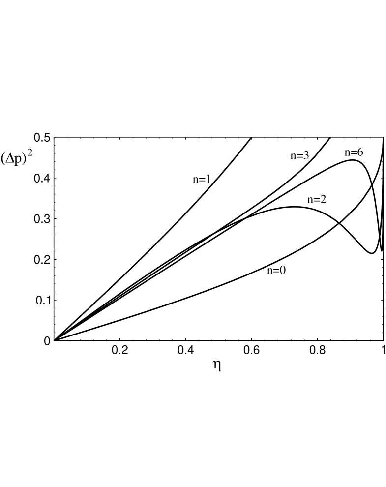
Figure 5: The quadrature uncertainty $(\Delta p)^{2}$ for the $K_{1}$-$K_{2}$ intelligent states versus $\eta$, for different values of $n$.

For $k=1/4$ and $n\geq 2$, $(\Delta p)^{2}$ has a minimum ($\approx 0.25$) for $\delta\approx 1/(2n+1)^{2}$. As $n$ increases, this minimum becomes sharper. We find that even states ($k=1/4$) are squeezed in the whole region $0<\eta<1$, while odd states ($k=3/4$) are squeezed only for sufficiently small values of $\eta$.

According to the properties (2.8) of the intelligent states, we have

$$(\Delta K_{1})^{2}=\frac{\langle K_{3}\rangle}{2\eta}\hskip 22.76228pt(\Delta K_{2})^{2}=\frac{\eta\langle K_{3}\rangle}{2}.$$ (5.70)

For $0<\eta<1$, the generator $K_{2}$ is always relatively squeezed. However, it can be easily verified that absolute quadratic squeezing is impossible for the $K_{1}$-$K_{2}$ ordinary intelligent states.

5.3.4 Eigenstates of $\eta K_{2}+{\rm i}K_{3}$

Here, $\vec{\beta}=(0,\eta,{\rm i})$ and $B={\rm i}\sqrt{\eta^{2}+1}$. The corresponding analytic function is given by equation (4.19) with

$$\tau_{\pm}=\frac{-\eta}{1\pm\sqrt{\eta^{2}+1}}\,.$$ (5.71)

Note that $|\tau_{+}\tau_{-}|=1$. For any $|\eta|<\infty$ there exists $\epsilon>0$ such that $|\tau_{+}|<(1+\epsilon)^{-1}$. Then $|\tau_{-}|>(1+\epsilon)^{-1}$ and the analyticity condition requires that the spectrum is discrete, $\lambda=(k+l)B$. Equation (3.14) shows that these eigenvalues naturally appear in the generation scheme for the $K_{2}$-$K_{3}$ intelligent states. For $\eta=0$, these states reduce to the Fock states $|n\rangle$. For $l=0$, we obtain the SU(1,1) generalized coherent states $|\zeta_{0},k\rangle$ with $\zeta_{0}=-\tau_{+}$.

Since $|\tau_{+}\tau_{-}|=1$, we can use simple expressions (5.27), (5.28) for the moments of the generator $K_{3}$. The parameters used in these expressions are $r=k+l$, $h=(1+\sqrt{\eta^{2}+1})^{2}/\eta^{2}$, $t=4(\eta^{2}+1)/\eta^{2}$, $S_{+}S_{-}=-4/\eta^{2}$. Then we obtain

$$\langle K_{3}\rangle=(k+l)\sqrt{\eta^{2}+1}$$ (5.72)

$$(\Delta K_{3})^{2}=\frac{k\eta^{2}}{2}\left[1+\frac{l+2k}{k}(\eta^{2}+1)\frac{P_{l-1}^{(1,2k)}(2\eta^{2}+1)}{P_{l}^{(0,2k-1)}(2\eta^{2}+1)}\right]\;\;\;\;\;\;\;l\neq 0$$ (5.73)

and $(\Delta K_{3})^{2}=k\eta^{2}/2$ for $l=0$. In deriving equation (5.73) from (5.28), we used the relation $P_{n}^{(\alpha,\beta)}(-x)=(-1)^{n}P_{n}^{(\beta,\alpha)}(x)$. Note also that, by the definition of the eigenstates, $\langle\eta K_{2}+{\rm i}K_{3}\rangle={\rm i}(k+l)\sqrt{\eta^{2}+1}$. This equation gives $\langle K_{2}\rangle=0$ and the expession (5.72) for $\langle K_{3}\rangle$. In the limit $\eta\ll 1$, we find

$$\langle K_{3}\rangle\approx\frac{2n+1}{4}\left(1+\frac{\eta^{2}}{2}\right)\hskip 22.76228pt(\Delta K_{3})^{2}\approx\frac{n^{2}+n+1}{8}\eta^{2}$$ (5.74)

$$g^{(2)}\approx 1-\frac{1}{n}+\frac{2n^{2}+4n+3}{4n^{2}}\eta^{2}\hskip 22.76228ptn\neq 0.$$ (5.75)

Photon statistics is sub-Poissonian in accordance with the fact that for $\eta\rightarrow 0$ the $K_{2}$-$K_{3}$ intelligent states reduce to the Fock states $|n\rangle$. In the limit $\eta\gg 1$, we obtain

$$\langle K_{3}\rangle\approx\frac{2n+1}{4}\eta\hskip 22.76228pt(\Delta K_{3})^{2}\approx\frac{2n+1}{8}\eta^{2}$$ (5.76)

$$g^{(2)}\approx\frac{2n+3}{2n+1}-\frac{2(2n-1)}{(2n+1)^{2}}\frac{1}{\eta}.$$ (5.77)

In this limit photon statistics is super-Poissonian.

According to the properties (2.8) of the intelligent states, we have

$$\langle K_{1}\rangle=\frac{2}{\eta}(\Delta K_{3})^{2}\hskip 22.76228pt(\Delta K_{2})^{2}=\frac{1}{\eta^{2}}(\Delta K_{3})^{2}.$$ (5.78)

Using equation (2.3) for the Casimir operator, one finds

$$\langle K_{1}^{2}\rangle=\langle K_{3}^{2}\rangle-\langle K_{2}^{2}\rangle-k(k-1).$$ (5.79)

Then we obtain

$$(\Delta K_{1})^{2}=\frac{\eta^{2}-1}{\eta^{2}}(\Delta K_{3})^{2}-\frac{4}{\eta^{2}}(\Delta K_{3})^{4}+(k+l)^{2}(\eta^{2}+1)+\frac{3}{16}.$$ (5.80)

The uncertainties of the field quadratures are

$$(\Delta Q_{\pm})^{2}=2(k+l)\sqrt{\eta^{2}+1}\pm\frac{4}{\eta}(\Delta K_{3})^{2}.$$ (5.81)

Since $\eta$ is positive, the condition $(\Delta p)^{2}<(\Delta q)^{2}$ always holds here, and squeezing can be observed only in the $p$ quadrature. In the limit $\eta\ll 1$, we have

$$(\Delta Q_{\pm})^{2}\approx\frac{2n+1}{2}\pm\frac{n^{2}+n+1}{2}\eta+\frac{2n+1}{4}\eta^{2}.$$ (5.82)

In this limit the $p$ quadrature is slightly squeezed only for $n=0$. In the limit $\eta\gg 1$ the $p$ quadrature is strongly squeezed: $(\Delta p)^{2}\rightarrow 0$ as $O(1/\eta)$; while the $q$ quadrature is very noisy: $(\Delta q)^{2}\approx(2n+1)\eta$. Numerical studies show that quadratic squeezing is possible only for the generator $K_{2}$. In the limit $\eta\ll 1$, we have

$$(\Delta K_{1})^{2}\approx(\Delta K_{2})^{2}\approx\frac{n^{2}+n+1}{8}.$$ (5.83)

There is no quadratic squeezing in this limit, except for weak relative squeezing in $K_{2}$ for $n=0$. In the limit $\eta\gg 1$, the generator $K_{1}$ is very noisy, while $K_{2}$ is strongly relatively squeezed:

$$(\Delta K_{1})^{2}\approx\frac{2n+1}{8}\eta^{2}\hskip 22.76228pt(\Delta K_{2})^{2}\approx\frac{2n+1}{8}.$$ (5.84)

Absolute quadratic squeezing is impossible for the $K_{2}$-$K_{3}$ ordinary intelligent states.

6 Conclusions

We have presented a scheme for the generation of the SU(1,1) intelligent states. This scheme employs quantum correlations created in a non-degenerate parametric amplifier between the vacuum and the squeezed vacuum. These quantum correlations (the entanglement) between the two light modes enable us to manipulate the state of one of the modes by a measurement of the photon number in the other. A powerful analytic method has been used for obtaining exact closed expressions for quantum statistical properties of the intelligent states. We have seen that these states can exhibit interesting nonclassical properties of strong antibunching and squeezing. We have found that even states have a tendency to be squeezed, while odd states are more likely to be antibunched.

References

- [1] Jackiw R 1968 J. Math. Phys. 9 339
-
[2]
Aragone C, Guerri G, Salamo S and Tani J L 1974
J. Phys. A: Math. Gen. 7 L149
Aragone C, Chalbaud E and Salamo S 1976 J. Math. Phys. 17 1963 - [3] Vanden-Bergh G and DeMeyer H 1978 J. Phys. A: Math. Gen. 11 1569
- [4] Wodkiewicz K and Eberly J H 1985 J. Opt. Soc. Am. B 2 458
- [5] Nieto M M and Truax D R 1993 Phys. Rev. Lett. 71 2843
- [6] Hillery M and Mlodinow L 1993 Phys. Rev. A 48 1548
-
[7]
Bergou J A, Hillery M and Yu D 1991
Phys. Rev. A 43 515
Yu D and Hillery M 1994 Quantum Opt. 6 37 - [8] Trifonov D A 1994 J. Math. Phys. 35 2297
- [9] Puri R R 1994 Phys. Rev. A 49 2178
- [10] Agarwal G S and Puri R R 1994 Phys. Rev. A 49 4968
- [11] Brif C and Ben-Aryeh Y 1994 J. Phys. A: Math. Gen. 27 8185
- [12] Brif C and Ben-Aryeh Y 1994 Phys. Rev. A 50 3505
-
[13]
Prakash G S and Agarwal G S 1994 Phys. Rev. A
50 4258
Prakash G S and Agarwal G S 1995 Phys. Rev. A 52 2335 -
[14]
Gerry C C and Grobe R 1995 Phys. Rev. A
51 4123
Gerry C C and Grobe R 1997 Quantum Semiclass. Opt. 9 59
Gerry C C, Gou S-C and Steinbach J 1997 Phys. Rev. A 55 630 -
[15]
Brif C and Ben-Aryeh Y 1996 Quantum
Semiclass. Opt. 8 1
Brif C and Mann A 1996 Phys. Lett. 219A 257
Brif C and Mann A 1996 Phys. Rev. A 54 4505 - [16] Puri R R and Agarwal G S 1996 Phys. Rev. A 53 1786
- [17] Luis A and Peřina J 1996 Phys. Rev. A 53 1886
- [18] Brif C 1996 Ann. Phys., N.Y. 251 180
- [19] Brif C 1997 Int. J. Theor. Phys. 36 1677
- [20] Trifonov D A 1996 preprint quant-ph/9609001
- [21] Trifonov D A 1996 preprint quant-ph/9609017
- [22] Trifonov D A 1997 preprint quant-ph/9701018
- [23] Brif C, Vourdas A and Mann A 1996 J. Phys. A: Math. Gen. 29 5873
- [24] Bargmann V 1947 Ann. Math. 48 568
- [25] Bishop R F and Vourdas A 1987 J. Phys. A: Math. Gen. 20 3727
- [26] Hong C K and Mandel L 1986 Phys. Rev. Lett. 56 58
- [27] Yamamoto Y, Mashida S, Imoto M, Kitagawa M and Björk G 1987 J. Opt. Soc. Am. B 10 1645
- [28] Watanabe K and Yamamoto Y 1988 Phys. Rev. A 38 3556
- [29] Holmes C A, Milburn G J and Walls D F 1989 Phys. Rev. A 39 2493
- [30] Agarwal G S 1990 Quantum Opt. 2 1
- [31] Lukš A, Peřinová V and Křepelka J 1994 J. Mod. Opt. 41 2325
-
[32]
Zou X Y, Wang L J and Mandel L 1991
Phys. Rev. Lett. 67 318
Wang L J, Zou X Y and Mandel L 1991 Phys. Rev. A 44 4614
Zou X Y, Grayson T, Barbosa G A and Mandel L 1993 Phys. Rev. A 47 2293 - [33] Kwiat P G, Steinberg A M and Chiao R Y 1994 Phys. Rev. A 49 61
- [34] Perelomov A M 1986 Generalized Coherent States and Their Applications (Berlin: Springer)
- [35] Stoler D 1970 Phys. Rev. D 1 3217; 1971 Phys. Rev. D 4 2308
- [36] Yuen H 1976 Phys. Rev. A 13 2226
- [37] Brif C, Mann A and Vourdas A 1996 J. Phys. A: Math. Gen. 29 2053
- [38] Barut A O and Raczka R 1986 Theory of Group Representations and Applications, 2nd ed (Singapore: World Scientific)
- [39] Erdélyi et al. (ed) 1953 Higher Transcendental Functions: Bateman Manuscript Project (New York: McGraw-Hill)
- [40] Barut A O and Girardello L 1971 Commun. Math. Phys. 21 41
- [41] Dodonov V V, Malkin I A and Man’ko V I 1974 Physica 72 597