Quantum Networking with Optical Fibres

Abstract

I propose a scheme which allows for reliable transfer of quantum information between two atoms via an optical fibre in the presence of decoherence. The scheme is based on performing an adiabatic passage through two cavities which remain in their respective vacuum states during the whole operation. The scheme may be useful for networking several ion–trap quantum computers, thereby increasing the number of quantum bits involved in a computation.

The possibility of reliable spacial transport of quantum states is of crucial importance to quantum communication. During the past few years rapid progress has been made in using optical fibres for quantum communication on the single photon level [1]. This is needed for quantum cryptography [1, 2] and quantum teleportation [3]. However, the spatial exchange of quantum information between quantum registers that have undergone local quantum processing has not yet been demonstrated experimentally. Quantum communication between locally distinct nodes of a quantum network will be essential to overcome small–scale quantum computing [4].

A promising model for storage and local processing of quantum information is the ion–trap quantum computer, in which the quantum bits are stored in stable ground states or in long–lived metastable states [5]. First experimental results have already been reported [6]. However, technology imposes an upper limit on the number of ions, and thus quantum bits, which can be used in a single ion–trap quantum computer. To overcome this limit, a network of several ion trap quantum computers could be set up. But while ions are superb for storing quantum information, it seems more feasible to mediate quantum states by photons carried by optical fibres.

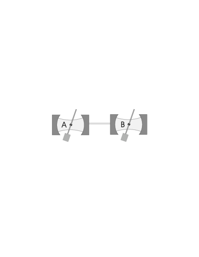
FIG. 1.: Representation of the scheme. The atoms (quantum bits) are coupled to cavities and are manipulated by lasers. The cavities are connected via an optical fibre.

This problem has been recently addressed (to my knowledge, for the first time) by Cirac et al. [7]. They propose a scheme to transmit quantum bits by tailoring time–symmetric photon wave–packets. In the present letter, I will pursue a different approach which is based on an adiabatic passage via photonic dark states. A representation of the scheme is depicted in Fig. 1.

The quantum bit to be transferred is initially stored in atom A, and atom B is prepared in a predefined state. Atoms A and B may be part of ion–trap quantum computers. Initially both cavities and the fibre are in the vacuum state. By appropriate design of laser pulses as described below we may swap the states of atom A and B. Below I will demonstrate that (ideally) the two cavities will never have a photon number different from zero.

The scheme has two distinctive features: Firstly, it is insensitive to losses from the cavities into other than the fibre modes. This is due to the fact that the cavities are never populated. As a result, the coupling between the cavities and the fibre mode does not need to be perfect; Secondly, it does not require a precise control of the pulse shape, duration and intensity of the manipulating laser pulses is not required as long as some “global” (namely adiabaticity–) conditions are met. This implies that the Rabi frequencies need not be known in order to perform the transfer successfully.

The individual atom–cavity systems are described as follows. The atoms are modelled by three–level $\Lambda$–systems with two ground states $|a_{0}\rangle$, $|a_{1}\rangle$ and one excited state $|b\rangle$ as depicted in Fig. 2a.

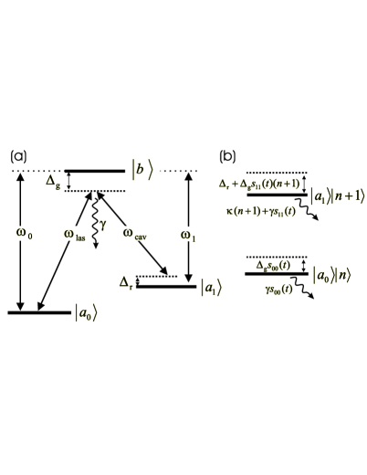
FIG. 2.: (a) Atomic level scheme. See text for definition of the symbols. (b) Level scheme of the combined atom–cavity system after adiabatic elimination. The first parameter in the ket represents an atomic ground state whereas the second parameter denotes a cavity mode Fock state.

The frequency of the transition $|a_{i}\rangle-|b\rangle$ is denoted by $\omega_{i}$, where $i=0,1$. The excited state $|b\rangle$ spontaneously decays with a rate $\gamma$. The cavity is modelled by a single, quantized mode with frequency $\omega_{\rm cav}$ coupled to the transition $|a_{1}\rangle-|b\rangle$ with coupling strength $g$. The cavity is coupled to an optical fibre as described below. In addition, we include a loss rate $\kappa$ of the cavity. This decay rate includes any undesired loss mechanisms such as absorption of cavity photons in the mirrors and coupling to other than the fibre modes. The transition $|a_{0}\rangle-|b\rangle$ is coupled to a laser described by a c–number coherent field with frequency $\omega_{\rm las}$. The corresponding time–dependent Rabi frequency is denoted by $\Omega(t)$. According to continuous measurement theory the evolution of a system in the absence of quantum jumps is determined by an effective, non–Hermitian Hamiltonian [8]. In the present context we find:

$$H_{\rm eff} = H_{0}+H_{\rm int}$$ (1)

$$H_{0} = (-\Delta_{\rm g}-i\gamma)|b\rangle\langle b|+\Delta_{\rm r}|a_{1}\rangle\langle a_{1}|+\kappa a^{\dagger}a$$ (2)

$$H_{\rm int} = \Omega(t)|b\rangle\langle a_{0}|+ga|b\rangle\langle a_{1}|+H.c.$$ (3)

Eq. (1) is written in a rotating frame. The symbols $a$ and $a^{\dagger}$ denote the annihilation and creation operators of the cavity mode. Here I have introduced two detunings, namely the “global” detuning $\Delta_{\rm g}=\omega_{\rm las}-\omega_{0}$ and the “Raman” detuning $\Delta_{\rm r}=(\omega_{\rm cav}-\omega_{\rm las})-(\omega_{0}-\omega_{1})$.

We are interested in the low saturation regime where we can adiabatically eliminate the excited atomic state. Below the conditions that are required to make this approximation meaningful are given. By applying standard quantum optical techniques [9] the adiabatically eliminated effective Hamiltonian reads:

$$\tilde{H}_{\rm eff} = \tilde{H_{0}}+\tilde{H_{1}}+\tilde{H}_{\rm int}$$ (4)

$$\tilde{H}_{0} = +\left(\Delta_{\rm g}s_{00}(t)-i\gamma s_{00}(t)\right)|a_{0}\rangle\langle a_{0}|$$ (5)

$$\tilde{H_{1}} = \left(\Delta_{\rm r}+\Delta_{g}s_{11}(t)a^{\dagger}a-i\kappa a^{\dagger}a-i\gamma s_{11}(t)\right)|a_{1}\rangle\langle a_{1}|$$ (6)

$$\tilde{H}_{\rm int} = \left(\Delta_{g}-i\gamma\right)s_{01}(t)a|a_{0}\rangle\langle a_{1}|+$$ (8)

$$\left(\Delta_{g}-i\gamma\right)s_{10}(t)a^{\dagger}|a_{1}\rangle\langle a_{0}|.$$

Here I have introduced the saturation parameters

$$s_{00}(t) = \frac{|\Omega(t)|^{2}}{\Delta_{\rm g}+\gamma^{2}}\quad\quad s_{11}(t)=\frac{|g|^{2}}{\Delta_{\rm g}^{2}+\gamma^{2}}$$ (9)

$$s_{01}(t) = s_{10}^{*}(t)=\frac{\Omega(t)g^{*}}{\Delta_{\rm g}^{2}+\gamma^{2}}.$$ (10)

Adiabatic elimination is applicable if the following inequalities hold:

$\displaystyle s_{ii}(t)\ll 1,\quad i=1,2.$

The detunings, light–shifts, and decay rates of the two ground states are shown in Fig. 2b. In Eq. (4), $\tilde{H_{0}}$ and $\tilde{H}_{1}$ contain all the terms which are diagonal in the atomic basis. Both ground states undergo light shifts and damping. Later we will find that the light shift of state $|a_{0}\rangle$ gives rise to undesired effects which will make compensate necessary. $\tilde{H}_{\rm int}$ describes Rabi oscillations between the ground states and contains dissipative terms as well. The decay terms are of course unwanted. However, it will be shown in the following how they can be avoided.

The next step is to consider two atom–cavity systems as described above connected by an optical fibre. The free Hamiltonian of the fibre and the interaction Hamiltonian with the two atom–cavity systems is assumed to take the following form:

$$H_{\rm fib}=\sum_{k}\Delta_{k}f_{k}^{\dagger}f_{k}+\left\{\nu\sum_{k}\left(a_{A}+(-1)^{k}a_{B}\right)f_{k}+H.c.\right\}$$ (11)

Eq. (11) is written in a frame rotating at the cavity frequency. By $f_{k}(f_{k}{\dagger})$ I denote the annihilation (creation) operator of the $k$th fibre mode. $\Delta_{k}$ is the frequency difference between the $k$th fibre mode and the cavity mode, and $\nu$ is the coupling strength between the fibre modes and the cavity. For simplicity it is assumed that in the frequency range where the coupling is significant the coupling strength is constant. Here, and in the remainder of this letter, the subscripts (or superscripts) $A$ and $B$ distinguish the two atom–cavity sub–systems. Note that the fibre is assumed to be lossless which is of course unrealistic for long transmission distances. However, the present scheme is designed for short distances for which this assumption seems appropriate.

The goal is to achieve quantum state swapping. In this model energy eigenstates of the system and logical values are identified as follows:

$\displaystyle|i\rangle|j\rangle\equiv|a_{i},0\rangle_{A}|a_{j},0\rangle_{B}|{\rm vac}\rangle\quad\quad i=0,1$

Here the first and the second ket on the right hand side refer to the atom–cavity subsystem $A$ and $B$. The first parameter in each ket denotes the atomic ground state, while the second represents a Fock state of the respective cavity modes. The third ket denotes the subsystem of the fibre–modes all being in the vacuum state. Below I will demonstrate how the following operation can be performed:

$$\left(\alpha|0\rangle+\beta|1\rangle\right)|1\rangle\longrightarrow|1\rangle\left(\alpha|0\rangle+\beta|1\rangle\right).$$ (12)

Heree $\alpha$ and $\beta$ are arbitrary (in general unknown) complex amplitudes. The result of the process by starting with the second quantum bit in state $|0\rangle$ will be undefined.

The primary objective is to perform the desired quantum state transfer with as little disturbing influence from dissipative processes as possible. In the present context these are spontaneous emissions from the atomic excited states (via optical pumping) and the decay of the cavity mode into other than the fibre–modes. These two decay mechanisms are dealt with as follows: (i) The optical pumping rate is the product of the saturation parameter $s_{ii}(t)$ and the spontaneous decay rate $\gamma$, whereas the effective Rabi frequency is the product of $s_{01}(t)$ and the detuning $\Delta_{g}$. Therefore, by increasing the detuning and simultaneously increasing the Rabi frequency the optical pumping rate can be made arbitrarily small while maintaining the effective Rabi frequency constant. (ii) Undesired loss of cavity photons is avoided by performing the process as an adiabatic passage through a dark state of both cavities. In other words, the photon number of two cavity modes will not differ significantly from zero throughout the whole process. In the following paragraphs I will elaborate on the details of this scheme.

Adiabatic passage [10] has a variety of applications in the context of atomic physics. For example, it can be used for transferring population between atomic levels unaffected by spontaneous emission [11]. A beam splitter for atoms based on adiabatic passage has been proposed by Marte et al. and realized experimentally by several groups [12]. Moreover, in cavity QED quantum state sythesis [13] and quantum computing [14] based on adiabatic passage has been proposed.

Since spontaneous emission can be dealt with in the aforementioned way we will set $\gamma=0$ in the following. The present scheme is based on the fact that for the Hamiltonian $H_{\rm part}=\tilde{H}_{1}+\tilde{H}_{\rm int}+\tilde{H}_{\rm fib}$ given in Eqs. (4) and (11) dark states with respect to the two cavity modes exists. This requires that a fibre mode exists that is resonant with the cavity mode, i.e. that a detuning $\Delta_{k}=0$ for a certain $k$ exists. Note that this is not the full Hamiltonian of the system since $\tilde{H}_{0}$ is missing. It turns out that $\tilde{H}_{0}$ deteriorates the dark state and thus the performance of the scheme. Below it will be shown how this effect can be avoided. The two relevant dark states of the partial Hamiltonian $H_{\rm part}$ read thus:

$$|\Psi^{D}_{0}\rangle \propto \nu\Delta s_{10}^{B}(t)|a_{0},0\rangle_{A}|a_{1},0\rangle_{B}|\rm vac\rangle$$ (15)

$$-\Delta^{2}s_{10}^{A}(t)s_{10}^{B}(t)|a_{1},0\rangle_{A}|a_{1},0\rangle_{B}|1_{k_{0}}\rangle$$

$$+\nu\Delta s_{10}^{A}(t)|a_{1},0\rangle_{A}|a_{0},0\rangle_{B}|\rm vac\rangle$$

$$|\Psi^{D}_{1}\rangle = |a_{1},0\rangle_{A}|a_{1},0\rangle_{B}|\rm vac\rangle.$$ (16)

By $|1_{k_{0}}\rangle$ I denote the fibre state corresponding to fibre mode $k_{0}$ being in a one photon Fock state and all the others in the vacuum state. The index $k_{0}$ corresponds to the fibre mode for which $\Delta_{k_{0}}=0$. These states are eigenstates of $H_{\rm part}$ and do not contain excited states of the cavity mode. In the first dark state $|\Psi^{D}_{0}\rangle$ the cavity modes are not populated due to destructive quantum interference, whereas the second dark state $|\Psi^{D}_{1}\rangle$ is decoupled from the laser interaction in a trivial way.

The central idea is to use this dark state for adiabatic passage. If the system is prepared in the above dark state (15) and the laser intensities are changed slowly (i.e. adiabatically) no other eigenstates of $H_{\rm part}$ will be populated. Therefore, throughout the whole process the two cavity modes will not be populated. In our particular case we initially have an unknown quantum superposition prepared in subsystem $A$ as given in Eq. (12). This initial state can in fact be written as a superposition of the two dark states $|\Psi^{D}_{0,1}\rangle$ provided that $s_{10}^{B}(t)\gg s_{10}^{A}(t)$:

$\displaystyle\left(\alpha|0\rangle+\beta|1\rangle\right)|1\rangle=\alpha|\Psi^{D}_{0}\rangle+\beta|\Psi^{D}_{1}\rangle$

In practice this means that at the beginning of the transfer the laser which acts on the atom in subsystem $B$ is switched on first. During the transfer the laser intensities are changed such that at the end the inequality $s_{10}^{B}(t)\ll s_{10}^{A}(t)$ holds. If the change is carried out slowly enough the system at the end is still the above superposition of $|\Psi^{D}_{0}\rangle$ and $|\Psi^{D}_{1}\rangle$. However, this quantum state now corresponds to the desired final state of the transfer, i.e.

$\displaystyle\alpha|\Psi^{D}_{0}\rangle+\beta|\Psi^{D}_{1}\rangle=|1\rangle\left(\alpha|0\rangle+\beta|0\rangle\right).$

An important feature of the scheme is that the details of the laser pulses are not important as long as the process is carried out adiabatically.

As mentioned above, the Hamiltonian ${H}_{\rm part}$ is not the total Hamiltonian of the system because it does not contain $\tilde{H}_{0}$ specified in Eq. (4). This Hamiltonian contains light shift of the state $|a_{0}\rangle$ which will destroy the dark state Eq. (15). However, this light shift can be compensated for quite straightforwardly by using a second laser which couples the atomic level $|a_{0}\rangle$ non–resonantly with an additional level further up in the atomic level scheme. The intensity of this laser is chosen such that the total light shift of $|a_{0}\rangle$ adds up to zero.

In the remainder of this letter I will present numerical results in order to evaluate the performance of the scheme. Note that the coupling strength $\nu$ will decrease when the length of the fibre is increased. Therefore, it is advantageous to introduce a coupling strength per unit length defined as:

$\displaystyle\alpha=\nu\sqrt{L},$

where $L$ is the length of the fibre. We shall express all the other parameters in units of $\alpha$, and a unit length $L_{0}$. The order of magnitude of $\alpha$ in terms of known quantities can be estimated as follows. Suppose the fibre is infinitely long and the decay rate of the single cavity mode into the continuum of fibre modes is $\kappa_{f}$. As a result of the quantum fluctuation–dissipation theorem the coupling strength between the cavity mode and the output–field of the fibre modes is $g_{f}=\sqrt{2\kappa_{f}}$ [9]. Now we estimate the coupling of the cavity mode to the individual fibre modes provided that $L$ is finite. Let us first estimate the number of fibre modes which are coupled to the cavity mode. For simplicity we assume that the mode separation between neighboring fibre modes to be $4\pi c/L$, where $c$ denotes the speed of light. This means that the number of fibre modes which couple significantly to the cavity mode is of the order of $N=\kappa_{f}L/4\pi c$. We can estimate the coupling of the cavity mode to an individual fibre mode by multiplying $g_{f}$ by a factor which reflects the discretization of the spectrum. From the commutation relations of the field operators we conclude that this factor fulfills the following relation:

$\displaystyle f\approx\sqrt{\kappa_{f}/N}.$

Thus the coupling of the cavity mode to an individual fibre mode is approximately:

$\displaystyle\nu=\alpha/\sqrt{L}\approx\sqrt{8\kappa_{f}\pi c/L}.$

As a concrete numerical example let us assume that the decay rate of the fibre into the cavity is $\kappa/2\pi=0.5{\rm GHz}$. Thus we find $\alpha/2\pi\approx 0.8{\rm GHz}\sqrt{m}$. Moreover, suppose the unwanted cavity loss rate is $\kappa/2\pi=100{\rm MHz}$. In units of $\alpha$ the cavity loss rate and the mode detuning are $\kappa\approx 0.13{\rm m}^{-1/2}\alpha$ and $\Delta_{k}\approx(k/L)0.77{\rm m}^{-1/2}\alpha$. We will find later that reliable transfer can be achieved in principle for a transfer time of the order of $t\approx 300{\rm m}^{1/2}\alpha^{-1}\approx 60{\rm ns}$.

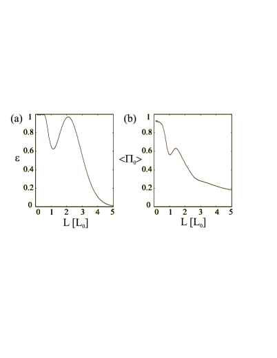
FIG. 3.: (a) Population in the quantum state $|a_{1},0\rangle|a_{0},0\rangle|vac\rangle$$\equiv$$|1\rangle|0\rangle$ after the transfer (initial state $|a_{0},0\rangle|a_{1},0\rangle|vac\rangle$ $\equiv$$|0\rangle|1\rangle$) against the length of the fibre in units of $L_{0}$. The total time of the transfer was chosen as $T$$=$$300$ $\alpha$ $L_{0}^{1/2}$. The pulse shape of the two lasers was assumed to be Gaussian: $\Delta_{g}s_{01}^{A,B}(t)$ $=$ $c{\rm exp}$ $\left(-(t-t_{A,B})^{2}/w^{2}\right)$, with $c=2\alpha L_{0}^{-1/2}$, $t_{B}-t_{A}=0.2T$ and $w=0.05T$. The scaled cavity loss rate and the separation between neighbor fibre modes were chosen as $\kappa=0.1\alpha L_{0}^{-1/2}$ and $\Delta=0.1\alpha L_{0}^{-1/2}$, respectively. (b) The time average of the expectation value of the photon number in the resonant, dark fibre mode divided by the time–average of the expectation value of the total photon number in the fibre. The parameters are the same as in (a).

In Fig. 3a the performance of the scheme is studied as a function of the length of the fibre. A good measure is the population $\varepsilon$ in the quantum state $|a_{1},0\rangle|a_{0},0\rangle|vac\rangle\equiv|1\rangle|0\rangle$ after the transfer for an inital state $|a_{0},0\rangle|a_{1},0\rangle|vac\rangle\equiv|0\rangle|1\rangle$. As pointed out earlier the state $|a_{1},0\rangle|a_{1},0\rangle|vac\rangle\equiv|1\rangle|1\rangle$ is decoupled from the laser interaction and thus remains unchanged. The length $L$ of the fibre is plotted in units of $L_{0}$. For small values of $L$ the transfer is almost perfect. As the length of the fibre is increased the population $\varepsilon$ decreases (after going through a local maximum) and thus the performance of the scheme deteriorates. This behaviour is due to the fact that the distance between neighbor modes decreases with increasing fibre length. Therefore, more and more “grey” states (i.e. states which are not perfectly dark) in the neighborhood of the resonant dark state are involved in the transfer. Note that this asymptotic behaviour is required for causality reasons. If all the modes besides the central mode are neglected a transfer between the nodes could take place in constant time regardless of the length of the fibre.

Finally, in Fig. 3b I show to what extent the dark state Eq. (15) is populated during the transfer. We plot $\langle\Pi_{0}\rangle$, the average population in the dark state divided by the average total photon number within the fibre. Surprisingly, rather good transfer can be found even in the case where $\langle\Pi_{0}\rangle$ is not close to one. This suggests that a significant portion of the population passes through non–dark states in the neighborhood of the dark state and very good transfer can take place for parameters where the single mode approximation of the fibre is not at all valid.

In summary, I have proposed a novel scheme to transfer quantum states between distant nodes of a quantum network which is robust against important sources of decoherence. The scheme could be used to enable networking of several ion trap quantum computers. In addition, error correction methods could be applied to further increase the stability of the scheme [15, 16].

I wish to acknowledge fruitful discussions with Artur Ekert, the members of the quantum information group at Oxford University, and Jonathan Roberts. The author holds an Erwin–Schrödinger scholarship granted by the Austrian Science Fund.

REFERENCES

- [1] Zbinden et al., Electronics Lett. 33, 586 (1997); C. Marand and P. D. Townsend, Opt. Lett. 20, 1695 (1995); R. J. Hughes et al., Contemp. Phys. 36, 149 (1995).
- [2] S. Wiesner, SIGACT News 15, 78 (1983); C. H. Bennet and G. Brassard, Proceedings of the IEEE Intl. Conf. on Computers, Systems and Signal Processing, Bangalore (New York, IEEE, 1984).
- [3] C. H. Bennet et al., Phys. Rev. Lett 70, 1895 (1993).
- [4] A. Ekert, Proc. 14th International Conference on Atomic Physics ICAP, ed. Smith S., Wieman C., Wineland D., 450, American Institute of Physics, New York (1995); C. Bennett, Phys. Today 48(10), 24 (1995); D. P. DiVincenzo, Science 270, 255 (1995); S. Lloyd, Sci. Am. 273(4), 44 (1995).
- [5] J. I. Cirac and P. Zoller, Phys. Rev. Lett. 74, 4091 (1995).
- [6] C. Monroe et al., Phys. Rev. Lett. 75, 4714 (1995).
- [7] J. I. Cirac, P. Zoller, H. J. Kimble, and H. Mabuchi, Phys. Rev. Lett. 78, 3221 (1997).
- [8] P. Zoller and C. W. Gardiner, in Proceedings of the Les Houches Lecture Session LXII: Quantum Fluctuations, ed. E. Giacobino and S. Renaud, North Holland, Amsterdam (1996).
- [9] C. W. Gardiner, Quantum Noise (Springer–Verlag, Berlin 1991).
- [10] J. Oreg, F. T. Hioe, and J. H. Eberly, Phys. Rev. A 29, 690 (1984).
- [11] B. W. Shore et al., Phys. Rev. A 44, 7442 (1991).
- [12] P. Marte, P. Zoller, and J. L. Hall, Phys. Rev. A 44, R4118 (1991); L. S. Goldner et al., Phys. Rev. Lett. 72, 997 (1994); J. Lawall and M. Prentiss, Phys. Rev. Lett. 72, 993 (1994).
- [13] A. S. Parkins et al., Phys. Rev. Lett. 71, 3095 (1993).
- [14] T. Pellizzari, S. A. Gardiner, J. I. Cirac, and P. Zoller, Phys. Rev. Lett. 75, 3788 (1995).
- [15] S. J. van Enk, J. I. Cirac, and P. Zoller, Phys. Rev. Lett. 78, 4293 (1997).
- [16] J. I. Cirac, T. Pellizzari and P. Zoller, Science 273, 5279 (1996).