Effective Pure States for Bulk Quantum Computation

Abstract

In bulk quantum computation one can manipulate a large number of indistinguishable quantum computers by parallel unitary operations and measure expectation values of certain observables with limited sensitivity. The initial state of each computer in the ensemble is known but not pure. Methods for obtaining effective pure input states by a series of manipulations have been described by Gershenfeld and Chuang [1, 2] (logical labeling) and Cory et al. [3, 4] (spatial averaging) for the case of quantum computation with nuclear magnetic resonance. We give a different technique called temporal averaging. This method is based on classical randomization, requires no ancilla qubits and can be implemented in nuclear magnetic resonance without using gradient fields. We introduce several temporal averaging algorithms suitable for both high temperature and low temperature bulk quantum computing and analyze the signal to noise behavior of each.

I Introduction

Quantum computation involves the transformation of one known pure quantum state into another unknown state, which can be measured to provide a computationally useful output. Traditionally, it has been understood that an important part of this process is proper preparation of a fiducial initial pure state, such that the computational input is well known, and the output is thus meaningful. In particular, it has usually been assumed that the input cannot be a stochastic mixture. However, two groups[1, 2, 3, 4] have recently shown that by using a different technique, called bulk quantum computation, the same computation can be performed but with an initial mixture state, which is often much easier to achieve experimentally. Bulk quantum computation is being implemented for small numbers of qubits using nuclear magnetic resonance (NMR) techniques.

Bulk quantum computation is performed on a large ensemble of indistinguishable quantum computers. At the beginning of a computation, each member $c$ of the ensemble is in an initial state $\rho_{c,0}$ such that the average $\rho_{0}\doteq\mbox{Exp}(\rho_{c,0})$ of these states is known. A bulk computation with such an ensemble can be divided into three steps consisting of preparation, computation and readout. Each of these steps is equivalent to an application of the same quantum operation to each member of the ensemble. The purpose of the preparation step is to transform the input state to an effective pure state which permits an unbiased observation of the output of the algorithm. The computation is assumed to be a fixed unitary operator derived from a standard quantum algorithm, that is an algorithm with a one qubit answer. We wish to determine this answer on input ${|\mbox{\bf 0}\rangle}$ (the state where every qubit is ${|0\rangle}$). The readout procedure may include some postprocessing of the algorithm’s output and terminates in the measurement of the observable $\sigma_{z}^{(1)}$, the spin along the $z$-axis of the first qubit. In bulk quantum computation, the measurement yields a noisy version of the average value of $\sigma_{z}^{(1)}$ over the ensemble of quantum computers. For our signal to noise analyses, we assume that the noise is unbiased with variance $s^{2}$.

Formally, a bulk quantum computation of an algorithm implementing the unitary transformation $C$ with preparation and postprocessing operations ${\cal P}$ and ${\cal R}$ transforms $\rho_{0}$ to

$$\rho_{out} = \sum_{i,j}R_{i}CP_{j}\rho_{0}P_{j}^{\dagger}C^{\dagger}R_{i}^{\dagger},$$ (1)

where the $R_{i}$ and $P_{j}$ are the operators in a linear representation of the quantum operations ${\cal P}$ and ${\cal R}$ [5]. The measurement step of the readout procedure yields $\mbox{tr}(\rho_{out}\sigma_{z}^{(1)})$ with noise. In the methods investigated in this paper, ${\cal R}$ is unitary, usually the identity. The purpose of ${\cal P}$ is to create an effective pure state. The simplest example of an effective pure state is a density matrix of the form

$$\sum_{j}P_{j}\rho_{0}P_{j}^{\dagger} = p\,{|0\rangle}{\langle 0|}+{q\over N}I.$$ (2)

Here $N=\dim(I)=2^{n}$, where $n$ is the number of qubits. If ${\cal R}=I$, then $\rho_{out}=pC{|\mbox{\bf 0}\rangle}{\langle\mbox{\bf 0}|}C^{\dagger}+{1\over N}I$, so that

$$\mbox{tr}(\rho_{out}\sigma_{z}^{(1)}) = p\ \mbox{tr}(C{|\mbox{\bf 0}\rangle}{\langle\mbox{\bf 0}|}C^{\dagger}\sigma_{z}^{(1)}).$$ (3)

If the excess probability $p$ of the ground state ${|\mbox{\bf 0}\rangle}$ is larger than the smallest detectable signal, we are able to determine whether the output of a standard algorithm is $0$ or $1$ by learning whether the measurement yields a negative or a positive value. To achieve sufficient confidence in the answer or to learn more about the average answer, the bulk computation is repeated several times. Confidence $c$ in the answer of a standard algorithm at a signal to noise ratio of SNR per experiment requires $\sim\log(1/c)/\mbox{SNR}^{2}$ experiments.

Prior to the present work, there were two approaches to implementing an effective pure state preparation procedure. These approaches may be classified as spatial averaging and logical labeling. Spatial averaging was introduced and implemented by Cory et al. [3, 4]. In general, spatial averaging involves partitioning the ensemble of quantum computers into a number of subensembles and applying a different unitary operator to each of them. Given enough subensembles and proper choices of unitary operators, the average density matrix over the whole ensemble can be transformed into an effective pure state. This procedure requires methods for distinguishing between quantum computers in the ensemble. In NMR this can be accomplished by using well-known gradient pulse methods to address individual cells in a bulk sample. The cells in the implementation of Cory et al. are two dimensional slices of constant magnetic fields defined by a transient gradient. The logical labeling technique of Gershenfeld and Chuang [1, 2] is fundamentally different; it avoids the use of explicit subensembles by exploiting ancillary qubits as labels. An initial unitary transformation is applied which redistributes the states in such a way that conditional on the state of the labels, an effective pure state is obtained in the qubits to be used for computation. Gershenfeld and Chuang demonstrated that this can be done efficiently in the high temperature limit for non-interacting qubits, where $\rho_{0}$ can be expressed as a small deviation from ${1\over N}I$.

Here, we consider a new and different technique: Temporal averaging. Rather than attempting to guarantee an effective pure state in a single experiment, this method uses several experiments with different preparation steps chosen either systematically or randomly. The measurements from each experiment are averaged to give the final answer. The preparation steps are chosen such that the average of the prepared input states is an effective pure state. The advantages of this method are that no ancillary qubits are needed, it can be implemented to work at any temperature and it is not necessary to distinguish subensembles of quantum computers. In the high temperature regime it can be implemented efficiently without any loss of signal, and in general, the signal to noise ratios are sufficiently well behaved to permit efficient determination of the desired answer to any given level of confidence.

We will describe several temporal averaging methods and discuss their properties. Temporal averaging methods can be loosely categorized into high temperature and low temperature methods. The high temperature methods tend to be simpler and are the most efficient for NMR quantum computations involving small numbers of qubits. Three such methods will be described: Exhaustive averaging, labeled flip&swap and randomized flip&swap. Labeled flip&swap uses a limited form of logical labeling to obtain the desired answer in two experiments with only one ancilla, while randomized flip&swap needs no ancillas but may require additional experiments to overcome noise from the randomization procedure. Flip&swap methods rely on an inversion symmetry of high temperature thermal states of non-interacting particles. Low temperature methods do not require special assumptions on the initial state, but tend to use more operations to implement. Two such methods are of interest, randomization over a group and averaging by entanglement. The first depends on which unitary group is used. We will show that there are groups which yield good signal to noise behavior and which can be implemented in cubic time. Averaging by entanglement has the advantage of requiring fewer experiments, but necessitates discarding some of the qubits. This method may be useful if some of the qubits are discarded anyway for the purpose of polarization enhancement by computational cooling, a family of techniques for statically or dynamically increasing polarization of the ground state for a subset of the available qubits.

The different temporal averaging methods are introduced and analyzed in the following sections. We begin with a simple example borrowed from NMR, discuss exhaustive averaging and the flip&swap methods, show how randomized averaging over a group can be used and give the method based on entanglement. More detailed descriptions of the algorithms and the mathematical analyses are in the appendix. It is assumed that the reader is familiar with the basic concepts of quantum computation [6, 7, 8] and nuclear magnetic resonance [9].

II NMR Example

To illustrate the ideas on which temporal averaging is based, consider a two qubit example from room temperature NMR with liquids. The density matrix of an AX system consisting of a proton and a carbon-13 nucleus in a 400MHz spectrometer is approximately given by

$$\rho=\frac{1}{4}\left[\begin{array}[]{cccc}1&0&0&0\\ 0&1&0&0\\ 0&0&1&0\\ 0&0&0&1\end{array}\right]+10^{-5}\left[\begin{array}[]{cccc}1&0&0&0\\ 0&0.6&0&0\\ 0&0&-0.6&0\\ 0&0&0&-1\end{array}\right].$$ (12)

How to calculate these input states will be discussed below. Because all relevant observables are traceless, we focus our attention on the second matrix, the deviation density matrix. Suppose our goal is to perform some computation $C$ on the ground state ${|00\rangle}{\langle 00|}$ and then to observe $\sigma_{z}$ on the proton. For this observation, the states ${|01\rangle}{\langle 01|}$, ${|10\rangle}{\langle 10|}$ and ${|11\rangle}{\langle 11|}$ constitute noise. To remove this noise we can exploit the fact that the computation and the observation are linear in the input. We perform three experiments, each with a different preparation step which permutes the undesirable input states, and then average the output. The first experiment uses the unmodified input, corresponding to preparation with $P_{0}=I$. The second permutes ${|01\rangle}{\langle 01|}\rightarrow{|10\rangle}{\langle 10|}\rightarrow{|11\rangle}{\langle 11|}\rightarrow{|01\rangle}{\langle 01|}$ using the unitary transformation

$$P_{1} = \left[\begin{array}[]{cccc}1&0&0&0\\ 0&0&1&0\\ 0&0&0&1\\ 0&1&0&0\end{array}\right].$$ (17)

This results in the input state

$$\rho_{1}=P_{1}\rho P_{1}^{\dagger}=\frac{1}{4}\left[\begin{array}[]{cccc}1&0&0&0\\ 0&1&0&0\\ 0&0&1&0\\ 0&0&0&1\end{array}\right]+10^{-5}\left[\begin{array}[]{cccc}1&0&0&0\\ 0&-0.6&0&0\\ 0&0&-1&0\\ 0&0&0&0.6\end{array}\right].$$ (26)

The third preparation applies the inverse permutation $P_{2}=P_{1}^{\dagger}$ to produce the input state

$$\rho_{2}=P_{2}\rho P_{2}^{\dagger}\frac{1}{4}\left[\begin{array}[]{cccc}1&0&0&0\\ 0&1&0&0\\ 0&0&1&0\\ 0&0&0&1\end{array}\right]+10^{-5}\left[\begin{array}[]{cccc}1&0&0&0\\ 0&-1&0&0\\ 0&0&0.6&0\\ 0&0&0&-0.6\end{array}\right].$$ (35)

The average of the input density matrices is then given by

$$\bar{\rho} = \frac{1}{3}\sum_{i}P_{i}\rho P_{i}^{\dagger}$$ (36)

$$= \frac{1}{4}\left[\begin{array}[]{cccc}1&0&0&0\\ 0&1&0&0\\ 0&0&1&0\\ 0&0&0&1\end{array}\right]+10^{-5}\left[\begin{array}[]{cccc}1&0&0&0\\ 0&-0.333&0&0\\ 0&0&-.333&0\\ 0&0&0&-.333\end{array}\right]$$ (45)

$$= (\frac{1}{4}-0.333\cdot 10^{-5})\left[\begin{array}[]{cccc}1&0&0&0\\ 0&1&0&0\\ 0&0&1&0\\ 0&0&0&1\end{array}\right]+10^{-5}\left[\begin{array}[]{cccc}1.333&0&0&0\\ 0&0&0&0\\ 0&0&0&0\\ 0&0&0&0\end{array}\right].$$ (54)

The average of the measurements of $\sigma_{z}^{(1)}$ after a computation gives $\mbox{tr}(C\bar{\rho}C^{\dagger}\sigma_{z}^{(1)})=1.333\cdot 10^{-5}\mbox{tr}(C{|00\rangle}{\langle 00|}C^{\dagger}\sigma_{z}^{(1)})$. It can be seen that the contributions to the measurements of the undesirable input states have been eliminated. In NMR, $\sigma_{z}^{(1)}$ is measured by applying a radiofrequency pulse to rotate the magnetization of the target spin into the plane and observing the free induction decay as discussed in [2].

III Exhaustive Averaging

The example of the previous section is an instance of exhaustive averaging. For $n$ qubits, it involves cyclicly permuting the non-ground states in $2^{n}-1$ different ways such that the average of the prepared states is given by $(\rho_{00}-\bar{p}){|\mbox{\bf 0}\rangle}{\langle\mbox{\bf 0}|}+\bar{p}I$. This method works for any initial state which is diagonal in the computational basis states. Although the number of experiments required grows exponentially, it is reasonable to consider implementing it for small numbers of qubits.

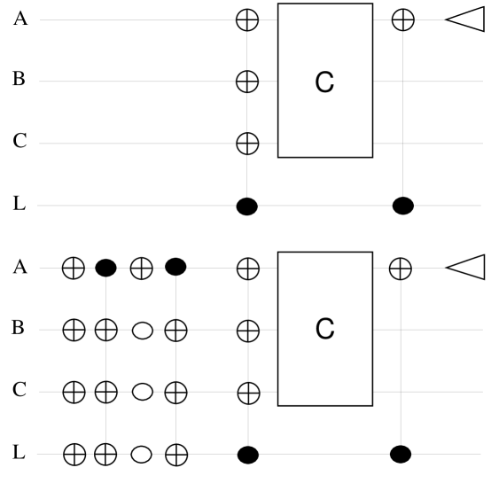
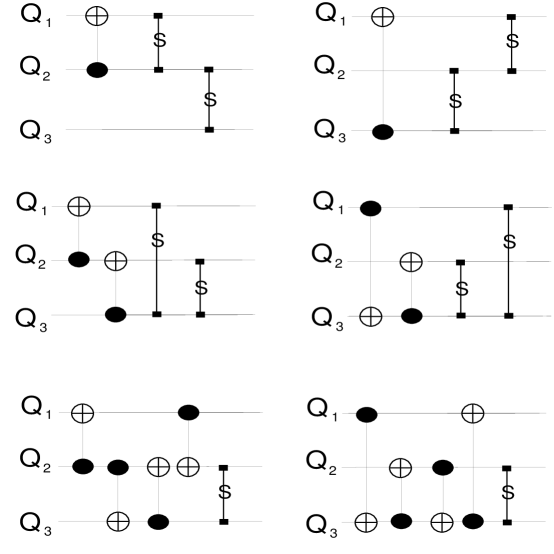
To design the quantum network for the preparation steps, one can exploit the structure of the Galois field $\mbox{GF}(2^{n})$. If the non-ground initial states are labeled by elements of $\mbox{GF}(2^{n})$, multiplication by a non-zero element $x$ of this field implements one of the cyclic permutations. Since multiplication can be implemented with a reasonable (quadratic) number of controlled nots, each such $x$ yields a preparation operator $P_{x}$. Details are given in the appendix. The seven networks needed to exhaustively average three qubits are in Figure 1.

FIG. 1.: Networks required for state preparation when implementing exhaustive averaging for three qubits using controlled-nots and swaps. The networks shown perform the six non-identity cyclic permutations. Seven experiments are performed, one with no special preparation and six with the preparation networks above. $\oplus$ symbols denote the target qubits of the controlled-not gates, and $\bullet$ symbols denote the control.

The signal to noise ratio of exhaustive averaging is determined by the sensitivity of each measurement, the excess probability in the ground state and the number of experiments being performed. If the initial density matrix is $\rho=\sum_{i}\rho_{ii}{|i\rangle}{\langle i|}$ with $0\leq i\leq 2^{n}-1$, then the average density matrix over all experiments is given by $\bar{\rho}=(\rho_{00}-\bar{p}){|0\rangle}{\langle 0|}+\bar{p}I$, where $\bar{p}={1\over 2^{n}-1}\sum_{i=1}^{2^{n}-1}\rho_{ii}$. If the computation’s output is $x=\mbox{tr}(C{|0\rangle}{\langle 0|}C^{\dagger}\sigma_{z}^{(1)})$, then the observed average signal is $(\rho_{00}-\bar{p})x$. Given that the variance of the noise in each measurement is $s^{2}$, the standard deviation of the noise in the average is $s/\sqrt{2^{n}-1}$, which gives an overall signal to noise ratio of ${\sqrt{2^{n}-1}(\rho_{00}-\bar{p})x/s}$. Typically, the density matrix will describe a high temperature, polarized system of non-interacting spins, in which case $\rho_{00}\approx n\delta/2^{n}$, where $\delta$ is the single spin polarization (see Section IV). It is also convenient to define $\mbox{SNR}_{1}=\delta/s$ as the signal to noise ratio from a single spin measurement, such that we may express the signal to noise ratio of exhaustive averaging as

SNR $$\geq \frac{n}{2^{n}}\,\sqrt{2^{n}-1}|x|\mbox{SNR}_{1}\,.$$ (55)

This argument assumes no bias in the individual measurements. To ensure that exhaustive averaging works correctly for standard quantum algorithms, the bias must be small compared to $(\rho_{00}-\bar{p})/2^{n}$.

IV Flip&Swap

Flip&Swap is a method which exploits special properties of the high temperature thermal state for non-interacting particles to create an effective pure state with few experiments. If the internal Hamlitonian of a collection of $n$ qubits is given by ${\cal H}$, then the thermal state is given by

$$\rho = \frac{e^{-\beta{\cal H}}}{\cal Z},$$ (56)

where $\beta=1/k_{B}T$ is the usual Boltzmann factor and $1/{\cal Z}$ is the partition function normalization factor. At high temperatures, a good approximation is to take

$$\rho_{in}\approx{1\over N}(I-\beta{{\cal H}}),$$ (57)

where $N=2^{n}$ and we have defined energies so that $\mbox{tr}{\cal H}=0$.

Consider the case where the Hamiltonian for the qubits is that of non-interacting distinguishable particles with energy eigenstates ${|0\rangle}$ and ${|1\rangle}$ and energies $-e_{i}$ and $+e_{i}$, respectively, for the $i$’th qubit. This is a good approximation for many spin systems in NMR, provided that the coupling constants are small compared to the chemical shift differences between the different spins. In this case, the energy eigenstates are close to the standard computational basis states and the energy shifts due to coupling are small compared to the Larmor frequencies. The probability of the state ${|b\rangle}$ for bit string $b=b_{0}b_{1}\ldots b_{n-1}$ is given by

$$\rho_{bb} = \prod_{i=0}^{n-1}{1\over 2}(1+(-1)^{b_{i}}\delta_{i})$$ (58)

with

$${1\over 2}(1+\delta_{i}) = {e^{\beta e_{i}}\over e^{\beta e_{i}}+e^{-\beta e_{i}}}.$$ (59)

To first order, $\delta_{i}\approx\beta e_{i}$ is the polarization of the $i$’th qubit. Thus we can write

$$\rho_{bb} = {1\over N}(1+\sum_{i=0}^{n-1}(-1)^{b_{i}}\delta_{i}),$$ (60)

where this first order approximation is valid as long as $\delta_{t}\doteq\sum_{i=0}^{n-1}\delta_{i}\ll 1$.

Given the linear approximation to $\rho_{bb}$, it can be seen that if $\bar{b}=(1-b_{0})(1-b_{1})\ldots(1-b_{n-1})$ is obtained from $b$ by flipping each bit, then $\rho_{\bar{b}\bar{b}}+\rho_{bb}={2\over N}$. Thus to obtain an unbiased, uniform input from two experiments, it suffices to perform one experiment with no preparation step and one with all the qubits flipped in the preparation step, averaging the results. However, this eliminates effective polarization in the ground state as well as all the other states.

To retain the ground state polarization we can perform two experiments. In the first, the thermal input state is used without modification by applying preparation operator $P_{0}=I$. In the second, the preparation $P_{1}$ consists of first inverting each qubit by applying $\sigma_{x}$ and then swapping the ground state ${|\mbox{\bf 0}\rangle}$ with the state ${|\mbox{\bf 1}\rangle}$ (all qubits in state ${|1\rangle}$). The average of the two prepared states is given by

$$\rho_{s} = {1\over N}(I+\delta_{t}({|\mbox{\bf 0}\rangle}{\langle\mbox{\bf 0}|}-{|\mbox{\bf 1}\rangle}{\langle\mbox{\bf 1}|})).$$ (61)

There are two methods for eliminating the remaining polarization in ${|\mbox{\bf 1}\rangle}$. The first, randomized flip&swap, uses randomization to average this polarization over all non-ground states. The second, labeled flip&swap, uses one of the qubits as a logical label, following the method of [1, 2]

The simplest randomization method involves first selecting a random non-ground state ${|b\rangle}$ and applying a unitary operation $R$ which maps ${|\mbox{\bf 1}\rangle}\rightarrow{|b\rangle}$ and leaves the ground state unchanged. Both preparation steps are modified by adding this unitary operation after the flip&swap and before the computation. To improve the signal to noise ratio, the whole procedure can be repeated several times. $R$ can be implemented efficiently using at most $n-1$ controlled-nots.

The signal to noise ratio for a randomized flip&swap now depends not only on the initial polarization of the ground state, the computation and the sensitivity of the measurements, but also on the contribution to the variance from the random choice of $R$. The detailed calculations of this variance will be given in the appendix. If all the polarizations $\delta_{i}$ are the same, $\delta_{i}=\delta$, we define $\mbox{SNR}_{1}=\delta/s$ ( the signal to noise ratio for a measurement $\sigma_{z}^{(1)}$ of the thermal state), and a lower bound on the signal to noise ratio is given by

SNR $$\geq {n\over 2^{n}}{|x|\mbox{SNR}_{1}\over\sqrt{1/2+n^{2}\mbox{SNR}_{1}^{2}/(2^{n}(2^{n}-2))}}.$$ (62)

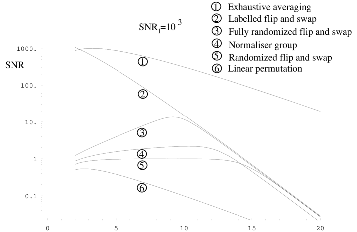
Graphs of the behavior of the signal to noise ratio of this and the other methods are given in Figure 2. For small $n$, the limited number of possible random choices results in a significant reduction in the signal to noise ratio. However, a reasonable number of repetitions of the experiment can still reliably determine any bias in $x$, if $x$ is not too small. An improvement in the SNR can also be obtained by using randomization over the normalizer group as discussed in Section V. This is called fully randomized flip&swap.

FIG. 2.: Graphs of lower bounds on the signal to noise ratio for the different averaging methods for two or more identical non-interacting qubits at high temperature, and $|x|=1$. The bounds hold for a one qubit signal to noise ratio of $10^{3}$. The signal to noise ratios are for one experiment in the case of randomization over a group, two in the case of flip&swap and $2^{n}-1$ in the case of exhaustive averaging. The noise is due both to experimental sensitivity and contributions from randomization (except for labeled flip&swap and exhaustive averaging, which involve no randomization). Repeating the experiments $k$ times with independent random choices increases the signal to noise ratios by a factor of $k^{1/2}$.

Labeled flip&swap requires $n+1$ qubits and applies the flip&swap operation to all them. Instead of removing the polarization in ${|\mbox{\bf 1}\rangle}$ by averaging, it is exploited by using the $n+1$’th qubit as a label similar to the methods introduced in [2]. This method was discovered independently by D. Leung. Conditionally on the $n+1$’th qubit being in state ${|0\rangle}$, the first $n$ qubits are in an effective pure state with excess probability in ${|\mbox{\bf 0}\rangle}$. Conditionally on the $n+1$’th qubit being in state ${|1\rangle}$, the first $n$ qubits are in an effective pure state, but with a deficiency in ${|\mbox{\bf 1}\rangle}$. Both experiments’ preparation steps must be followed by an operation which conditionally on the $n+1$’th qubit flips all the other qubits to turn the conditional deficiency in ${|\mbox{\bf 1}\rangle}$ into one in ${|\mbox{\bf 0}\rangle}$. After the computation is complete, the deficiency can be turned into an effective excess by conditionally reversing the sign of the answer. The full network for $n=3$ is given in Figure 3.

FIG. 3.: Quantum networks for the two experiments to implement labeled flip&swap for three computational qubits. The readout operation on qubit A is shown explicitly as a triangle. Filled circles denote conditioning on $|1>$, while unfilled circles denote conditioning on $|0>$.

The signal to noise ratio for labeled flip&swap is given by

SNR $$= {\sqrt{2}(n+1)|x|\mbox{SNR}_{1}\over 2^{n}}.$$ (63)

V Randomization over Groups

Exhaustive averaging is useful for small numbers of qubits and flip&swap works for nearly non-interacting qubits at high temperatures. If the number of qubits and the polarization satisfy $n\delta\sim 1$ or if the initial state does not have approximate inversion symmetry, it is necessary to consider other methods which are both reasonably efficient and can be applied to arbitrary initial states. Randomization based on groups of unitary operators has this property.

In general, randomization involves choosing a preparation operator $P$ according to a predetermined probability distribution. To ensure that the expected value of the measurement represents the output of the computation on an effective pure state, we require that $\mbox{Exp}_{P}(P\rho P^{\dagger})=\bar{\rho}$ is an effective pure state. The methods to be discussed satisfy that

$$\bar{\rho} = (\rho_{00}-\bar{p}){|0\rangle}{\langle 0|}+\bar{p}I,$$ (64)

with $\bar{p}={1\over N-1}\sum_{i\geq 1}\rho_{ii}$. It is desirable that the initial state $\rho$ has excess probability in the ground state. If possible, the true initial state should be transformed by a unitary transformation which guarantees that the maximum probability state is the ground state, and that the density matrix is diagonal in the computational basis. (For nearly uniform mixtures of states and high sensitivity, it may be more efficient to have a sufficiently large deficiency in the ground state.)

Let $\sigma=C^{\dagger}\sigma_{z}^{(1)}C$, so that $x=\mbox{tr}({|0\rangle}{\langle 0|}\sigma)=\sigma_{00}$. A single experiment with randomized preparation yields the measurement $r(P)=\mbox{tr}(P\rho P^{\dagger}\sigma)$ with variance $s^{2}$; the expectation of $r(P)$ is given by $\bar{r}=(\rho_{00}-\bar{p})x$. The signal to noise ratio for a single run of the computation is determined by comparing the variance $\bar{v}$ of $r(P)$ to $\bar{r}^{2}$. Thus, the signal to noise ratio is

$$\mbox{SNR}(P,C,\rho)={|\bar{r}|\over\sqrt{s^{2}+\bar{v}}}.$$ (65)

If, for example, we wish to learn the expectation of $\bar{r}$ to within $\bar{r}(1\pm\epsilon)$, the number of experiments required to achieve confidence $c$ is proportional to $\log(1/c)/(\epsilon^{2}\mbox{SNR}(P,C,\rho)^{2})$ in the Gaussian regime. Due to the large number of choices in the randomization it is reasonable to expect that this regime applies even for one experiment. If this is were not the case, the average would need to be inferred by techniques robust against outliers. If we are only interested in learning the sign of $\bar{r}$ with confidence $c$, this can be done with $\sim\log(1/c)/\mbox{SNR}(P,C,\rho)^{2}$ experiments, regardless of the actual distribution. One method is to use the sign of the median of the $k_{1}$ averages of the results from $k_{2}\doteq\max(1,4/\mbox{SNR}(P,C\rho)^{2})$ independent experiments. Because the probability of the event that the average of $k_{2}$ experiments has the wrong sign is bounded by $1/4$, the probability of failure is $\leq e^{-O(k_{1})}$. The constant in the exponent can be obtained from the Chernoff-Hoeffding bounds [10] for the probablity of having more than $1/2$ heads in $k_{1}$ flips of a biased coin with the probability of head given by $1/4$.

To compute the variance of $r(P)$, define

$$\check{\rho} \doteq \rho-\mbox{Exp}_{P}P\rho P^{\dagger}$$ (66)

$$= \rho-\bar{p}I-(\rho_{00}-\bar{p}){|0\rangle}{\langle 0|}.$$ (67)

Then

$$\bar{v} = \mbox{Exp}_{P}\mbox{tr}(P\check{\rho}P^{\dagger}\sigma)^{2}$$ (68)

$$= \mbox{Exp}_{P}\mbox{tr}((P\check{\rho}P^{\dagger}\otimes P\check{\rho}P^{\dagger})(\sigma\otimes\sigma))$$ (69)

$$= \mbox{tr}(\mbox{Exp}_{P}(P\check{\rho}P^{\dagger}\otimes P\check{\rho}P^{\dagger})(\sigma\otimes\sigma)).$$ (70)

Thus to ensure that $\bar{r}$ is as desired and to compute $\bar{v}$, we first verify that $\mbox{Exp}_{P}(P\check{\rho}P^{\dagger})=0$ and then compute $\mbox{Exp}_{P}(P\check{\rho}P^{\dagger}\otimes P\check{\rho}P^{\dagger})$.

In the algorithms described below, $P$ is a random product of operators, each chosen uniformly from various groups of unitary operators. The desired expectations can often be computed in closed form if $P$ is a random element of a unitary group $G$. For this purpose, it is convenient to use the representations of $G$ defined by $\pi_{1}(P)(A)=PAP^{\dagger}$ and $\pi_{2}(P)(A\otimes B)=PAP^{\dagger}\otimes PBP^{\dagger}$, where $\pi_{2}(P)$ is linearly extended to all four-tensors. Both $\pi_{1}$ and $\pi_{2}$ are unitary representations of $G$ for the usual inner product of operators and four-tensors: $\langle A,B\rangle=\mbox{tr}(AB)$ and $\langle A\otimes B,C\otimes D\rangle=\mbox{tr}(AC)\mbox{tr}(CD)$, with the latter inner product extended bilinearly to all four-tensors. Using this representation, for $P$ sampled uniformly from $G$, it follows that the expectations can be obtained by projecting $\rho$ and $\rho\otimes\rho$ onto the trivial eigenspaces of $\pi_{1}$ and $\pi_{2}$. Specifically, let $\Pi_{1}$ and $\Pi_{2}$ be the projection superoperators onto the space of all $A$ such that $\pi_{1}(P)A=A$ and onto the space of all $B$ such that $\pi_{2}(P)B=B$, respectively. Then $\mbox{Exp}_{P\in G}\pi_{1}(P)A^{\dagger}=\Pi_{1}A$ and $\mbox{Exp}_{P\in G}\pi_{2}(P)B=\Pi_{2}B$. We use this to calculate variances resulting from averaging over four groups, below.

A Diagonal Groups

If the initial density matrix is not diagonal and it is not feasible to perform the unitary transformation which makes it diagonal in the computational basis, one can use randomization over a diagonal group to reduce the effect of the offdiagonal entries. Let ${\cal D}$ be a group of diagonal operators $S_{f}:{|j\rangle}\rightarrow i^{f(j)}{|j\rangle}$, with $f(j)\in\{0,1,2,3\}$. To ensure sufficiently small trivial eigenspaces for the representations $\pi_{1}$ and $\pi_{2}$, we require that the following phase independence condition holds: If $f(j)-f(k)+f(l)-f(m)=0\;\mbox{mod}(4)$ for all $f$, then $j=k$ and $l=m$ or $j=m$ and $k=l$. We call a group with this property a diagonal group. Randomization over ${\cal D}$ is accomplished by choosing a member of ${\cal D}$ uniformly and applying it to the initial state. Although the expectation of the randomized density matrix is not yet an effective pure state, it does reduce the off-diagonal contributions to the expectation and the variance. For example,

$$\mbox{Exp}_{P\in{\cal D}}P\rho P^{\dagger} = \sum_{i=0}^{N-1}\rho_{ii}{|i\rangle}{\langle i|}.$$ (71)

To obtain an effective pure state, additional randomization steps are required. The expectations needed for computing variances are calculated in the appendix. An efficiently implementable diagonal group ${\cal D}$ can be obtained as a subgroup of the normalizer group introduced below.

B Two-transitive Permutation Groups

Let ${\cal T}$ be a two-transitive group of permutations acting on the set of states ${|1\rangle},\ldots,{|N-1\rangle}$. By definition, for every $i\not=j$ and $k\not=l$, there is a permutation $\pi\in{\cal T}$ such that $\pi(i)=k$ and $\pi(j)=l$. Then

$$\mbox{Exp}_{P_{1}\in{\cal D},P_{2}\in{\cal T}}P_{2}P_{1}\rho P_{1}^{\dagger}P_{2}^{\dagger} = (\rho_{00}-\bar{p}){|0\rangle}{\langle 0|}+\bar{p}I,$$ (72)

which is the desired effective pure state. An effective pure state would be obtained on average even with a one-transitive group, such as the cyclic permutations used for exhaustive averaging. However, the variance for one-transitive groups can be quite large and two-transitivity helps in reducing it.

To give the upper bound on $\bar{v}$ for randomization with ${\cal D}$ and ${\cal T}$, define

$$\check{\rho}_{d} \doteq \sum_{i\geq 1}\check{\rho}_{ii}{|i\rangle}{\langle i|},$$ (73)

Then

$$\bar{v} \leq \mbox{tr}(\check{\rho}_{d}^{2})+{1\over N-2}\mbox{tr}(\check{\rho}^{2}).$$ (74)

The derivation of this inequality is in the appendix. In the high temperature regime, this implies a signal to noise ratio of at least

SNR $$\geq {n\over 2^{n}}{|x|\mbox{SNR}_{1}\over\sqrt{1+n\mbox{SNR}_{1}^{2}/(2^{n}-2)}}.$$ (75)

Efficiently implementable two-transitive permutation groups can be obtained from the normalizer group.

C The Normalizer Group

The normalizer group ${\cal N}$, more specifically, the normalizer of the error group, consists of all unitary operations $U$ which satisfy that for any tensor product of Pauli operators $\sigma$, $U\sigma U^{\dagger}$ is also a tensor product of Pauli operators (up to a phase factor). If the Pauli operators are labeled by $\sigma_{00}\doteq I,\sigma_{01}\doteq\sigma_{z},\sigma_{10}\doteq\sigma_{x},\sigma_{11}\doteq\sigma_{y}$ and, for example, $\sigma_{101101}=\sigma_{10}\otimes\sigma_{11}\otimes\sigma_{01}$, then the elements of the normalizer group are characterized by $U\sigma_{b}U^{\dagger}=(-1)^{\langle x,b\rangle}i^{f(b,L)}\sigma_{Lb}$, where $x$ is an arbitrary bit vector, $\langle x,b\rangle$ denotes the inner product modulo $2$ of bit vectors and $L$ is an arbitrary invertible (modulo 2) 0-1 matrix which satisfies $L^{T}ML=M$, where $Mb$ is the bit vector obtained from $b$ by swapping adjacent bits belonging to the same factor. The exponent $f(b,L)$ depends only on $b$ and $L$; its values are not needed for the present analyses. The group of matrices $L$ with this property acts transitively on non-zero bit vectors. The normalizer group yields several subgroups useful for randomization.

Linear Phase Shifts.

The group ${\cal D}$ generated by controlled-sign flips and the operator $S=\scriptstyle\left(\begin{array}[]{cc}1&0\\ 0&i\end{array}\right)$ acting on any qubit consists of diagonal operators with action ${|k\rangle}\rightarrow i^{\langle x,k\rangle}(-1)^{\langle k,Bk\rangle}{|k\rangle}$, where $x$ is a vector with entries in $\{0,1,2,3\}$ and $B$ is an arbitrary $n$ by $n$ 0-1 matrix. To check that the phase independence condition (Section V A) holds, suppose that for all $x$ and $B=yz^{T}$,

$$x^{T}(k-l+m-n)+2(k^{T}yz^{T}k-l^{T}yz^{T}l+m^{T}yz^{T}m-n^{T}yz^{T}n) = 0\;\mbox{mod}(4).$$ (76)

This implies that $k-l+m-n=0\;\mbox{mod}(4)$. If $k=m$, then $l=n=k$, since $k,l,m$ and $n$ are all 0-1 vectors. If not, without loss of generality, suppose that $k\not=0$. To derive a contradiction, suppose also that $k\not=l$ and $k\not=n$. If $k$ is not in the span (modulo two) of $l,m$ and $n$, then there exists $z$ orthogonal (modulo two) to $l,m$ and $n$, but not $k$, which contradicts the equality above. Thus $k$ must be in the span of $l,m$ and $n$. If $k$ is not in the span of two of them, say $l$ and $m$, then there exists $z$ orthogonal to $l$ and $m$ but not $k$ and a $y$ orthogonal to $n$ but not $k$. Again, we find that the equality cannot hold. Thus it must be the case that $k=l+m\;\mbox{mod}(2)$, $k=l+n\;\mbox{mod}(2)$ and $k=m+n\;\mbox{mod}2$. This implies that $m=n=l$ and $k=0$. Thus the desired independence condition holds.

Linear Cyclic Permutations.

A group ${\cal S}$ acting cyclicly on the set ${|1\rangle},\ldots,{|n\rangle}$ is obtained by representing the field $\mbox{GF}(2^{n})$ as a vector space over $\mbox{GF}(2)$ with elements represented by bit strings of length $n$ in some basis. Multiplication by non-zero elements of $\mbox{GF}(2^{n})$ defines a cyclic subgroup of ${\cal L}$ of order $2^{n}-1$.

Linear Permutations.

The group ${\cal T}$ of linear permutations is generated by the controlled-not operations. The group consists of the unitary $U$’s which satisfy $U{|b\rangle}={|Lb\rangle}$, where $L$ is an invertible (modulo two) 0-1 matrix. The group acts two-transitively on the set ${|1\rangle},\ldots,{|N\rangle}$.

D Conditional Normalizer Group

Randomization over the normalizer group is as effective for variance reduction as is randomization over the unitary group. The main difficulty is that the normalizer group does not fix ${|0\rangle}$. This can be remedied by alternating randomization with ${\cal T}$ and with the conditional normalizer group ${\cal N}_{1}$ which acts on the first $n-1$ qubits given that the last one is in state ${|1\rangle}$.

The first step in the procedure is to randomize with ${\cal D}$ (if needed) and ${\cal T}$. Each following step involves randomizing with ${\cal N}_{1}$ and then with ${\cal T}$. The total number of steps determines how effective the randomization is. The procedure is designed such that the expectation of the resulting density matrix is the desired effective pure state after every step. The variance $\bar{v}_{k+1}$ after the $k$’th step can be estimated by (see the appendix):

$$\bar{v}_{k+1} \leq \lambda^{k}{N\over N-2}\mbox{tr}(\check{\rho}_{d}^{2})+{1\over N-2}\check{\rho}^{2},$$ (78)

with $\lambda\doteq{e^{1\over N+2}/2}$. In the high temperature regime this implies a signal to noise ratio of

SNR $$\geq {n\over 2^{n}}{|x|\mbox{SNR}_{1}\over\sqrt{1+2n\mbox{SNR}_{1}^{2}/(2^{n}(2^{n}-1))}},$$ (79)

where $k$ was chosen such that $\lambda^{k}\leq{1/2(2^{n}+2)}$.

VI Effective Pure States by Entanglement

The temporal randomization methods discussed above are useful when the device is qubit limited, in the sense that it is difficult to access additional qubits. It is important to realize that ancillary qubits involved only in preparation and postprocessing generally do not need to have long decoherence or relaxation times. For example, if they are used only in the preparation phase, their quantum coherence does not need to be maintained in computation or readout. If such ancillas are available, they can and should be used to simplify the effective pure state preparation. Interestingly, if an additional $n$ qubits are available, it is possible to prepare a nearly perfect effective pure state for any diagonal initial state by exploiting entanglement.

Here is an explicit algorithm which results in an effective pure state on the first $n$ qubits given $2n$ qubits. The basic idea is to map the computational basis states other than the ground state on the first $n$ qubits to nearly maximally entangled states. Write a computational basis state on the $2n$ qubits as ${|a\rangle}{|b\rangle}$, where $a$ and $b$ are length $n$ bit vectors. Let $x$ be a generator of the multiplicative group of non-zero elements of $\mbox{GF}(2^{n})$. The desired unitary transformation is the composition of the maps

$$P_{1} : {|a\rangle}{|b\rangle}\rightarrow\sum_{c}(-1)^{\langle b,c\rangle}{|a\rangle}{|c\rangle},$$ (80)

$$P_{2} : {|a\rangle}{|b\rangle}\rightarrow{|ax^{b}\rangle}{|b\rangle},$$ (81)

where $b$ is interpreted as a bit vector in the first exponent and as a binary number in the second. Consider the reduced density matrix $\varrho_{ab}$ on the first $n$ qubits derived from the state $P_{2}P_{1}{|a\rangle}{|b\rangle}$. If $a\not=0$,

$$\varrho_{ab} = {1\over N}(I-{|0\rangle}{\langle 0|}+{|a\rangle}{\langle a|})$$ (82)

$$\varrho_{0b} = {|0\rangle}{\langle 0|}.$$ (83)

This is nearly an effective pure state. If $\rho$ is the reduced initial density matrix on the first $n$ qubits and $\rho$ is diagonal, then after applying $P_{2}P_{1}$, the reduced density matrix is

$${N-1\over N}((\rho_{00}-\bar{p}){|0\rangle}{\langle 0|}+\bar{p}I)+{1\over N}\rho.$$ (84)

The deviation from the effective pure state is sufficiently small to be of no concern in most cases.

Entanglement can be exploited even if less than $n$ additional bits are available. In fact, essentially the same algorithm works. However, the deviation from an effective pure state becomes larger and residual bias must be removed by another technique such as randomization. In general, if ancillary qubits are available, the effectiveness of averaging methods can be improved. For example, we can randomize the states ${|a\rangle}{|b\rangle}$ with $a\not=0$ with the subgroup ${\cal L}_{m}$ of the group of linear permutations which preserves the subspace $\{{|0\rangle}{|b\rangle}\}$. If this does not reduce the variance enough, a version of the conditional normalizer randomization method can be used, where ${\cal L}_{m}$ is used instead of the full group of linear permutations.

Ancillary qubits are likely to be available whenever a computational cooling method is used to increase the probability of the ground state in some of the available qubits. Computational cooling uses ancillas and in-place operations to transfer heat from the computational qubits to the ancillas. The simplest such methods are based on decoding a classical error-correcting code in-place and exploiting the fact that the thermal state is equivalent to a noisy ground state.

VII Experimental Evidence

The temporal randomization methods can find immediate application in NMR quantum computation, even with simple molecules, as we demonstrate with the following experimental results utilizing exhaustive averaging to extract an effective pure state from a two spin system.

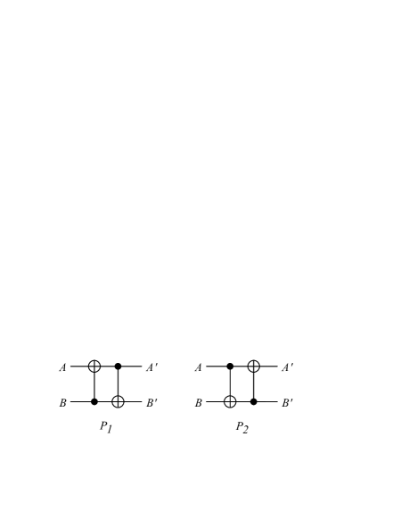
Using a model two spin system, we prepared an effective state similar to that of Eq.(54) from a thermal state. This was done by implementing the quantum circuits shown in Fig. 4 to perform the permutation of Eq.(17) and its inverse.

FIG. 4.: Quantum circuit implementation of the permutations $P_{1}$ and $P_{2}$.

The two-spin physical system used in these experiments was carbon-13 labeled chloroform (Fig. 5) supplied by Cambridge Isotope Laboratories, Inc. (catalog no. CLM-262), and used without further purification. A 200 millimolar sample was prepared with d6-acetone as a solvent, degassed, and flame sealed in a standard 5mm NMR sample tube, at the U.C. Berkeley College of Chemistry.

FIG. 5.: Molecule of chloroform: the two active spins in this system are the ¹³C and the ¹H.

Spectra were taken using Bruker AMX-400 (U.C. Berkeley) and DRX-500 (Los Alamos) spectrometers using standard probes. The resonance frequencies of the two proton lines (in the DRX-500) were measured to be at $500.133921$ MHz and $500.134136$ MHz, and the carbon lines were at $125.767534$ MHz and $125.767749$ MHz, with errors of $\pm 1$ Hz. The radiofrequency (RF) excitation carrier (and probe) frequencies were set at the midpoints of these peaks, so that the chemical shift evolution could be suppressed, leaving only the $215$ Hz J-coupling between the two spins. The $T_{1}$ and $T_{2}$ relaxation times were measured using standard inversion-recovery and Carr-Purcell-Meiboom-Gill pulse sequences. For the proton, it was found that $T_{1}\approx 7$ sec, and $T_{2}\approx 2$ sec, and for carbon, $T_{1}\approx 16$ sec, and $T_{2}\approx 0.2$ sec. The short carbon $T_{2}$ time is due to coupling with the three quadrupolar chlorine nuclei, which shortens the coherence time. Nevertheless, these time scales were all much longer than those of the operations applied, guaranteeing that we could implement quantum transforms and observe quantum dynamics.

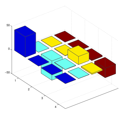
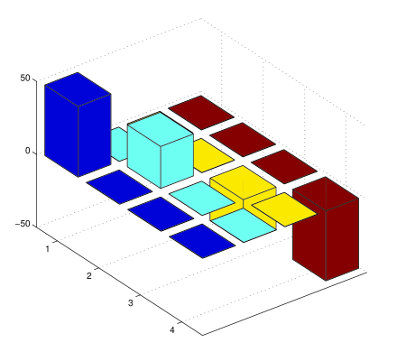
We performed quantum state tomography to systematically obtain the final quantum state; this procedure will be described in detail elsewhere [11]. In each tomography procedure, nine experiments were performed, applying different pulses to measure all the possible elements in the density matrix in a robust manner. The resulting deviation density matrix for the thermal state is shown in Fig. 7A. As expected, all the off-diagonal elements are nearly zero, while the diagonal elements follow a pattern of $a+b$, $a-b$, $-a+b$, and $-a-b$. An error of about $5$% was observed in the data, due primarily to imperfect calibration of the $90^{\circ}$ pulse widths and inhomogeneity of the magnetic field.

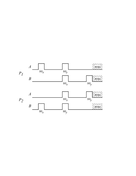
FIG. 6.: NMR pulse program implementations of the permutations $P_{1}$ and $P_{2}$. Each RF pulse was about $10$ microseconds long, and the time between the pulses was about $2.3$ milliseconds.

The two permutation quantum circuits were implemented using the pulse programs shown in Fig. 6. Because of the absence of phase correction steps in the controlled-not gates[2], the actual transforms implemented were not exactly those of Eq.(17), but rather,

$$\tilde{P}_{1} = \left[\begin{array}[]{cccc}i&0&0&0\\ 0&0&-1&0\\ 0&0&0&1\\ 0&i&0&0\end{array}\right]$$ (89)

$$\tilde{P}_{2} = \left[\begin{array}[]{cccc}i&0&0&0\\ 0&0&0&1\\ 0&-1&0&0\\ 0&0&i&0\end{array}\right]\,.$$ (94)

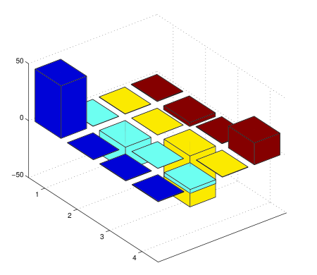
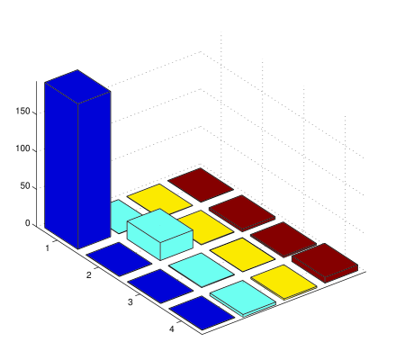
For the purposes of temporal randomization of an initially diagonal density matrix, the phases of the transformations can be ignored. We obtained the density matrices shown in Fig. 7B-C from these two transformations. The effective pure state we obtained was approximately

$$\bar{\rho}=\left[\begin{array}[]{cccc}194&\epsilon&\epsilon&\epsilon\\ \epsilon&24&\epsilon&\epsilon\\ \epsilon&\epsilon&\epsilon&\epsilon\\ \epsilon&\epsilon&\epsilon&8\end{array}\right]-57I\,,$$ (95)

where $|\epsilon|<5.4$. An error of $\pm 5$ was calculated, based on analysis of the linewidth integration, least squares fitting used in the tomography procedure, and standard error propagation. This result compares favorably with the result expected from Eq.(54). Further work has been done to use this state as an input into a non-trivial computation; that work demonstrates the creation and manipulation of effective pure states which are in superpositions, and will be reported elsewhere[11].

(A)     (B) 

(C)     (D) 

FIG. 7.: Experimentally measured deviation density matrices for (A) thermal state, (B) state after $P_{1}$ operation, (C) state after $P_{2}$ operation. (D) Effective pure state (biased sum of the three). Real components only are shown; all imaginary components are small.

VIII Conclusion

We have described new techniques for creating effective pure states which complement the logical labeling and spatial averaging techniques previously discovered. Our temporal averaging methods are unique in their use of summation over experiments carried out at different times and powerful by virtue of averaging over transformations chosen systematically (in the case of labeled flip&swap) or randomly (for randomization over a transformation group). The choice of temporal averaging method in an experiment depends on the number of qubits available, how many are required for computation, the initial density matrix and the desired signal to noise ratio. A summary of our recommendations based on the analyses in this manuscript follows: For small numbers of qubits exhaustive averaging can be used for any initial density matrix which is diagonal in the computational basis. If the initial state is close to that of non-interacting particles at high temperature, the flip&swap techniques can be used. If a non-computational qubit is available, then labeled flip&swap is the simplest and most efficiently implemented method. Asymptotically it requires a linear number of quantum operations, and unless high signal to noise ratios are needed, involves many fewer experiments than exhaustive averaging. In terms of quantum operations, exhaustive averaging appears to be more efficient up to at least four qubits. The actual minimum number of qubits for which labeled flip&swap uses fewer quantum operations per experiment then exhaustive averaging depends on the implementation and remains to be determined. If every qubit is required for computation, then randomized flip&swap can be used at a cost of more quantum operations per experiment. For large numbers of qubits where the high temperature regime or the non-interacting assumption fails, randomization over a group can be used. If ancillary qubits are available, randomization can be combined with entanglement. It remains to be seen whether this situation will be encountered in practice.

Future theoretical work will investigate combinations of logical, spatial, and temporal labeling techniques, and establish a connection between these procedures and error-correction. Experiments will also be performed to demonstrate the different techniques with large molecules and to explore their relative merits in practice.

Acknowledgements. D. Leung independently discovered that labeling and temporal averaging could be combined in the high temperature regime by labeled flip&swap. Thanks to W. Zurek for encouraging our work on NMR quantum computation. We profited from stimulating discussions with J. Anglin and D. Divincenzo, and ackowledge M. Kubinec, P. Catasti and S. Velupillai for experimental assistance. In particular we thank S. Velupillai for suggesting the use of labeled chloroform in the experiment. This work was performed under the auspices of the U.S. Department of Energy under Contract No. W-7405-ENG-36.

A Calculations of Variance for Randomization over Groups

The expectation and variance of the outcome of an experiment using randomization over a group $G$ can be determined from the trivial eigenspaces of the representations $\pi_{1}:\pi_{1}(U)(A)=UAU^{\dagger}$ and $\pi_{2}:\pi_{2}(U)(A\otimes B)=UAU^{\dagger}\otimes UBU^{\dagger}$. In the next sections, these eigenspaces are determined and the resulting variances estimated. We begin with some calculations for the diagonal groups.

1 Diagonal Groups

Let ${\cal D}$ be a diagonal group as defined in Section V A. This group is used to diagonalize the average density matrix before randomizing with more powerful groups. We compute the projections onto the trivial eigenspaces of both representations $\pi_{1}$ and $\pi_{2}$.

$$\mbox{Exp}_{P\in{\cal D}}P{|i\rangle}{\langle j|}P^{\dagger} = \delta_{i,j}{|i\rangle}{\langle i|},$$ (A1)

and

$$\mbox{Exp}_{P\in{\cal D}}P{|i\rangle}{\langle i|}P^{\dagger}\otimes P{|k\rangle}{\langle k|}P^{\dagger} = {|i\rangle}{\langle i|}\otimes{|k\rangle}{\langle k|},$$ (A2)

$$\mbox{Exp}_{P\in{\cal D}}P{|i\rangle}{\langle k|}P^{\dagger}\otimes P{|k\rangle}{\langle i|}P^{\dagger} = {|i\rangle}{\langle k|}\otimes{|k\rangle}{\langle i|}.$$ (A3)

Other expectations of ${|i\rangle}{\langle j|}\otimes{|k\rangle}{\langle l|}$ are $0$. The projections of $\check{\rho}$ and $\check{\rho}\otimes\check{\rho}$ onto the trivial eigenspaces of $\pi_{1}$ and $\pi_{2}$ are therefore given by

$$\mbox{Exp}_{P\in{\cal D}}P\check{\rho}P^{\dagger} = \sum_{i\geq 0}\check{\rho}_{ii}{|i\rangle}{\langle i|},$$ (A4)

$$\mbox{Exp}_{P\in{\cal D}}P\check{\rho}P^{\dagger}\otimes P\check{\rho}P^{\dagger} = \sum_{i,j\geq 0}\check{\rho}_{ii}{|i\rangle}{\langle i|}\otimes\check{\rho}_{jj}{|j\rangle}{\langle j|}+\sum_{i\not=j\geq 0}\check{\rho}_{ij}{|i\rangle}{\langle j|}\otimes\check{\rho}_{ji}{|j\rangle}{\langle i|}.$$ (A5)

Unfortunately, it is impossible to completely eliminate the contributions of the off-diagonal elements of $\rho$ to the variance by this method. As will be seen, to reduce the effect of these contributions it is necessary to ensure that $\rho$ is approximately diagonal by an initial unitary operation, or to design the algorithm so that $\sigma$ is approximately diagonal (as will be the case if the output of the algorithm is deterministic when given one of the computational basis states for input).

The calculations for the other groups to be presented below assume that $\rho$ has already been randomized by a diagonal group. As a result, only the subspaces spanned by ${|i\rangle}{\langle i|}$ (for $\pi_{1}$) and by ${|i\rangle}{\langle i|}\otimes{|j\rangle}{\langle j|}$ (for $\pi_{2}$) and ${|i\rangle}{\langle j|}\otimes{|j\rangle}{\langle i|}$ will be considered in our analysis.

2 Two-transitive Permutation Groups

Let ${\cal T}$ be a two-transitive permutation group which fixes ${|0\rangle}$. It is straightforward to check that for $i\not=j$

$$\mbox{Exp}_{P\in{\cal T}}P{|i\rangle}{\langle i|}P^{\dagger} = {1\over N-1}\sum_{i^{\prime}}{|i^{\prime}\rangle}{\langle i^{\prime}|},$$ (A7)

$$\mbox{Exp}_{P\in{\cal T}}P{|i\rangle}{\langle j|}P^{\dagger} = {1\over(N-1)(N-2)}\sum_{i^{\prime}\not=j^{\prime}}{|i^{\prime}\rangle}{\langle j^{\prime}|},$$ (A8)

where the indices in the sums range from $1$ to $N-1$. This convention for indices and labels will be in place for the remainder of the appendix unless otherwise indicated. The relevant part of the trivial eigenspace of $\pi_{1}$ is spanned by $\check{I}\doteq\sum_{i^{\prime}\geq 1}{|i^{\prime}\rangle}{\langle i^{\prime}|}$ and an operator with no diagonal entries. For $i\not=j$,

$$\mbox{Exp}_{P\in{\cal T}}P{|i\rangle}{\langle i|}P^{\dagger}\otimes P{|i\rangle}{\langle i|}P^{\dagger} = {1\over N-1}\sum_{i^{\prime}}{|i^{\prime}\rangle}{\langle i^{\prime}|}\otimes{|i^{\prime}\rangle}{\langle i^{\prime}|},$$ (A9)

$$\mbox{Exp}_{P\in{\cal T}}P{|i\rangle}{\langle i|}P^{\dagger}\otimes P{|j\rangle}{\langle j|}P^{\dagger} = {1\over(N-1)(N-2)}\sum_{i^{\prime}\not=j^{\prime}}{|i^{\prime}\rangle}{\langle i^{\prime}|}\otimes{|j^{\prime}\rangle}{\langle j^{\prime}|},$$ (A10)

$$\mbox{Exp}_{P\in{\cal T}}P{|i\rangle}{\langle j|}P^{\dagger}\otimes P{|j\rangle}{\langle i|}P^{\dagger} = {1\over(N-1)(N-2)}\sum_{i^{\prime}\not=j^{\prime}}{|i^{\prime}\rangle}{\langle j^{\prime}|}\otimes{|j^{\prime}\rangle}{\langle i^{\prime}|},$$ (A11)

$$\mbox{Exp}_{P\in{\cal T}}P{|0\rangle}{\langle j|}P^{\dagger}\otimes P{|j\rangle}{\langle 0|}P^{\dagger} = {1\over(N-1)}\sum_{j^{\prime}}{|0\rangle}{\langle j^{\prime}|}\otimes{|j^{\prime}\rangle}{\langle 0|},$$ (A12)

$$\mbox{Exp}_{P\in{\cal T}}P{|j\rangle}{\langle 0|}P^{\dagger}\otimes P{|0\rangle}{\langle j|}P^{\dagger} = {1\over(N-1)}\sum_{j^{\prime}}{|j^{\prime}\rangle}{\langle 0|}\otimes{|0\rangle}{\langle j^{\prime}|}$$ (A13)

and expressions involving other combinations of indices which will be of no further concern. The relevant part of the trivial eigenspace of $\pi_{2}$ is therefore spanned (non-orthogonally) by

$$\check{D} \doteq \sum_{i^{\prime}}{|i^{\prime}\rangle}{\langle i^{\prime}|}\otimes{|i^{\prime}\rangle}{\langle i^{\prime}|},$$ (A14)

$$\check{E} \doteq \sum_{i^{\prime},j^{\prime}}{|i^{\prime}\rangle}{\langle i^{\prime}|}\otimes{|j^{\prime}\rangle}{\langle j^{\prime}|},$$ (A15)

$$\check{J} \doteq \sum_{i^{\prime},j^{\prime}}{|i^{\prime}\rangle}{\langle j^{\prime}|}\otimes{|j^{\prime}\rangle}{\langle i^{\prime}|},$$ (A16)

$$\check{Z}_{1} \doteq \sum_{i^{\prime}}{|0\rangle}{\langle i^{\prime}|}\otimes{|i^{\prime}\rangle}{\langle 0|},$$ (A17)

$$\check{Z}_{2} \doteq \sum_{i^{\prime}}{|i^{\prime}\rangle}{\langle 0|}\otimes{|0\rangle}{\langle i^{\prime}|}.$$ (A18)

Define

$$\check{\rho}_{0} \doteq \sum_{i\geq 1}\rho_{0i}{|i\rangle}{\langle 0|}+\rho_{i0}{|0\rangle}{\langle i|},$$ (A19)

$$\check{\rho}_{\bar{0}} \doteq \check{\rho}-\check{\rho}_{0}.$$ (A20)

If $P$ is a random product of operators in ${\cal T}$ and in a diagonal group ${\cal D}$, then

$$\mbox{Exp}_{P_{1}\in D,P_{2}\in{\cal T}}P_{2}P_{1}\check{\rho}P_{1}^{\dagger}P_{2}^{\dagger} = {1\over N-1}\sum_{i}\check{\rho}_{ii}\check{I}=0,$$ (A21)

$$\mbox{Exp}_{P_{1}\in D,P_{2}\in{\cal T}}P_{2}P_{1}\check{\rho}P_{1}^{\dagger}P_{2}^{\dagger}\otimes P_{2}P_{1}\check{\rho}P_{1}^{\dagger}P_{2}^{\dagger} = {1\over N-1}\sum_{i}\check{\rho}_{ii}^{2}\check{D}$$ (A25)

$$\;\;+\;\;{1\over(N-1)(N-2)}\sum_{i\not=j}\check{\rho}_{ii}\check{\rho}_{jj}(\check{E}-\check{D})$$

$$\;\;+\;\;{1\over(N-1)(N-2)}\sum_{i\not=j}\check{\rho}_{ij}\check{\rho}_{ji}(\check{J}-\check{D})$$

$$\;\;+\;\;{1\over N-1}\sum_{i}\check{\rho}_{0i}\check{\rho}_{i0}(\check{Z}_{1}+\check{Z}_{2})$$

$$= {1\over N-1}\mbox{tr}(\check{\rho}_{d}^{2})\check{D}$$ (A29)

$$\;\;+\;\;{1\over(N-1)(N-2)}(\mbox{tr}(\check{\rho}_{\bar{0}})^{2}-\mbox{tr}(\check{\rho}_{d}^{2}))(\check{E}-\check{D})$$

$$\;\;+\;\;{1\over(N-1)(N-2)}(\mbox{tr}(\check{\rho}_{\bar{0}}^{2})-\mbox{tr}(\check{\rho}_{d}^{2}))(\check{J}-\check{D})$$

$$\;\;+\;\;{1\over 2(N-1)}\mbox{tr}(\check{\rho}_{0}^{2})(\check{Z}_{1}+\check{Z}_{2}).$$

The variance $\bar{v}$ is obtained by taking the inner product of this expression with $\sigma\otimes\sigma$. Define

$$\check{\sigma}_{d} \doteq \sum_{i}\sigma_{ii}{|i\rangle}{\langle i|},$$ (A30)

$$\check{\sigma}_{0} \doteq \sum_{i}\sigma_{0i}{|i\rangle}{\langle 0|}+\sigma_{i0}{|0\rangle}{\langle i|},$$ (A31)

$$\check{\sigma}_{\bar{0}} \doteq \sigma-\check{\sigma}_{0}-\sigma_{00}{|0\rangle}{\langle 0|}.$$ (A32)

We will make use of the following (in)equalities:

$$\mbox{tr}\check{\rho} = \mbox{tr}\check{\rho}_{\bar{0}}$$ (A33)

$$= \mbox{tr}\check{\rho}_{d}$$ (A34)

$$= 0,$$ (A35)

$$\mbox{tr}(\rho^{2}) = \mbox{tr}(\check{\rho}_{\bar{0}}^{2})+\mbox{tr}(\check{\rho}_{0}^{2})+\rho_{00}^{2}+(N-1)\bar{p}^{2}$$ (A36)

$$\leq 1,$$ (A37)

$$\mbox{tr}(\check{\sigma}_{\bar{0}}) = -\sigma_{00},$$ (A38)

$$\mbox{tr}(\sigma^{2}) = \mbox{tr}(\check{\sigma}_{\bar{0}}^{2})+\mbox{tr}(\check{\sigma}_{0}^{2})+\sigma_{00}^{2}$$ (A39)

$$= N,$$ (A40)

$$\mbox{tr}(\check{\sigma}_{0}^{2})+2\sigma_{00}^{2} = 2,$$ (A41)

$$\mbox{tr}(\check{\sigma}_{d}^{2}) \leq \mbox{tr}(\check{\sigma}_{\bar{0}}^{2})$$ (A42)

$$\leq N-1,$$ (A43)

where we used the properties of the trace inner product and the fact that $\sigma$ is unitary. The variance can now be estimated by

$$\bar{v} = {1\over N-1}\mbox{tr}(\check{\rho}_{d}^{2})\mbox{tr}(\check{\sigma}_{d}^{2})$$ (A47)

$$\;\;+\;\;{1\over(N-1)(N-2)}(\mbox{tr}(\check{\rho}_{d})^{2}-\mbox{tr}(\check{\rho}_{d}^{2}))(\mbox{tr}(\check{\sigma}_{d})^{2}-\mbox{tr}(\check{\sigma}_{d}^{2}))$$

$$\;\;+\;\;{1\over(N-1)(N-2)}(\mbox{tr}(\check{\rho}_{\bar{0}}^{2})-\mbox{tr}(\check{\rho}_{d}^{2}))(\mbox{tr}(\check{\sigma}_{\bar{0}}^{2})-\mbox{tr}(\check{\sigma}_{d}^{2})))$$

$$\;\;+\;\;{1\over 2(N-1)}\mbox{tr}(\check{\rho}_{0}^{2})\mbox{tr}(\check{\sigma}_{0}^{2})$$

$$\leq \mbox{tr}(\check{\rho}_{d}^{2})+{1\over N-2}\mbox{tr}(\check{\rho}_{d}^{2})+{1\over N-2}(\mbox{tr}(\check{\rho}_{\bar{0}}^{2})-\mbox{tr}(\check{\rho}_{d}^{2}))+{1\over N-1}\mbox{tr}(\check{\rho}_{0}^{2})$$ (A48)

$$\leq \mbox{tr}(\check{\rho}_{d}^{2})+{1\over N-2}\mbox{tr}(\check{\rho}^{2}).$$ (A49)

Both of the terms in this expression can be large compared to $\bar{r}^{2}$. The presence of the second term shows the importance of ensuring that $\rho$ is initially in a nearly diagonal form, and implies a limit on the effectiveness of the diagonal group. However, if $\sigma$ is diagonal in the computational basis, the second term does not arise.

The signal to noise ratio for the thermal distribution can now be obtained as follows. With the definitions from Section IV,

$$\mbox{tr}(\check{\rho}^{2}) = \sum_{i=1}^{N-1}(\rho_{ii}-\bar{p})^{2}$$ (A50)

$$\leq \sum_{i=0}^{N-1}(\rho_{ii}-{1\over N})^{2}$$ (A51)

$$= \sum_{i=0}^{N-1}\rho_{ii}^{2}-{1\over N}$$ (A52)

$$= \prod_{i=1}^{n}{1\over 4}((1+\delta_{i})^{2}+(1-\delta_{i})^{2})-{1\over N}$$ (A53)

$$= {1\over 2^{n}}(\prod_{i=1}^{n}(1+\delta_{i}^{2})-1)$$ (A54)

$$\leq {1\over 2^{n}}(e^{\sum_{i}\delta_{i}^{2}}-1),$$ (A55)

$$\mbox{tr}\check{\rho}^{2} \geq {1\over 2^{n}}\sum_{i}\delta_{i}^{2}.$$ (A56)

The last expression is a good approximation as long as $\sum_{i}\delta_{i}^{2}\ll 1$. The probability of the ground state is given by

$$\rho_{00} = {1\over 2^{n}}\prod_{i=1}(1+\delta_{i})$$ (A57)

$$\geq {1\over 2^{n}}(1+\sum_{i}\delta_{i}),$$ (A58)

which is a good approximation as long as $\sum_{i}\delta_{i}\ll 1$. Thus the signal to noise ratio for randomization using a two-transitive group is bounded by

SNR $$\geq {\sum_{i}\delta_{i}|\sigma_{00}|\over\sqrt{2^{2n}s+2^{n}(1+1/(2^{n}-2))\sum_{i}\delta_{i}^{2}}}.$$ (A59)

To understand the behavior of this expression, consider the case where $\delta_{i}=\delta$ is independent of the qubit. We express $s$ in terms of the signal to noise ratio $\mbox{SNR}_{1}$ for a single qubit, $\mbox{SNR}_{1}\doteq\delta/\sqrt{s}$. For a typical NMR experiment with protons, $\mbox{SNR}_{1}\sim 10^{3}$. With these definitions,

SNR $$\geq {n|\sigma_{00}|\delta\over\sqrt{2^{2n}\delta^{2}/\mbox{SNR}_{1}^{2}+2^{n}(1+1/(2^{n}-2))n\delta^{2}}}$$ (A60)

$$\geq {n\over 2^{n}}{\mbox{SNR}_{1}|\sigma_{00}|\over\sqrt{1+n\mbox{SNR}_{1}^{2}/(2^{n}-2)}}.$$ (A61)

For small $n$, SNR is dominated by the contribution to the variance from the randomization process, while for large $n$, it is dominated by the reduction in excess probability in the ground state.

3 Cyclic Permutation Groups

Consider using a cyclic group ${\cal S}_{1}$ of permutations which leave ${|0\rangle}$ fixed. This was done for exhaustive averaging, but can also be applied to randomization. As we will see, the main problem is that the variance of the measurements cannot be guaranteed to be sufficiently small. Let $\pi$ be a generator of the group of order $N-1$.

The trivial eigenspaces of ${\cal S}_{1}$ can be computed as in the previous section. The relevant subspaces are spanned by $\check{I}$ for $\pi_{1}$ and

$$\check{D}_{k} \doteq \sum_{i\geq 1}{|i\rangle}{\langle i|}\otimes{|\pi^{k}(i)\rangle}{\langle\pi^{k}(i)|},$$ (A62)

$$\check{J}_{k} \doteq \sum_{i\geq 1}{|i\rangle}{\langle\pi^{k}(i)|}\otimes{|\pi^{k}(i)\rangle}{\langle i|},$$ (A63)

$\check{Z}_{1}$, $\check{Z}_{2}$ and a few others of no further concern for $\pi_{2}$.

Let $P$ be a random product of an element of a diagonal group ${\cal D}$ and the cyclic group ${\cal S}_{1}$.

$$\mbox{Exp}_{P_{1}\in{\cal D},P_{2}\in{\cal S}_{1}}P_{2}P_{1}\check{\rho}P_{1}^{\dagger}P_{2}^{\dagger} = 0,$$ (A64)

$$\mbox{Exp}_{P_{1}\in{\cal D},P_{2}\in{\cal S}_{1}}P_{2}P_{1}\check{\rho}P_{1}^{\dagger}P_{2}^{\dagger}\otimes P_{2}P_{1}\check{\rho}P_{1}^{\dagger}P_{2}^{\dagger} = \sum_{k=0}^{N-2}{1\over N-1}\sum_{i}\check{\rho}_{ii}\check{\rho}_{\pi^{k}(i)\pi^{k}(i)}\check{D}_{k}$$ (A67)

$$+\;\;\sum_{k=1}^{N-2}{1\over N-1}\sum_{i}\check{\rho}_{i\pi^{k}(i)}\check{\rho}_{\pi^{k}(i)i}\check{J}_{k}$$

$$+\;\;{1\over 2(N-1)}\mbox{tr}(\check{\rho}_{0}^{2})(\check{Z}_{1}+\check{Z}_{2}).$$

To compute $\bar{v}$ we take the trace after multiplying by $\sigma\otimes\sigma$.

$$\bar{v} = \sum_{k=0}^{N-2}{1\over N-1}\sum_{i}\check{\rho}_{ii}\check{\rho}_{\pi^{k}(i)\pi^{k}(i)}\sum_{i}\sigma_{ii}\sigma_{\pi^{k}(i)\pi^{k}(i)}$$ (A70)

$$+\;\;\sum_{k=1}^{N-2}{1\over N-1}\sum_{i}\check{\rho}_{i\pi^{k}(i)}^{2}\sum_{i}\sigma_{i\pi^{k}(i)}\sigma_{i\pi^{k}(i)}$$

$$+\;\;{1\over N-1}\mbox{tr}(\check{\rho}_{0}^{2})\mbox{tr}(\check{\sigma}_{0}^{2}).$$

The sum involves off-diagonal expressions and products of correlations of the diagonals of $\rho$ and $\sigma$. Although $\bar{v}$ can be much too high in the worst case, in practice one can expect it to be close to what was obtained for a two-transitive group. However, since the known algorithms for the cyclic groups are no more efficient than those for the linear group, there is presently little to be gained by using cyclic groups.

4 The Unitary Group

A spanning set of eigenvectors of the representation $\pi_{2}$ of the unitary group $U$ acting on ${|1\rangle},\ldots,{|N-1\rangle}$ consists of $\check{E}$, $\check{J}$, $\check{Z}_{1}$, $\check{Z}_{2}$ and ${|0\rangle}{\langle 0|}\otimes{|0\rangle}{\langle 0|}$. As a result one obtains

$$\mbox{Exp}_{P\in U}P\check{\rho}P^{\dagger}\otimes P\check{\rho}P^{\dagger} = {1\over 2N(N-1)}((\mbox{tr}\check{\rho}_{d})^{2}+\mbox{tr}(\check{\rho}_{\bar{0}}^{2}))(\check{E}+\check{J})$$ (A73)

$$\;\;+{1\over 2(N-1)(N-2)}((\mbox{tr}\check{\rho}_{d})^{2}-\mbox{tr}(\check{\rho}_{\bar{0}}^{2}))(\check{E}-\check{J})$$

$$\;\;+{1\over 2(N-1)}\mbox{tr}(\check{\rho}_{0}^{2})(\check{Z}_{1}+\check{Z}_{2})$$

$$= {1\over N(N-2)}\mbox{tr}(\check{\rho}_{\bar{0}}^{2})\check{J}-{1\over N(N-1)(N-2)}\mbox{tr}(\check{\rho}_{\bar{0}}^{2})\check{E}+{1\over 2(N-1)}\mbox{tr}(\check{\rho}_{0}^{2})(\check{Z}_{1}+\check{Z}_{2}).$$ (A74)

Thus

$$\bar{v} = {1\over N(N-2)}\mbox{tr}(\check{\rho}_{\bar{0}}^{2})\mbox{tr}(\check{\sigma}_{\bar{0}}^{2})-{1\over N(N-1)(N-2)}\mbox{tr}(\check{\rho}_{\bar{0}}^{2})\mbox{tr}(\check{\sigma}_{d})^{2}+{1\over 2(N-1)}\mbox{tr}(\check{\rho}_{0}^{2})\mbox{tr}(\check{\sigma}_{0}^{2})$$ (A75)

$$\leq {N-1\over N(N-2)}\mbox{tr}(\check{\rho}_{\bar{0}}^{2})+{1\over N-1}\mbox{tr}(\check{\rho}_{0}^{2})$$ (A76)

$$\leq {1\over N-2}\mbox{tr}(\check{\rho}^{2}).$$ (A77)

By using the unitary group, it is possible to eliminate the term $\mbox{tr}\check{\rho}_{d}^{2}$ that occurs in the expression for $\bar{v}$ for the two-transitive permutation groups. Although it is impossible to efficiently implement random elements of the unitary group, there are effective methods for accomplishing the same by using the normalizer group.

5 The Normalizer Group

The normalizer group is as effective at randomizing ${|0\rangle},\ldots,{|N-1\rangle}$ as the full unitary group, at least in terms of expectations and variance. It is straightforward to determine the trivial eigenspaces of $\pi_{1}$ and $\pi_{2}$ in the Pauli operator basis. For $i\not=j$ and $j\not=0$,

$$\mbox{Exp}_{P\in\cal N}P\sigma_{i}P^{\dagger} = \delta_{i,0}\sigma_{0},$$ (A78)

$$\mbox{Exp}_{P\in\cal N}P\sigma_{i}P^{\dagger}\otimes P\sigma_{j}P^{\dagger} = 0,$$ (A79)

$$\mbox{Exp}_{P\in\cal N}P\sigma_{j}P^{\dagger}\otimes P\sigma_{j}P^{\dagger} = {1\over 2^{2m}-1}\sum_{j^{\prime}\not=0}\sigma_{j^{\prime}}\otimes\sigma_{j^{\prime}},$$ (A80)

where $m$ is the number of qubits. Using these identities, it can be verified that the trivial eigenspace of $\pi_{1}$ is spanned by the identity, and that of $\pi_{2}$ by $E\doteq I\otimes I$ and $J\doteq\sum_{i,j\geq 0}{|i\rangle}{\langle j|}\otimes{|j\rangle}{\langle i|}$.

To exploit the normalizer group without removing the polarization in ${|0\rangle}$ requires conditioning it on one of the qubits.

6 Conditional Normalizer Group

In this section we analyze the behavior of the algorithm based on alternate randomizations using ${\cal T}$ and the conditional normalizer group ${\cal N}_{1}$.

Let $\bar{R}_{k-1}$ be the expectation of $P\check{\rho}P^{\dagger}\otimes P\check{\rho}P^{\dagger}$ after the $k$’th step of the conditional normalizer group algorithm. Using Eq.(A29),

$$\bar{R}_{0} = {1\over(N-1)(N-2)}\left(N\mbox{tr}(\check{\rho}_{d}^{2})-\mbox{tr}(\check{\rho}_{\bar{0}}^{2})\right)\check{D}+{1\over(N-1)(N-2)}(\mbox{tr}(\check{\rho}_{\bar{0}}^{2})-\mbox{tr}(\check{\rho}_{d}^{2}))\check{J}$$ (A84)

$$\;\;-\;\;{1\over(N-1)(N-2)}\mbox{tr}(\check{\rho}_{d}^{2})\check{E}$$

$$\;\;+\;\;{1\over 2(N-1)}\mbox{tr}(\check{\rho}_{0}^{2})(\check{Z}_{1}+\check{Z}_{2}).$$

Define $\alpha_{k}$, $\beta_{k}$, $\gamma_{k}$ and $\delta$ by $\bar{R}_{k}\doteq\alpha_{k}\check{D}+\beta_{k}\check{J}+\gamma_{k}\check{E}+\delta(\check{Z}_{1}+\check{Z}_{2})$, where we have used the fact that $(\check{Z}_{1}+\check{Z}_{2})$ are not affected by randomization with ${\cal T}$ and ${\cal N}_{1}$.

Because ${\cal N}_{1}$ distinguishes the state of the first qubit, we need to subdivide the tensors in the expression for $\bar{R}_{0}$. Write $\check{D}=\check{D}_{0}+\check{D}_{1}$, $\check{J}=\check{J}_{00}+\check{J}_{01}+\check{J}_{10}+\check{J}_{11}$ and $\check{E}=\check{E}_{00}+\check{E}_{01}+\check{E}_{10}+\check{E}_{11}$. For example, $\check{D}_{0}=\sum_{i=1}^{N/2-1}{|i\rangle}{\langle i|}\otimes{|i\rangle}{\langle i|}$, $\check{J}_{01}=\sum_{i=1}^{N/2-1}\sum_{j=N/2}^{N-1}{|i\rangle}{\langle j|}\otimes{|j\rangle}{\langle i|}$ and $\check{E}_{10}=\sum_{i=N/2}^{N-1}\sum_{j=1}^{N/2-1}{|i\rangle}{\langle i|}\otimes{|j\rangle}{\langle j|}$, where we are using the convention that the indices $i\geq 2^{n-1}=N/2$ are those referring to states with the first qubit in state ${|1\rangle}$. Randomizing over ${\cal N}_{1}$ preserves all but one of these expressions:

$$\mbox{Exp}_{P\in{\cal N}_{1}}\pi_{2}(P)(\check{D}_{1}) = {2\over N+2}\check{J}_{11}+{2\over N+2}\check{E}_{11}.$$ (A85)

Hence

$$\mbox{Exp}_{P\in{\cal N}_{1}}\pi_{2}(P)(\bar{R}_{k}) = \alpha_{k}\check{D}_{0}+\beta_{k}\check{J}+{2\over N+2}\alpha_{k}\check{J}_{11}+\gamma_{k}\check{E}+{2\over N+2}\alpha_{k}\check{E}_{11}+\delta(\check{Z}_{1}+\check{Z}_{2}).$$ (A87)

Randomizing over ${\cal T}$ gives

$$\mbox{Exp}_{P\in{\cal T}}\pi_{2}(P)(\check{D}_{0}) = {N-2\over 2(N-1)}\check{D},$$ (A88)

$$\mbox{Exp}_{P\in{\cal T}}\pi_{2}(P)(\check{E}_{11}) = {N\over 2(N-1)}\check{D}+{N\over 4(N-1)}(\check{E}-\check{D}),$$ (A89)

$$= {N\over 4(N-1)}\check{D}+{N\over 4(N-1)}\check{E}$$ (A90)

$$\mbox{Exp}_{P\in{\cal T}}\pi_{2}(P)(\check{J}_{11}) = {N\over 2(N-1)}\check{D}+{N\over 4(N-1)}(\check{J}-\check{D})$$ (A91)

$$= {N\over 4(N-1)}\check{D}+{N\over 4(N-1)}\check{J},$$ (A92)

so that

$$\bar{R}_{k+1} = \mbox{Exp}_{P_{2}\in{\cal T}}\mbox{Exp}_{P_{1}\in{\cal N}_{1}}\pi_{2}(P_{2}P_{1})(\bar{R}_{k}))$$ (A93)

$$= \left(1-{N^{2}\over 2(N-1)(N+2)}\right)\alpha_{k}\check{D}+\left(\beta_{k}+{N\over 2(N+2)(N-1)}\alpha_{k}\right)\check{J}+\left(\gamma_{k}+{N\over 2(N+2)(N-1)}\alpha_{k}\right)\check{E}+\delta(\check{Z}_{1}+\check{Z}_{2})).$$ (A94)

The variance $\bar{v}_{k+1}$ after the $k$’th step is given by

$$\bar{v}_{k+1} = \mbox{tr}(\bar{R}_{k+1}\sigma\otimes\sigma)$$ (A95)

$$= \alpha_{k+1}\mbox{tr}(\check{\sigma}_{d}^{2})+\beta_{k+1}\mbox{tr}(\sigma_{\bar{0}}^{2})+\gamma_{k+1}(\mbox{tr}\sigma_{d})^{2}+\delta\mbox{tr}(\sigma_{0}^{2}).$$ (A96)

We can estimate the coefficients as follows:

$$\alpha_{0}\mbox{tr}(\check{\sigma}_{d}^{2}) \leq {N\over N-2}\mbox{tr}(\check{\rho}_{d}^{2}),$$ (A97)

$$\beta_{0}\mbox{tr}(\sigma_{\bar{0}}^{2}) \leq {1\over N-2}(\mbox{tr}(\check{\rho}_{\bar{0}}^{2})-\mbox{tr}(\check{\rho}_{d}^{2})),$$ (A98)

$$\gamma_{0}(\mbox{tr}\check{\sigma}_{d})^{2} = -{1\over(N-1)(N-2)}\mbox{tr}(\check{\rho}_{d}^{2})(\mbox{tr}\check{\sigma}_{d})^{2}$$ (A99)

$$\leq 0,$$ (A100)

$$\delta\mbox{tr}(\check{\sigma}_{0}^{2}) \leq {1\over N-1}\mbox{tr}\check{\rho}_{0}^{2},$$ (A101)

$$\alpha_{k+1}\mbox{tr}(\check{\sigma}_{d}^{2}) = {1\over 2}\left(1+{N-2\over(N-1)(N+2)}\right)\alpha_{k}\mbox{tr}(\check{\sigma}_{d})^{2}$$ (A102)

$$\leq {1\over 2}e^{1\over N+2}\alpha_{k}\mbox{tr}(\check{\sigma}_{d}^{2})$$ (A103)

$$\leq {1\over 2^{k}}e^{k\over N+2}{N\over N-2}\mbox{tr}(\check{\rho}_{d}^{2}).$$ (A104)

Define $\lambda={e^{1\over N+2}/2}$. The coefficients $\beta_{k}$ and $\gamma_{k}$ are monotonically increasing. The limiting values are

$$\beta_{\infty}\mbox{tr}(\check{\sigma}_{\bar{0}}^{2}) = (\beta_{0}+{1\over N}\alpha_{0})\mbox{tr}(\check{\sigma}_{\bar{0}}^{2})$$ (A105)

$$\leq {1\over N-2}\mbox{tr}(\check{\rho}_{\bar{0}}^{2}),$$ (A106)

$$\gamma_{\infty}\mbox{tr}(\check{\sigma}_{d})^{2} = ({1\over N}\alpha_{0}+\gamma_{0})\mbox{tr}(\check{\sigma}_{d})^{2}$$ (A107)

$$\leq 0.$$ (A108)

Thus

$$\bar{v}_{k+1} \leq \lambda^{k}{N\over N-2}\mbox{tr}(\check{\rho}_{d}^{2})+{1\over N-2}\mbox{tr}(\check{\rho}^{2}).$$ (A109)

By choosing $k$ large enough, the variance can be reduced to near that obtainable by randomizing over the whole unitary group. In fact, if $k$ is chosen so that $\lambda^{k}\leq 1/(2(N+2))$, then the maximum contribution to the variance is $\bar{v}\leq{2\over N-1}\mbox{tr}(\check{\rho}^{2})$. Consider the case where $\rho$ is diagonal with $\rho_{00}$ maximal, $c\doteq\sqrt{s}/(\rho_{00}-\bar{p})$ and the output of the algorithm is deterministic (i.e. $\sigma_{00}^{2}=1$). Then ${2\over N-1}\check{\rho}^{2}\leq 2\bar{p}(\rho_{00}-\bar{p})$ and

SNR $$\geq {\rho_{00}-\bar{p}\over\sqrt{s+2\bar{p}(\rho_{00}-\bar{p})}}$$ (A110)

$$\geq {\sqrt{\rho_{00}-\bar{p}}\over\sqrt{c^{2}\rho_{00}+2\bar{p}}}.$$ (A111)

Consequently, if $\bar{p}\ll c\rho_{00}$, the signal to noise ratio is dominated by ${1\over c}$, the term due to measurement noise. If $\bar{p}\gg c\rho_{00}$, then the signal to noise ratio is determined by the contribution from the randomization method. As long as $\bar{p}$ is sufficiently smaller than $\rho_{00}$ and $c\leq 1$ the signal to noise ratio is bounded below by a constant, which ensures that a small number of experiments are required to determine whether $\sigma_{00}=1$ or $\sigma_{00}=-1$. However, in the case where $\bar{p}\sim\rho_{00}$, the signal to noise ratio can be very small, for example if $\rho_{ii}=0$ or $\rho_{ii}=\rho_{00}$ for all $i$. The situation where $\bar{p}\sim\rho_{00}$ is small arises in the high temperature limit of NMR quantum computation. In this case the signal to noise ratio can be estimated as

SNR $$\geq {n\over 2^{n}}{\mbox{SNR}_{1}|\sigma_{00}|\over\sqrt{1+2n\mbox{SNR}_{1}^{2}/(2^{n}(2^{n}-1))}}.$$ (A112)

7 Randomized Flip&Swap

For fully randomized flip&swap, each experimental determination of the output of the computation consists of two experiments. First a sequence of $k$ random operators implementing the conditional normalizer method is chosen. For the present purposes we choose $k$ so that $\lambda^{k}\leq 1/2(N+2)$. Next two experiments are performed. In the first the chosen sequence of operators is applied before measuring $\sigma$. In the second, the flip&swap operation is used before applying the same sequence of random operators and measuring $\sigma$. The measurements are added to obtain the desired answer.

This algorithm behaves exactly like a single randomized experiment with input $\rho_{s}$ (Eq.(61)) and measurement variance $s/2$. The variance of the randomization is therefore given by

$$\bar{v} \leq {2\over N-1}\mbox{tr}(\check{\rho}_{s}^{2})$$ (A113)

$$\leq {2n^{2}\delta^{2}\over N^{2}(N-1)}.$$ (A114)

Substituting in the expression for the signal to noise ratio gives

SNR $$\geq {n\over 2^{n}}{\mbox{SNR}_{1}|\sigma_{00}|\over\sqrt{1/2+2n^{2}\mbox{SNR}_{1}^{2}/2^{2n}(2^{n}-1))}},$$ (A115)

where we have taken into account the fact that two experiments contributed to the signal.

Instead of using the conditional normalizer group, one can use any set of permutation operators $\{P_{i}\}_{i=1}^{N-1}$ with $P_{i}{|0\rangle}={|0\rangle}$ and $P_{i}{|N-1\rangle}={|i\rangle}$. For example, a cyclic linear group can be relabeled to have this property. Because of the symmetries of $\rho_{s}$, this is as effective as using a two-transitive group. Since $\mbox{tr}(\check{\rho}_{s}^{2})\leq n^{2}\delta^{2}/N^{2}$,

$$\bar{v} \leq {(2^{n}-1)n^{2}\delta^{2}\over 2^{2n}(2^{n}-2)}$$ (A116)

and

SNR $$\geq {n\over 2^{n}}{\mbox{SNR}_{1}|\sigma_{00}|\over\sqrt{1/2+n^{2}\mbox{SNR}_{1}^{2}/(2^{n}(2^{n}-2))}}.$$ (A117)

B Implementations of Temporal Averaging Algorithms

1 Flip&Swap

The implementation of labeled flip&swap for three qubits and an ancilla is shown in Figure 3. The flip&swap is the first group of gates, consisting of a not applied to each qubit, followed by controlled-nots from the first to each of the other qubits, an $n-1$-controlled-not conditioned on the last $n-1$ qubits being ${|0\rangle}$, and finally a reversal of the first set of controlled-nots. Efficient quantum networks for the $n-1$-controlled not (generalized Toffoli gates) are given in [12]. Note that for diagonal initial states, phase variants are equivalent, so we can use an SU variant of the Toffoli gate to avoid ancillas while still having an $O(n)$ implementation. Also, the computation can be arranged so that it is $O(n)$ even if controlled operations can only be performed between adjacent qubits in a linear ordering.

An efficient method for implementing randomized flip&swap is to choose for each ${|b\rangle}\not={|\mbox{\bf 0}\rangle}$ an “easy” linear operator $L$ modulo 2 such that $L\mbox{\bf 1}=b$. If $b$ has $w$ one’s, such an operator with at most $n-w$ off-diagonal ones exists. The corresponding unitary operator in the group of linear permutations can be implemented with $n-w$ controlled nots.

2 The Normalizer Group

Every element of the normalizer group ${\cal N}$ operating on $n$ qubits can be implemented by $O(n^{2})$ controlled-nots and $\pi/2$ or $\pi$ rotations of single qubits. For the purposes of randomly choosing one of the members of ${\cal N}$, the natural representation of $U\in{\cal N}$ is

$$U:\sigma_{b}\rightarrow U\sigma_{b}U^{\dagger} = (-1)^{\langle x,b\rangle}i^{f(b,L)}\sigma_{Lb}.$$ (B1)

A uniform random element can be obtained by choosing $x$ and $L$ uniformly subject to $L^{T}ML=M$ (see Section V C). The vector $x$ is obtained by setting each of the $2n$ entries of $x$ independently and uniformly to $0$ or $1$. To obtain uniformly distributed valid $L$’s one can construct $L$ column by column. Write

$$M = \left[\begin{array}[]{cc}0&I\\ I&0\end{array}\right],$$ (B4)

where the entries are $n$ by $n$ matrices and the partitioning is based on writing the index $b$ of $\sigma_{b}$ in the form $b=b_{0}b_{1}$, with $b_{0}$ and $b_{1}$ containing the indices coming from the first and second members of each qubit’s pair, respectively.

If $L_{\leq k}$ is the $2n$ by $k$ matrix consisting of the first $k$ columns of $L$, then $L_{\leq k}^{T}ML_{\leq k}=M_{\leq k,\leq k}$, where $M_{\leq k,\leq k}$ is the $k$ by $k$ matrix submatrix of $M$ in the upper left corner. The columns of $L_{\leq k}$ are linearly independent (modulo $2$). Suppose $L_{\leq k}$ has been constructed and we wish to add another column to obtain $L_{\leq k+1}$. The new column $L_{k+1}$ has to satisfy

$$L_{k+1}^{T}ML_{k+1} = 0,$$ (B5)

$$L_{k+1}^{T}ML_{\leq k} = M_{k+1,\leq k}.$$ (B6)

The first equality is satisfied for any $L_{k+1}$, so we wish to choose $L_{k+1}$ randomly, not in the span of $L_{\leq k}$ and subject to the second equality. The dimension of the affine space of solutions to this equality is $2n-k$, while the dimension of the span of $L_{\leq k}$ is $k$. We consider two cases. If $k<n$, then $M_{k+1,\leq k}=0$, and the span of $L_{\leq k}$ is contained in the space of solutions. Because $2n-k>k$, suitable $L_{k+1}$ can be found. To pick $L_{k+1}$ uniformly one can use any algorithm (e.g. one based on Gaussian elimination modulo $2$) to obtain $2n-2k$ vectors $S_{1},\ldots,S_{2n-2k}$ independent of the columns of $L_{\leq k}$ which together with $L_{\leq k}$ span the solution space. A random $L_{k+1}$ is obtained by choosing a random non-zero linear combination of the $S_{1},\ldots,S_{2n-2k}$ and adding it to a random linear combination of the columns of $L_{\leq k}$.

If $k\geq n$, then $M_{k+1,\leq k}$ is non-zero. If $y$ is in the span of $L_{\leq k}$, then the $k-n+1$’th entry of $y^{T}ML_{\leq k}$ is zero. Since that entry of $M_{k+1,\leq k}$ is $1$, the set of solutions to $y^{T}ML_{\leq k}=M_{k+1,\leq k}$ does not contain any element $y$ in the span of $L_{\leq k}$. We can therefore pick a random element in this affine subspace of dimension $2n-k$. An affine basis for this subspace can again be obtained by a Gaussian elimination method.

The above construction shows that the number of valid $L$’s is $\prod_{k=0}^{n-1}(2^{2n-k}-2^{k})\prod_{k=0}^{n-1}2^{n-k}$. In view of the technique for constructing random invertible matrices over ${\bf Z}_{2}$ given in [13], there are probably more efficient methods for constructing random $L$’s.

To obtain a quantum network which implements the unitary operator defined by $(x,L)$ requires decomposing $L$ into elementary operations corresponding to controlled-nots and single qubit rotations. This can be done by adapting the methods described in [14]. The basic idea is to multiply $L$ on the left and right be the linear operators corresponding to controlled-nots and rotations. Since controlled-nots correspond to elementary row/column operations in the $n$ by $n$ subblocks, one can apply Gaussian elimination methods to convert the first (say) subblock to standard form. The $\pi/2$ rotations around the different axes permit elementary row/column operations between corresponding rows/columns of different subblocks. This can be used to transform $L$ to $I$. The representation of the resulting sequence of controlled-nots and rotations is of the form $(x^{\prime},L)$. To correct the first component, one can apply $\sigma_{M(x-x^{\prime})}$ to the qubits. The total number of gates needed to implement an operator in ${\cal N}$ is $O(n^{2})$ [14].

Implementing ${\cal D}$. Being a subgroup of ${\cal N}$, it is clear that each operator in ${\cal D}$ has an efficient quantum network. The random phase shifts of ${\cal D}$ are described by operators $D(x,B)$ defined by $D(x,B)({|k\rangle})=i^{\langle x,k\rangle}(-1)^{\langle k,Bk\rangle}$. A random such operator is obtained by choosing $x$ randomly and uniformly from all $n$ dimensional vectors over $\{0,1,2,3\}$ and $B$ uniformly from the set of strictly upper triangular $n$ by $n$ $0-1$ matrices. Given such an $x$ and $B$, the phase shifts are implemented by first applying phase shifts by $i^{x_{j}}$ of ${|1\rangle}$ to the $j$’th qubit, and then performing a sequence of controlled-sign flips. The sequence of controlled-sign flips can be read off the entries of $B$ by the following procedure: If $B_{ij}=1$, apply a controlled sign-flip between bits $i$ and $j$. The number of operations required to apply the random phase shift is at most $n(n-1)/2$.

Implementing ${\cal T}$. A unitary operator $U$ in ${\cal T}$ is defined by $U{|b\rangle}={|Lb\rangle}$ for an invertible (modulo $2$) $n$ by $n$ matrix $L$. Any such unitary operator can be implemented using only controlled-nots. Since a controlled not corresponds to an elementary row/column operation, a decomposition of $L$ into such operations yields the desired quantum network. The decomposition can be accomplished by the usual Gaussian elimination methods. A random invertible $L$ can be generated column by column using a simpler version of the method described for the normalizer group. A more efficient algorithm which can be used to construct the decomposition into elementary operations at the same time is described in [13].

3 Entanglement

The operations $P_{1}$ and $P_{2}$ required to implement the method for effective pure states by entanglement are implemented as follows. A phase variant equivalent to $P_{1}$ for diagonal initial states is obtained by applying a $\pi/2$ rotation around the $y$ axis to each of the second group of $n$ qubits. The operation $P_{2}$ is decomposed into the product of $P_{2,i}{|a\rangle}{|b\rangle}\rightarrow{|ax^{b_{i}2^{i}}\rangle}{|b\rangle}$ for $i=0,\ldots,n-1$. Multiplication by $x^{b_{i}2^{i}}$ in $\mbox{GF}(2^{n})$ is a linear map modulo two and defines an element of ${\cal T}$ which can be implemented with $O(n^{2})$ controlled-nots. Each $P_{2,i}$ can therefore be implemented with $O(n^{2})$ Toffoli gates, and $P_{2}P_{1}$ takes $O(n^{3})$ operations.

REFERENCES

• [1] N. Gershenfeld, I. Chuang, and S. Lloyd, in Proceedings of the 4th Workshop on Physics and Computation (New England Complex Systems Institute, Boston, Massachusetts, 1996), p. 134.
• [2] N. A. Gershenfeld and I. L. Chuang, Science 275, 350 (1997).
• [3] D. G. Cory, A. F. Fahmy, and T. F. Havel, in Proceedings of the 4th Workshop on Physics and Computation (New England Complex Systems Institute, Boston, Massachusetts, 1996), pp. 87–91.
• [4] D. G. Cory, A. F. Fahmy, and T. F. Havel, Proceedings of the National Academy of Sciences of the United States of America 94, 1634 (1997).
• [5] B. Schumacher, quant-ph/9604023 (unpublished).
• [6] A. Ekert and R. Jozsa, Reviews of Modern Physics (1993).
• [7] A. Yao, in Proceedings of the 34th Annual Symposium on Foundations of Computer Science (IEEE Press, ADDRESS, 1993), pp. 352–360.
• [8] A. Barenco, Contemporary Physics 37, 375 (1996).
• [9] R. R. Ernst, G. Bodenhausen, and A. Wokaun, Principles of Nuclear Magnetic Resonance in One and Two Dimensions (Oxford University Press, Oxford, 1994).
• [10] N. Alon, J. Spencer, and P. E. os, The Probabilistic Method (John Wiley & Sons, New York, 1992).
• [11] I. L. Chuang, N. Gershenfeld, M. Kubinec, and D. Leung, submitted to Proc. Royal Soc. Lon. A. (unpublished).
• [12] A. Barenco et al., Phys. Rev. A 52, 3457 (1995).
• [13] D. Randall, Random Structures and Algorithms 4, 111 (1993).
• [14] R. Cleve and D. Gottesman, quant-ph/9607030 (unpublished).