Quantum Superposition States of Bose-Einstein condensates

Abstract

We propose a scheme to create a macroscopic “Schödinger cat” state formed by two interacting Bose condensates. In analogy with quantum optics, where the control and engineering of quantum states can be maintained to a large extend, we consider the present scheme to be an example of quantum atom optics at work.

I Introduction

The recent experimental realization of Bose-Einstein condensation of trapped cold rubidium [1], sodium [2], and lithium [3] atoms has initiated new areas of atomic, molecular and optical physics [4]. While some of these new areas remain still somewhat speculative, others have already attained firm experimental grounds, and many of them are based on the analogy between the matter waves and electromagnetic waves, or between bosonic atoms and photons.

On the level of single atoms, the analogy between the matter and electromagnetic waves has led to rapid developments of atom optics [5]. Some authors have thus considered a possibility of nonlinear atom optics in systems of many cold atoms, where the quantum statistical properties and atom-atom interactions become important [6]. It has been also pointed out [7] that nonlinear excitations of Bose-Einstein condensates (BEC) may lead to various analogs of nonlinear optics. Most of these theories have a mean field character, i.e. they disregard quantum fluctuations of the atomic field operators and concentrate on the nonlinear Schödinger-like wave equations for the matter wave functions.

In many situations, such as for example laser cooling or optical imaging, cold atoms not only exhibit their quantum statistical properties, but on top of that they interact with photons. This fact motivated the developments of quantum field theory of atoms and photons [8]. Although this theory accounts in principle for quantum fluctuations of both atomic and electromagnetic fields, the attention has so far been focused predominantly on the latter.

The atom-photon analogy has also triggered the studies in the area of physics of atom lasers [9]. An atom laser, or a boser is a matter wave analog of an ordinary laser. Quite recently, the possibility of employing BEC as a source of coherent matter waves has been demonstrated in the remarkable experiments of the MIT group [10].

We propose here to proceed with this analogy and to look for the implementation of further elements of quantum optics in quantum atom optics. In our opinion, one of the major domains of concern of modern quantum optics is preparation, engineering, control and detection of quantum states in various systems that involve light-matter interactions [11]. By analogy, quantum atom optics, in the sense proposed, concerns preparation, engineering, control and detection of quantum states in atomic systems. Recent studies of excitations in trapped BEC belong to this category, although so far rather limited kinds of time dependent perturbations of the trapping potential [12] were used and only few types of excitation have been investigated. Walsworth and You have proposed a method of selective creation of quasi-particle excitations in trapped BEC [13]. Their method, referred to as spatial magnetic resonance method, could in principle allow for engineering and control of arbitrary excitation in the Bose condensed system.

One of the most spectacular achievements of quantum optics in the recent years has been the observation and study of macroscopic (or strictly speaking mesoscopic) “Schrödinger cat” states of a trapped ion [14], and of an electromagnetic field in a high Q cavity [15]. Schödinger [16] has introduced his famous “cat” states in order to illustrate the fundamental problem of the correspondence between the micro– and macro–worlds: the fact that quantum superposition states are never observed on the macro level. As postulated by von Neumann [17], this is due to irreversible reduction of superposition states into statistical mixtures. Such reduction occurs in any quantum measurement process and leaves the considered system in a mixed state in a “preferred” basis, determined by the measurement. Modern quantum measurement theory [18] describes the reduction process in terms of quantum decoherence due to interactions of the system with environment [19]. Experimental realization of “cat” states requires thus typically sophisticated means to avoid the decoherence effects [14, 15].

In this paper we demonstrate that it is feasible to prepare, control and detect a “Schrödinger cat” formed by two interacting Bose condensates of atoms in different internal states. Atom-atom interactions in our model are mediated through atom-atom collisions and a Josephson-like laser coupling that interchanges internal atomic states in a coherent manner. The theory of such bi-condensates restricted to collisional interactions only has been recently discussed in the Thomas-Fermi approximation [20], and beyond [21, 22]. Amazingly, the simultaneous condensation of ⁸⁷Rb atoms in two internal states (F=2,M=2) and (F=1,M=-1) has been recently achieved at JILA [23], using a combination of evaporative [24] and sympathetic [25] cooling. As pointed out by Julienne et al. [26], the simultaneous condensation was possible due to a very fortunate ratio of elastic/inelastic collision rates for Rb atoms. For the moment, the perspectives of extending the result of [23] to other atomic species are not promising. Nevertheless, one could expect that various ways of modifying atomic scattering lengths will be realized [27], which will allow to control atomic collision processes in a desired way. The above comments apply to the case of magnetic traps. Once it becomes possible to achieve Bose–Einstein condenstaion in, for example, far–off resonance traps, this will open other possibilities of trapping particles with different internal levels. This will allow one to meet in real atomic systems the conditions discussed below for the preparation of Schrödinger cat states.

The plan of the paper is the following. In section II we present the quantum field theoretical model of two trapped condensates, and its simplified two-mode caricature. The detailed analysis of the two-mode model is carried out in section III. We show that in some circumstances the ground state of the system becomes a “Schrödinger cat”, and that the system can be prepared in such a state by adiabatically changing the strength of the Josephson-like laser coupling. Various approximate solutions are tested here in comparison with the exact numerical solution of the problem. In section IV approximate solutions of the complete quantum field theoretical model are found. They display the same qualitative behavior as the one obtained for the two mode model. Finally, in section V we discuss the feasibility of experimental observation of “Schrödinger cat” states of two interacting Bose condensates.

II Quantum field theory of two interacting condensates

We consider here Bose–Einstein condensation of a trapped gas of atoms with two internal levels $|A\rangle$ and $|B\rangle$. The atoms interact via $AA$, $BB$, and $AB$ elastic collisions. Additionally, a set of laser fields drives coherently a Raman transition connecting $|A\rangle\leftrightarrow|B\rangle$. In the formalism of second quantization, such a system is described by the following Hamiltonian

$$H=H_{A}+H_{B}+H_{\rm Int}+H_{\rm Las}$$ (1)

where

$$H_{A,B} = \int d^{3}\vec{x}\;\hat{\Psi}_{A,B}(\vec{x})^{\dagger}\left[-\frac{\hbar^{2}}{2M}\nabla^{2}+\frac{1}{2}M\omega_{A,B}^{2}x^{2}+\frac{4\pi\hbar^{2}a^{\rm sc}_{A,B}}{2M}\hat{\Psi}_{A,B}(\vec{x})^{\dagger}\hat{\Psi}_{A,B}(\vec{x})\right]\hat{\Psi}_{A,B}(\vec{x}),$$ (3)

$$H_{\rm Int} = \frac{4\pi\hbar^{2}a^{\rm sc}_{AB}}{M}\int d^{3}\vec{x}\;\hat{\Psi}_{A}(\vec{x})^{\dagger}\hat{\Psi}_{B}(\vec{x})^{\dagger}\hat{\Psi}_{B}(\vec{x})\hat{\Psi}_{A}(\vec{x})$$ (4)

$$H_{\rm Las} = -\frac{\hbar\Omega}{2}\int d^{3}\vec{x}\left[\hat{\Psi}_{B}(\vec{x})^{\dagger}\hat{\Psi}_{A}(\vec{x})e^{-i\Delta t}+\hat{\Psi}_{A}(\vec{x})^{\dagger}\hat{\Psi}_{B}(\vec{x})e^{+i\Delta t}\right].$$ (5)

Here, $H_{A,B}$ describes the evolution of atoms in $|A\rangle$ and $|B\rangle$, respectively, in the absence of interactions between atoms in different internal states; $H_{\rm Int}$ describes the interactions between atoms in $|A\rangle$ and $|B\rangle$ due to collisions; $H_{\rm Las}$ describes the Raman transitions induced by the laser detuned by $\Delta$ from the Raman resonance; such interactions act as a Josephson-like coupling which transfers coherently particles between $|A\rangle$ and $|B\rangle$, at a Rabi frequency $\Omega>0$. Atoms are confined in harmonic potentials of frequencies $\omega_{A,B}$, and $a^{\rm sc}_{A,B,AB}$ are the scattering lengths for the corresponding collisions, respectively. We assume that the collisions are purely elastic, and that they do not change the number of particles in each internal level.

The field operators $\hat{\Psi}_{A,B}(\vec{x})$, $\hat{\Psi}_{A,B}(\vec{x})^{\dagger}$ annihilate and create atoms at $\vec{x}$ in the internal state $|A\rangle$ and $|B\rangle$. They fulfill the standard bosonic commutation relations

$$[ \hat{\Psi}_{A}(\vec{x}),\hat{\Psi}_{A}(\vec{x}^{\prime})^{\dagger}]=\delta(\vec{x}-\vec{x}^{\prime}),$$ (7)

$$[ \hat{\Psi}_{B}(\vec{x}),\hat{\Psi}_{B}(\vec{x}^{\prime})^{\dagger}]=\delta(\vec{x}-\vec{x}^{\prime}).$$ (8)

For the sake of simplicity, throughout this paper we will assume that $a^{\rm sc}_{B}=a^{\rm sc}_{A}\equiv a^{\rm sc}$, resonant laser excitation $\Delta=0$, and $\omega_{B}=\omega_{A}\equiv\omega$. This makes the Hamiltonian (1) invariant under the exchange $A\leftrightarrow B$, which simplifies the analytical arguments. In experiment (c.f.[23]) this symmetric situation is not directly realized, since atoms in different (F,M) states experience different Zeeman effects in the magnetic field, and feel thus different trap potentials. Nevertheless, we stress that our assumption has only a technical character. All the results presented below for the $A-B$ symmetric case can be translated into the asymmetric case, as we shall see below. In general, if $\omega_{A}\neq\omega_{B}$, one can always choose the detuning $\Delta\neq 0$ to compensate for the potential difference. One should also mention the fact that the different Zeeman effects, combined with gravity, may displace the traps with respect to each other; even for such a sitation compensation of potential difference using $\Delta\neq 0$ should be posible, although more complex.

Let us now rescale the variables to dimensionless ones as follows: First, we divide $H$ by $\hbar\omega$, and then define $\lambda\equiv\Omega/(2\omega)>0$, $\vec{r}\equiv\vec{x}/x_{0}$, $\hat{\Psi}(\vec{r})\equiv\hat{\Psi}(\vec{x})x_{0}^{3/2}$, $U_{0}\equiv 4\pi a^{\rm sc}/x_{0}$, and $U_{1}\equiv 4\pi a^{\rm sc}_{AB}/x_{0}$, where $x_{0}\equiv(\hbar/M\omega)^{(1/2)}$. The rescaled dimensionless Hamiltonians (1) read now

$$H_{A,B} = \int d^{3}\vec{r}\;\hat{\Psi}_{A,B}(\vec{r})^{\dagger}\left[-\frac{\nabla^{2}}{2}+\frac{r^{2}}{2}+\frac{U_{0}}{2}\hat{\Psi}_{A,B}(\vec{r})^{\dagger}\hat{\Psi}_{A,B}(\vec{r})\right]\hat{\Psi}_{A,B}(\vec{r}),$$ (10)

$$H_{\rm Int} = U_{1}\int d^{3}\vec{r}\;\hat{\Psi}_{A}(\vec{r})^{\dagger}\hat{\Psi}_{B}(\vec{r})^{\dagger}\hat{\Psi}_{B}(\vec{r})\hat{\Psi}_{A}(\vec{r})$$ (11)

$$H_{\rm Las} = -\lambda\int d^{3}\vec{r}\left[\hat{\Psi}_{B}(\vec{r})^{\dagger}\hat{\Psi}_{A}(\vec{r})+\hat{\Psi}_{A}(\vec{r})^{\dagger}\hat{\Psi}_{B}(\vec{r})\right],$$ (12)

Our objective is to study the properties of the system described by the above Hamiltonians at zero temperature. To this aim we need to find the ground state of Hamiltonian (1) with the corresponding terms defined in Eqs. (II). The search of this state is a very difficult task. Under some conditions one can obtain mean field approximations, and numerical (approximate) results for the ground state of (1). In order to understand better our model, we will first analyze a very simple two-mode model described by a caricature of the Hamiltonian (1). As we shall see in section III and IV, the analysis of the simplified model resembles very much the analysis of the complete model described by (1).

The two-mode approximation of the Hamiltonian (1) is given by (1) but with

$$H_{A} = \omega_{A}a^{\dagger}a+\frac{U_{AA}}{2}a^{\dagger}a^{\dagger}aa,$$ (14)

$$H_{B} = \omega_{B}b^{\dagger}b+\frac{U_{BB}}{2}b^{\dagger}b^{\dagger}bb,$$ (15)

$$H_{\rm Int} = U_{1}a^{\dagger}b^{\dagger}ba,$$ (16)

$$H_{\rm Las} = -\lambda\left(a^{\dagger}be^{-i\Delta t}+b^{\dagger}ae^{+i\Delta t}\right).$$ (17)

This model corresponds to the previous one in the limit in which the external motion of the atoms is frozen. The bosonic annihilation and creation operators $a$,$a^{\dagger}$, $b$, $b^{\dagger}$ annihilate and create atoms in internal states $|A\rangle$, and $|B\rangle$, respectively. They fulfill standard commutation relations= $[a,a^{\dagger}]=[b,b^{\dagger}]=1$. As before, we will assume $\omega_{B}=\omega_{A}\equiv\omega$, $\Delta=0$, and $U_{AA}=U_{BB}\equiv U_{0}$. This allows us to neglect the first term in $H_{A}$ and $H_{B}$, since the total number of particles $N=a^{\dagger}a+b^{\dagger}b$ is conserved. Note that the same simplification occurs when $\omega_{A}\neq\omega_{B}$, but $\Delta=\omega_{A}-\omega_{B}$. This means that the results obtained in the next section for $A-B$ symmetric case, are equivalent to the ones for the asymmetric case with appropriately chosen $\Delta$.

An additional motivation behind the use of the model (II) is that it can be solved numerically for moderate $N$, and therefore it allows to compare the analytical approximations with the exact numerical results. This will provide us with a guideline for the analysis of the complete quantum field theoretical model section III.

III Analysis of the two–mode model

In this section we consider in details the simple two–mode model described by the Hamiltonians (II). The section is divided into 3 subsections. In the first of them we derive the ground state energy of (II) using a mean field approach, for which all the atoms are supposed to be in the same single particle state. In subsection III.B we refine this theory to find a better approximation to the ground state. We show that under certain conditions the ground state corresponds to a Schrödinger cat state. Finally, in subsection III.C we diagonalize the Hamiltonian exactly using a numerical method (II), and compare the exact predictions with the approximate ones of the previous subsections.

A Mean Field Approximation

The equations for the ground state in the mean field (Hartree-like) approximation can be derived using the standard procedure. We consider the single particle state

$$|\psi_{1}\rangle=\alpha_{1}|A\rangle+\beta_{1}|B\rangle,$$ (18)

where $|\alpha_{1}|^{2}+|\beta_{1}|^{2}=1$, and look for collective states of $N$ particle system, with all the particles in the same state (18) which minimizes the total energy. Using the second quantization description, these collective states can be represented as

$$|\psi_{N}\rangle=|\psi_{1}\rangle\otimes|\psi_{1}\rangle\ldots|\psi_{1}\rangle=\frac{1}{\sqrt{N!}}\left[\alpha_{1}a^{\dagger}+\beta_{1}b^{\dagger}\right]^{N}|0\rangle,$$ (19)

where $|0\rangle$ denotes the vacuum state.

The expectation value of the Hamiltonian (II) in this state is

$$E(\alpha,\alpha^{\ast},\beta,\beta^{\ast})=\langle\psi_{N}|H|\psi_{N}\rangle=\frac{\tilde{U}_{0}}{2}\left(|\alpha|^{4}+|\beta|^{4}\right)+\tilde{U}_{1}|\alpha|^{2}|\beta|^{2}-\lambda\left(\alpha^{\ast}\beta+\beta^{\ast}\alpha\right),$$ (20)

where we have redefined $\tilde{U}_{0,1}=U_{0,1}(N-1)/N$, and $\alpha=\sqrt{N}\alpha_{1}$ and $\beta=\sqrt{N}\beta_{1}$. The normalization condition imposes now

$$|\alpha|^{2}+|\beta|^{2}=N.$$ (21)

For simplicity of the notation, we will drop the tilde over $U$’s in the following.

We minimize the mean energy (20) with respect to $\alpha,\beta$ and their complex conjugates, imposing the constraint (21) by using a Lagrange multiplier $\mu$. After elementary calculations we obtain,

$$\left[U_{0}|\alpha|^{2}+U_{1}|\beta|^{2}\right]\alpha-\lambda\beta = \mu\alpha,$$ (23)

$$\left[U_{0}|\beta|^{2}+U_{1}|\alpha|^{2}\right]\beta-\lambda\alpha = \mu\beta.$$ (24)

The above equations can be easily solved. To this aim, we first note that for $\lambda\neq 0$, $\alpha$ and $\beta$ can be taken to be nonvanishing real numbers. Thus, we can divide the first equation by $\alpha$ and the second by $\beta$, and subtract them to obtain

$$\left[U_{1}-U_{0}-\frac{\lambda}{\alpha\beta}\right](|\alpha|^{2}-|\beta|^{2})=0.$$ (25)

The analysis of Eq. (25) is straightforward. Defining $\Lambda=2\lambda/[N(U_{1}-U_{0})]$ one finds that for $|\Lambda|>1$ there exists only one solution

$$\alpha_{0}=\beta_{0}=\sqrt{N/2},$$ (26)

which gives the mean energy energy (20)

$$E_{0}=\frac{N^{2}}{4}(U_{0}+U_{1})-\lambda N;$$ (27)

For $|\Lambda|<1$ there exist three solutions $(0,+,-)$:

$$\alpha_{0} = \beta_{0}=\sqrt{N/2},$$ (29)

$$\alpha_{\pm} = \beta_{\mp}=\left[\frac{N}{2}\left(1\pm\sqrt{1-\Lambda^{2}}\right)\right]^{1/2},$$ (30)

with the corresponding energies

$$E_{0} = \frac{N^{2}}{4}(U_{0}+U_{1})-\lambda N$$ (32)

$$E_{+} = E_{-}=U_{0}\frac{N^{2}}{2}-\frac{\lambda^{2}}{U_{1}-U_{0}}.$$ (33)

One can easily check that for $U_{0}>U_{1}$ we have $E_{\pm}>E_{0}$ and therefore the solution $(\alpha_{0},\beta_{0})$ gives the minimum energy. On the other hand, for $U_{1}>U_{0}$ both solutions $(\alpha_{+},\beta_{+})$ and $(\alpha_{-},\beta_{-})$ give a lower energy than $(\alpha_{0},\beta_{0})$ (in particular, for $\Lambda=1$, $E_{0}=E_{\pm}$).

The results can be summarized as follows:

  

(a) Weak interactions between atoms in the states $|A\rangle$ and $|B\rangle$: In this situation $U_{0}>U_{1}$ and the mean field wavefunction for the ground state is

$$|\psi_{N}^{0}\rangle=\frac{1}{\sqrt{2^{N}N!}}\left[a^{\dagger}+b^{\dagger}\right]^{N}|0\rangle=\frac{1}{\sqrt{N^{N}N!}}\left[\alpha_{0}a^{\dagger}+\beta_{0}b^{\dagger}\right]^{N}|0\rangle.$$ (34)

  

(b) Strong interactions between atoms in the states $|A\rangle$ and $|B\rangle$: In this situation $U_{1}>U_{0}$ and one has to distinguish two cases:

• (b.1) Strong laser case: $\Lambda\geq 1$ and the mean field wavefunction is $|\psi_{N}^{0}\rangle$ given in (34).

• (b.2) Weak laser case: $\Lambda<1$; there are two degenerate solutions $|\psi_{N}^{\pm}\rangle$ for the mean field ground state wavefunction

  $$|\psi_{N}^{\pm}\rangle=\frac{1}{\sqrt{N^{N}N!}}\left[\alpha_{\pm}a^{\dagger}+\beta_{\pm}b^{\dagger}\right]^{N}|0\rangle,$$ (35)

  where $\alpha_{\pm}$ and $\beta_{\pm}$ are given by expression (30).

B Beyond the Mean Field Approximation

For the chosen parameters, the Hamiltonian (1), with (II) is invariant under the operation $T_{AB}$ that exchanges the internal level $|A\rangle$ with $|B\rangle$. Thus, in case of no degeneracy the eigenstates of $H$, $|\phi_{k}\rangle$ must be eigenstates of $T_{AB}$ too. Since $T_{AB}$ is idempotent (i.e. has eigenvalues $\pm 1$), the eigenstates have to fulfill $T_{AB}|\psi_{k}\rangle=\pm|\psi_{k}\rangle$. For $|\alpha|\neq|\beta|$ (the case b.2 above), it is clear that the states obtained using the mean field approach (19) do not satisfy this condition. This indicates that in the case (b.2) one can obtain a better approximation to the ground state with a lower energy if one uses as a variational ansatz the wavefunction

$$|\psi^{\pm}\rangle=\left(|\psi_{N}^{+}\rangle\pm|\psi_{N}^{-}\rangle\right)/\sqrt{2}.$$ (36)

This is a superposition of the two degenerate solutions. Note that $|\psi^{\pm}\rangle$ is indeed an eigenstate of $T_{AB}$ with eigenvalue $\pm 1$, and therefore it conforms with the symmetry of the Hamiltonian.

The states (36) are written as a superposition of two states in which either all the atoms are in the single particle state $|\psi_{1}^{+}\rangle=\alpha_{1}^{+}|A\rangle+\beta_{1}^{+}|B\rangle$, or all are in the single particle state $|\psi_{1}^{-}\rangle=\alpha_{1}^{-}|A\rangle+\beta_{1}^{-}|B\rangle$. Therefore, they have the form of Schrödinger cat states. Note, however, that a Schrödinger cat state is characterized by its coherent inclusion of macroscopically distinguishable states. For the state of our condensates to be a true (i.e. macroscopic, or at least mezoscopic) Schrödinger cat state we must therefore require that the overlap $\epsilon$,

$$\epsilon=\langle\psi_{N}^{+}|\psi_{N}^{-}\rangle=\Lambda^{N},$$ (37)

be as small as possible. The “size of the cat”, which can be defined as $1/\epsilon$, should, on the other hand be as large as possible. The theory should determine under which conditions the observation of the “cat of maximal size” is feasible.

The expectation value of the energy of the state (36) is

$$E_{\pm} = \frac{\langle\psi_{N}^{+}|H|\psi_{N}^{+}\rangle\pm\langle\psi_{N}^{+}|H|\psi_{N}^{-}\rangle}{1\pm\langle\psi_{N}^{+}|\psi_{N}^{-}\rangle}$$ (38)

$$= \frac{N^{2}}{4}\frac{2U_{0}-\Lambda^{2}(U_{1}-U_{0})\pm(\Lambda)^{N}(3U_{0}-U_{1})}{1\pm(\Lambda)^{N}}.$$ (39)

It is easy to check that in the limit of $\epsilon\simeq 1$ (i.e. when the cat is still microscopic), we obtain

$$\Delta E=\frac{N}{2}(U_{1}-U_{0}).$$ (40)

This Eq. reveals characteristic scaling of the energy difference $\Delta E$ with $N$, which, as we shall see below, is also valid in the more interesting limit of $\epsilon=\Lambda^{N}\ll 1$ (i.e; when the cat is mezo-, or macroscopic). In such case we may first expand the result (39) in $\epsilon$, and then in $N\gg 1$, so that we obtain

$$\Delta E=E_{-}-E_{+}-\simeq\epsilon\ln(\epsilon)N(U_{1}-U_{0}).$$ (41)

Thus, for a “given size” of the cat $1/\epsilon$ the energy difference is proportional to $N$. Quite generally, the difficulty in cooling to a ground state of a given purity increases with growing number of atoms $N$, while a larger energy gap $\Delta E$ makes the cooling easier. In this sense, the scaling $\Delta E\propto N$ helps.

C Exact Numerical Solution

In the Fock basis $|m\rangle_{A}\otimes|N-m\rangle_{B}$ ($m=0,1,\ldots,N$) the Hamiltonian $H$ is a $(N+1)\times(N+1)$ tridiagonal matrix, and can therefore be easily diagonalized by numerical methods. Since the mean field approximation and its improved version analyzed in previous subsections should be valid in the limit $N\rightarrow\infty$, we concentrate here on the finite $N$ results.

Let us denote by

$$|\phi_{k}\rangle=\sum_{m=0}^{N}q^{k}_{m}|m\rangle_{A}\otimes|N-m\rangle_{B},$$ (42)

the eigenstate corresponding to the energy $E_{k}$ ($k=0,1,\ldots,N$, and $E_{0}\leq E_{1}\leq\ldots<E_{N}$). The results of our analysis are presented in Figs. 1-4. In Fig. 1 we have plotted the ground state energy $E_{0}$ as a function of $\Lambda$ for $N=1000$ and $U_{1}=3U_{0}$. Although this Figure already shows the clear signatures of the “phase transition” to the “Schrödinger cat”phase for $\Lambda<1$, it is more instructive to look at relative behavior of the consecutive eigenenergies of the low excited states. This is represented in Fig. 2(a) for $N=1000$ and 2(b) for $N=10000$, where we have plotted the ratio between the energy difference of the first excited state and the ground state, and the energy difference of the second and first excited states $(E_{1}-E_{0})/(E_{2}-E_{1})$, as a function of $\Lambda$ for $U_{1}=3U_{0}$. The inset in Fig. 2(b) shows the magnification of the transition region. The figures clearly show that as $\Lambda$ becomes smaller than 1, the energies of the first excited and the ground state merge together. These two states become quasi-degenerate, whereas the energy gap to the second excited state remains finite. Since the ground state is even, and the first excited state is odd with respect to the $A-B$ symmetry, and since they both are Schrödinger cat states, their sum or difference describe the “dead” or “alive cat”, respectively.

In Fig. 3(a) and 3(b) we have plotted the energy of the first, second and third excited states with respect to the energy of the ground state as a function of $\Lambda$ for $N=1000$ and $N=10000$, respectively. This figures clearly illustrate that, as expected, merging of the energy levels occurs not only for the two lowest ones, but also within consecutive pairs of levels, i.e. $E_{3}$ becomes practically equal to $E_{2}$ for $\Lambda<1$, etc.

Finally, in Fig.  4 we have plotted the $A$-atom number distributions for the ground state (i.e. the coefficients $|q_{m}^{0}|^{2}$ from Eq. (42) as a function of $m$) for $N=1000$ [Fig. 4(a)] and $N=10000$ [Fig. 4(b)] for different values of $\Lambda$. These values belong to the transition regions between the dashed lines in Figs. 3(a) and 3(b).

The comparison of these results with the mean field theory and its improved version is very satisfactory. Mean field theory is practically exact outside of the transition region, and gives errors of the order of $O(1/N)$. The improved mean field approximation of the subsection III.B does the similar job for all values of the parameters, i.e. including the transition region. This result indicates that a similar improved mean field approach can be used for the complete field theoretical model. We adopt this approach in the next section.

Finally, the results indicate that due the finite energy gap between the ground and first excited state it is possible to prepare and detect the Schrödinger cat state in the following manner. Obviously, direct cooling of the system to the absolute ground state, which for $\Lambda<1$ is a cat state, would be a hardly possible task. The idea is therefore to first cool the system to a temperature $T$ close to zero (i.e. such that $(E_{1}-E_{0})/k_{B}T<1$) for $\Lambda>1$. Note, that this is only possible in this regime of $\Lambda$, since only there the first excited state energy is high enough, so that practically all of the atoms can be cooled down to the ground state. Then we decrease $\Lambda$ ($\lambda$) adiabatically and enter the “Schrödinger cat phase”: the system remains in the ground state, which now becomes the “Schrödinger cat” state.

Internal state selective atom counting would then reveal a two-peaked structure corresponding to the $|\psi_{N}^{\pm}\rangle$ component. This, of course, would not prove the coherence. In the most general case, this would require tomographic techniques to reconstruct the complete density matrix of the two mode system, similar to those developed for photon fields [30].

IV Analysis of the quantum field theoretical model

Here we analyze the full problem described by the Hamiltonians (1) and (II) that account for the atomic motional degrees of freedom. Given the similarities of this model to the two-mode model analyzed above, we follow similar steps as in section III. In the first subsection, we apply the mean field approximation to characterize the ground state of the full Hamiltonian. In principle, the exact solution of the mean field equations is already very difficult to handle and requires numerical treatment. We have used instead two different methods to analyze it: the Thomas–Fermi approximation in subsection IV.C, and the Gaussian variational ansatz for the single particle wavefunction in subsection IV.D (for both methods c.f. [29]). In both cases we find qualitatively the same results as for the two-mode model; in particular, in the strong interaction and low intensity limit (the case b.2 above) there are two degenerate solutions of the mean field equations. In the subsection IV.E we go beyond the mean field approximation to analyze these results. Finally, in the last subsection we utilize an even more sophisticated model to approximate numerically the eigenstates of the system.

A Mean Field Approximation

As in subsection III.A, we assume that the ground state of the system is a state for which all the atoms are in the same single particle state

$$\langle\vec{r}|\psi_{1}\rangle=\alpha_{1}(\vec{r})|A\rangle+\beta_{1}(\vec{r})|B\rangle,$$ (43)

where

$$\int d^{3}\vec{r}\left(|\alpha_{1}(\vec{r})|^{2}+|\beta_{1}(\vec{r})|^{2}\right)=1.$$ (44)

The collective ground state of the whole system will then be, using the second quantization description,

$$|\psi_{n}\rangle=|\psi_{1}\rangle\otimes|\psi_{1}\rangle\ldots|\psi_{1}\rangle=\frac{1}{\sqrt{N!}}\left[\int d^{3}\vec{r}\left[\alpha_{1}(\vec{r})^{\ast}\hat{\Psi}_{A}(\vec{r})^{\dagger}+\beta_{1}(\vec{r})^{\ast}\hat{\Psi}_{B}(\vec{r})^{\dagger}\right]\right]^{N}|0\rangle,$$ (45)

where $|0\rangle$ denotes the vacuum state. The mean energy of this state can be easily calculated,

$$E(\alpha,\alpha^{\ast},\beta,\beta^{\ast}) = \langle\psi_{N}|H|\psi_{N}\rangle=\frac{1}{2}\int d^{3}\vec{r}\alpha(\vec{r})^{\ast}\left[-\frac{\nabla^{2}}{2}+\frac{r^{2}}{2}+\frac{U_{0}}{2}|\alpha(\vec{r})|^{2}+\frac{U_{1}}{2}|\beta(\vec{r})|^{2}\right]\alpha(\vec{r})$$ (46)

$$- \frac{\lambda}{2}\int d^{3}\vec{r}\left[\alpha(\vec{r})^{\ast}\beta(\vec{r})\beta(\vec{r})^{\ast}\alpha(\vec{r})\right]+(\alpha\leftrightarrow\beta).$$ (47)

Here, as in the case of the two–mode system, we have defined $\tilde{U}_{0}=U_{0}(N-1)/N$, $\tilde{U}_{1}=U_{1}(N-1)/N$ (for simplicity we will omit the tilde in the following), and $\alpha(\vec{r})=\sqrt{N}\alpha_{1}(\vec{r})$ and $\beta(\vec{r})=\sqrt{N}\beta_{1}(\vec{r})$. The normalization condition (44) becomes now

$$\int d^{3}\vec{r}\left(|\alpha(\vec{r})|^{2}+|\beta(\vec{r})|^{2}\right)=N.$$ (48)

In Eq. (46) the expectation value of the energy is expressed as a functional of the single particle wavefunctions $\alpha(\vec{r})$ and $\beta(\vec{r})$. The goal is now to minimize this energy with respect to these functions. In general, it is a difficult task that can be treated only numerically. In the next subsections we will follow two different approaches to find the solutions to this problem: first, we will analyze the Thomas–Fermi limit, and second we will use Gaussian ansatz.

B Thomas–Fermi approximation

In order to minimize (46) we calculate the functional derivatives of the mean energy $E(\alpha,\alpha^{\ast},\beta,\beta^{\ast})$ with respect to $\alpha,\beta$, and their complex conjugates using a Lagrange multiplier $\mu$ to ensure that the normalization condition (48) is fulfilled. This leads to a set of coupled nonlinear Schödinger equations,

$$\left[-\frac{\nabla^{2}}{2}+\frac{r^{2}}{2}+U_{0}|\alpha(\vec{r})|^{2}+U_{1}|\beta(\vec{r})|^{2}\right]\alpha(\vec{r})-\lambda\beta(\vec{r}) = \mu\alpha(\vec{r}),$$ (50)

$$\left[-\frac{\nabla^{2}}{2}+\frac{r^{2}}{2}+U_{0}|\beta(\vec{r})|^{2}+U_{1}|\alpha(\vec{r})|^{2}\right]\beta(\vec{r})-\lambda\alpha(\vec{r}) = \mu\beta(\vec{r}).$$ (51)

These equations are equivalent to Eqs. (III A) for the two–level model. In the Thomas–Fermi approximation one assumes that the terms involving $\nabla^{2}$ can be neglected in comparison with the interaction and potential terms.

According to Eqs. (IV B), for $\lambda\neq 0$, at any position $\vec{r}$, if $\beta(\vec{r})=0$ then $\alpha(\vec{r})=0$. This can be understood as follows: consider, for example, that at some point $\alpha(\vec{r})\neq 0$ and $\beta(\vec{r})=0$, then the laser will take particles from the state $|A\rangle$ to the state $|B\rangle$, which will imply that $\beta(\vec{r})\neq 0$. This is not the case if $\lambda=0$, where displaced solutions in the Thomas–Fermi limit are indeed possible [20]. Thus, we can concentrate on the positions $\vec{r}$ where $\alpha(\vec{r}),\beta(\vec{r})\neq 0$. Dividing (IV B) by $\alpha(\vec{r})$ and $\beta(\vec{r})$ respectively, and taking the difference we find

$$\left[U_{0}-U_{1}+\frac{\lambda}{\alpha(\vec{r})\beta(\vec{r})}\right]\left[|\alpha(\vec{r})|^{2}-\beta(\vec{r})|^{2}\right]=0,$$ (52)

which resembles very much Eq. (25). The analysis is, however, a bit more complicated. As before, there are two kinds of solutions, $|\alpha(\vec{r})|=|\beta(\vec{r})|$ and $|\alpha(\vec{r})|\neq|\beta(\vec{r})|$, where the latter exists for sufficiently small $\lambda$ only. In more detail, we can distinguish the following cases:

  

(a) Weak interactions between atoms in the states $|A\rangle$ and $|B\rangle$: In this situation $U_{0}>U_{1}$ and the mean field wavefunction for the ground state is (45) with

$$\alpha(\vec{r})=\beta(\vec{r})=\sqrt{\frac{1}{2(U_{0}+U_{1})}\left(r_{0}^{2}-r^{2}\right)},$$ (53)

where (for an isotropic trap in 3D)

$$r_{0}=\left[\frac{15}{8\pi}N(U_{0}+U_{1})\right]^{1/5}.$$ (54)

  

(b) Strong interactions between atoms in the states $|A\rangle$ and $|B\rangle$: In this situation $U_{1}>U_{0}$, and one has to distinguish two cases:

• (b.1) Strong laser case: For

  $$\Lambda\equiv\frac{2\lambda}{U_{1}-U_{0}}\geq\Lambda_{0}\equiv\left[\frac{15N}{8\pi}\right]^{2/5}(U_{1}+U_{0})^{-3/5}$$ (55)

  the mean field ground state wavefunction is the same as in the case (a).

• (b.2) Weak laser case: For $\Lambda<\Lambda_{0}$ there exist two degenerate solutions $|\psi_{N}^{\pm}\rangle$ for the mean field ground state wavefunction of the form (45) with the coefficients $\alpha(\vec{r})$, and $\beta(\vec{r})$ given by

  $$\alpha_{\pm}(\vec{r})^{2}=\beta_{\mp}(\vec{r})^{2}=\frac{1}{\sqrt{2}}\left[\rho_{\mu}(\vec{r})\pm\sqrt{\rho_{\mu}(\vec{r})^{2}-\Lambda^{2}}\right]^{1/2},$$ (57)

  for $r\leq r_{1}\equiv\sqrt{2(\mu-\Lambda U_{0})}$, and

  $$\alpha_{+}(\vec{r})=\alpha_{-}(\vec{r})=\frac{U_{1}-U_{0}}{U_{1}+U_{0}}\left[\rho_{\mu}(\vec{r})+\Lambda/2\right],$$ (58)

  for $r_{2}\equiv\sqrt{2\mu+(U_{1}-U_{0})\Lambda)}\geq r\geq r_{1}$, Here, $\rho_{\mu}(\vec{r})\equiv(\mu-r^{2}/2)/U_{0}$, and the value of the Lagrange multiplier $\mu$ has to be found by imposing the constraint (48).

Apart from numerical factors and different scalings, the Thomas–Fermi approximation gives results which are qualitatively similar to those found for the simple two–level model.

C Gaussian Variational ansatz

The Thomas–Fermi solution found in the previous Section is valid for $N\rightarrow\infty$ (or strictly speaking $NU_{0,1}\rightarrow\infty$), and predicts the existence of degenerate solutions for sufficiently low laser intensities. It is interesting to see if the effects remain for finite $N$. This can be analyzed using a Gaussian variational ansatz for the wavefunctions, i.e. setting

$$\alpha(\vec{r}) = \sqrt{A}e^{-r^{2}/(4a)},$$ (60)

$$\beta(\vec{r}) = \sqrt{B}e^{-r^{2}/(4b)},$$ (61)

with the variational parameters $A$, $B$, $a$, $b$. These parameters are not completely independent, since the normalization (48) requires

$$N=(2\pi)^{3/2}(Aa^{3}+Bb^{3}).$$ (62)

Substituting this ansatz in Eq. (46), we find that the expectation value of the energy depends on the variational parameters $a,A,b,B$. We minimize it then with respect to those parameters taking into account the normalization condition (62).

We have not found analytical solutions in this case. However, we have solved the problem numerically, and found the same qualitative results as in the Thomas–Fermi approximation. That is, in the case of weak interactions between atoms in the states $|A\rangle$ and $|B\rangle$ ($U_{0}>U_{1}$) there exists only one solution which corresponds to $A=B$ and $a=b$. In the case of strong interactions between atoms in the states $|A\rangle$ and $|B\rangle$ ($U_{1}>U_{0}$), for a given number of particles $N$ we find that there exists $\Lambda_{0}(N)$ such that if $\Lambda>\Lambda_{0}$ the minimum energy corresponds to the case $A=B$ and $a=b$ again; Conversely, if $\Lambda\leq\Lambda_{0}$ there exist two solutions with $A\neq B$ and $a\neq b$.

D Beyond the Mean Field

For our choice of parameters, the Hamiltonian (1), with (II) is invariant under the operation $T_{AB}$ that exchanges the internal level $|A\rangle$ with $|B\rangle$. Thus, the ground state of the Hamiltonian has to be an eigenstate of this operator. If we impose this condition on the ansatz (45) we find that $|\alpha(\vec{r})|=|\beta(\vec{r})|$. As we have seen in the previous subsections (case b.2), for a given number of particles there exists a certain $\Lambda_{0}$ such that if $\Lambda<\Lambda_{0}$ there are two wavefunctions of the form (45) $|\psi_{\pm}\rangle$ with $\alpha_{\pm}(\vec{r})\neq\beta_{\pm}(\vec{r})$ that have lower energy than that given by the solution $|\alpha(\vec{r})|=|\beta(\vec{r})|$. This implies in turn that there exists a better variational ansatz to the problem, namely

$$|\psi^{\pm}\rangle=|\psi_{N}^{+}\rangle\pm|\psi_{N}^{-}\rangle,$$ (63)

where

$$|\psi_{N}^{\pm}\rangle=\frac{1}{\sqrt{N!}}\left[\int d^{3}\vec{r}\left[\alpha_{1}^{\pm}(\vec{r})^{\ast}\hat{\Psi}_{A}(\vec{r})^{\dagger}+\beta_{1}^{\pm}(\vec{r})^{\ast}\hat{\Psi}_{B}(\vec{r})^{\dagger}\right]\right]^{N},$$ (64)

The corresponding energy is given by

$$E_{\pm}=\frac{\langle\psi_{N}^{-}|H|\psi_{N}^{+}\rangle\pm\langle\psi_{N}^{+}|H|\psi_{N}^{-}\rangle}{1\pm\langle\psi_{N}^{+}|\psi_{N}^{-}\rangle}.$$ (65)

It can be easily checked that $E_{+}<\langle\psi_{N}^{+}|H|\psi_{N}^{+}\rangle<E_{-}$. Thus, similarly to the two–level model, the proper ground state ansatz has the form of a Schrödinger cat state.

E Approximate Numerical Solution

It is possible to use an even more general ansatz to generate better approximations to the real ground state of the Hamiltonian (1). In that case no analytical approximation is possible, and one has to restrict oneself to numerical evaluations. In any case, one can check whether the existence of Schrödinger cat states is compatible with these more elaborated calculations, and on may confirm the mean field solutions. In the following we use the ansatz

$$|\hat{\Psi}\rangle=\sum_{m=0}^{N}\frac{q_{m}}{\sqrt{m!(N-m)!}}\left[\int d^{3}\vec{r}\alpha_{m}(\vec{r})\hat{\Psi}_{a}(\vec{r})^{\dagger}\right]^{m}\left[\int d^{3}\vec{r}\beta_{N-m}(\vec{r})\hat{\Psi}_{b}(\vec{r})^{\dagger}\right]^{N-m}|0\rangle,$$ (66)

where $q_{m}$’s and the wave functions $\alpha_{m}(\vec{r})$, and $\beta_{m}(\vec{r})$ are the variational parameters. To conform to the symmetry of the full Hamiltonian we impose additionally that

$$\beta_{m}(\vec{r})=\alpha_{m}(\vec{r}),\quad\quad q_{m}=q_{N-m}.$$ (67)

If the ansatz (66) is used to calculate the expectation value of the Hamiltonian $\langle\hat{\Psi}|H|\hat{\Psi}\rangle$, one finds a rather complicated expression involving the expansion coefficients $q_{m}$ and the wavefunctions $\alpha_{m}(\vec{r})$. an infinite set of nonlinear Schrödinger equations that couples $q_{m}\rightarrow q_{m},q_{m\pm 1}$ as well as $\alpha_{m}\rightarrow\alpha_{m},\alpha_{m\pm 1},\alpha_{N-m},\alpha_{N-m\pm 1}$. A solution of these equations seems to be an impossible task, but fortunately the equations simplify in the limit of sufficiently large $N$. We have proved using the systematic $1/\sqrt{N}$ expansion, that in this limit one can simply substitute $m\simeq m\pm 1$, which implies $\alpha_{m}\simeq\alpha_{m\pm 1}$, as well as $q_{m}\simeq q_{m\pm 1}$ in the equations for $\alpha_{m}$’s.

The resulting set of differential equations for $\alpha_{m}(\vec{r})$’s has the following form:

$$\left[-\frac{\nabla^{2}}{2}+\frac{r^{2}}{2}+U_{0}|\tilde{\alpha}_{m}(\vec{r})|^{2}+U_{1}|\tilde{\alpha}_{N-m}(\vec{r})|^{2}\right]\tilde{\alpha}_{m}(\vec{r})-2\lambda\tilde{\alpha}_{N-m}(\vec{r})=\mu_{m}\tilde{\alpha}_{m}(\vec{r})$$ (68)

where $\tilde{\alpha}_{m}(\vec{r})\equiv\sqrt{m}\alpha_{m}(\vec{r})$, and with $\mu_{m}$ such that the normalization condition

$$m=\int d^{3}\vec{r}|\tilde{\alpha}_{m}(\vec{r})|^{2}$$ (69)

is fulfilled. The above equations have to be accompanied by the linear Schrödinger equations for $q_{m}$ that contain tri-diagonal coupling to $q_{m\pm 1}$. The coefficients in the latter equations depend, however, functionally in a highly nonlinear way on the $\alpha_{m}$’s,

$$Eq_{m}=E_{m}q_{m}-\lambda L_{m}q_{m-1}-\lambda K_{m}q_{m+1},$$ (70)

where $E$ denotes the eigenvalue we search for, whereas

$$E_{m} = \frac{1}{2}\int d^{3}\vec{r}\alpha_{m}(\vec{r})^{\ast}\left[-\frac{\nabla^{2}}{2}+\frac{r^{2}}{2}+\frac{U_{0}}{2}|\alpha_{m}(\vec{r})|^{2}+\frac{U_{1}}{2}|\alpha_{N-m}(\vec{r})|^{2}\right]\alpha_{m}(\vec{r})+(m\leftrightarrow N-m),$$ (71)

$$L_{m} = \sqrt{m(N-m+1)}\int d^{3}\vec{r}\alpha_{m-1}(\vec{r})^{\ast}\alpha_{N-m+1}(\vec{r}),$$ (72)

$$K_{m} = \sqrt{(m+1)(N-m)}\int d^{3}\vec{r}\alpha_{m+1}(\vec{r})^{\ast}\alpha_{N-m-1}(\vec{r}).$$ (73)

The coefficients $q_{m}$ are normalized as

$$\sum_{m=0}^{N}|q_{m}|^{2}=1.$$ (74)

Note that Eqs. (68) are similar to Eqs. (IV B) except that they take fully into account the change of the form of the wave function with $m$. Unfortunately, these equations are still very difficult to solve, even using the Thomas–Fermi approximation. We can show, however, that the condition $\alpha_{N-m}(\vec{r})>\alpha_{m}(\vec{r})$ ($m<N/2$) is fulfilled everywhere, a conclusion that could also be reached in the context of our mean field theory. Guided by this observation, we have used simple Gaussian functions to approximate the solutions of Eqs. (68). In other words, we have set

$$\alpha_{m}(\vec{r})=\sqrt{A_{m}}e^{-r^{2}/(4a_{m})},$$ (75)

and minimize the mean field energy numerically with respect to the $a_{m}$. Note, that the normalization condition implies automatically that $m=A_{m}(2\pi a_{m}^{2})^{3/2}$, so that the value of $A_{m}$ is determined by the value of $a_{m}$. In an even more sophisticated attempt we have used as a variational ansatz a sum of two different Gaussians of the form (75). This calculation has led to practically the same results as the ones obtained with a single Gaussian ansatz. For this reason we present below numerical results corresponding to a single Gaussian ansatz.

Our main results are shown in Figs. 5 and 6. Fig. 5 is the straightforward analog of Fig. 2(a). We have plotted there the ratio between the energy difference of the first excited state and the ground state, and the energy difference of the second and first excited states $(E_{1}-E_{0})/(E_{2}-E_{1})$, as a function of $\Lambda$ for $N=1000$ and $U_{1}=3U_{0}$. We have used the parameters: $a^{\rm sc}_{A}=a^{\rm sc}_{B}=50$ nm, $a^{\rm sc}_{AB}=150$ nm, $x_{0}=3$ $\mu$m, $\hbar\omega=100$ Hz. The figure clearly shows that as in the the case of the two-mode model as $\Lambda$ becomes smaller than 1, the energies of the first excited and the ground state merge together. These two states become quasi-degenerate, whereas the energy gap to the second excited state remains finite.

Similarly, Fig. 6 is an analog of Fig. 3(a). There we have plotted the energy of the first, second and third excited states with respect to the energy of the ground state as a function of $\Lambda$. As already seen in the two-mode model, merging of the energy levels occurs also among consecutive pairs of levels, i.e. $E_{3}$ becomes practically equal to $E_{2}$ for $\Lambda<1$.

In conclusion we stress that the similarity between the Figs. 2(a), 3(a) and 5, 6 is remarkable. Clearly, the complete field theoretical model leads to the same physics as the two-mode model. As $\Lambda$ is adiabatically decreased, the system enters the “Schrödinger cat phase” in which the ground state is a linear superposition of two states for which the $A$-atom number distributions are significantly distinct.

V Is a Schrödinger cat state experimentally feasible?

We conclude with a summary of requirements to observe Schrödinger cats in an experiment. While these necessary conditions to prepare and preserve cat-like states are not fulfilled in the present generation of Bose-Einstein experiments [23], they might provide a guideline and motivation for future experimental work.

(i) $A-B$ symmetry. The calculations in the present paper assume an $A-B$ symmetry. We believe that this assumption is mainly a technical point in the theoretical calculation, but discuss this now in more detail.

The choice of equal scattering length, $a^{\rm sc}_{A}=a^{\rm sc}_{B}$, is reasonable, and agrees with the recent theoretical calculations [26]. The assumption of equal trap frequencies, $\omega_{A}=\omega_{B}$, however, is typically not fulfilled in magnetic traps, since atoms in different internal states feel different (magnetic) potentials, but could be realized in principle in an optical dipole trap, where it is assumed that the two states have the same electron configuration, so that the far off resonant lasers induce the same lightshifts. Another way of achieving equal trap frequencies, is to compensate an asymmetry $\omega_{A}\neq\omega_{B}$ using an appropriately detuned laser. Such compensation is exact in the case of the two-mode model. In the case of the complete field theoretical model it requires a little more care. The idea is that the necessary and sufficient condition for a ground state of the system to be a Schrödinger cat state, is that there exist two distinct and degenerate minima of the energy in the mean field approximation. If $\omega_{A}\neq\omega_{B}$ the mean field theory would typically lead to two minima of the energy function, but with slightly different energies. The reader can easily convince him/herself that this is the case for the two-mode model, while the analysis for the complete model is more technical, but otherwise analogous (especially in the Thomas-Fermi limit). That means that in such cases we would have one global, and one local minimum of the energy, and neither of them would correspond to a “Schrödinger cat” state. They will, however, be characterized by different numbers of atoms in the states $|A\rangle$ and $|B\rangle$. The point is that the energies of these minima, and the corresponding $A$- and $B$-atom numbers can be deformed in a continuous manner by changing $\Delta$. At some point one arrives at the situation when the two minima become degenerate, and at which the true ground state becomes a linear combination of the two, i.e. becomes a “Schrödinger cat”.

(ii) Instability condition $a^{\rm sc}_{AB}>a_{A,B}^{\rm sc}$. The existence of cat states imposes the (instability) condition $a^{\rm sc}_{AB}>a_{A,B}^{\rm sc}$ (i.e. $U_{1}>U_{0}$). As we know, the present experiments [23] with Rb atoms allow for simultaneous evaporative and sympathetic cooling because the inelastic collision rates are small, which is directly related to the fact that $a^{\rm sc}_{AB}\simeq a_{A}^{\rm sc}\simeq a_{B}^{\rm sc}$ [26]. While the condition seems not to be satisfied for atom species used in present magnetic trap experiments, we stress that future experiments might be based on different traps, for example, far–off resonance traps using hightly detuned laser light. This will open up the possibility of trapping new internal atomic states. Consider for example a total angular momentum $F=1$, and condensates in the states $m_{F}=\pm 1$. Furthermore, we assume that the level $m_{F}=0$ does not participate in the collision dynamics (this can be done, for example, by shifting it with a laser). If the singlet scattering length is larger than the triplet scattering length then the condition $a^{\rm sc}_{AB}>a_{A,B}^{\rm sc}$ will be fulfilled [28]. In addition, in principle, to modify the atom-atom scattering lengths [27].

(iii) Cooling to the ground state. Preparation of a “cat” requires the cooling to the ground state of our system, i.e the preparation of a pure state. The sufficient condition is that the temperature has to be $\kappa_{B}T\lesssim E_{1}$, where $E_{1}$ is the energy of the first excited state of the total Hamiltonian (for example, in the ideal case, that would require that more or less $N-1$ particles are in the ground state, and one is in the first excited state). We stress that this requirement is much stronger than the requirement of having most of the atoms in the single particle ground state, i.e obtaining a macroscopic occupation of the ground state, as observed in current BEC experiments [1, 2, 3].

We illustrate this by an example: if we have $N$ particles and 80% of them are in the ground state, the population of the collective ground state is only $0.8^{N}$. Thus, the temperatures required to observe a “cat” are much lower, such that practically all atoms are in the collective ground state. Wether existing cooling techniques, in particular evaporative cooling, can be extended into this regime remains to be investigated. However, the fact that we are dealing with bosons instead of distinguishible particles helps significantly to prepare a pure “cat” ground state. Consider a one dimensional situation. For $N$ distinguishible particles, there are $N$ possible collective excited states with the same energy. Thus, the temperature required to have most of the population in the collective ground state is $\kappa_{B}T\lesssim E_{1}/N$. On the contrary, for bosons this temperature is $N$ times higher, $\kappa T\lesssim E_{1}$.

(iv) Decoherence. Finally, we should address the question of decoherence. Obviously, atom losses (such as those due to inelastic collisions) would destroy the “Schrödinger cat” state very rapidly. In fact, in the extremal case when one has the cat $|0,N\rangle+|N,0\rangle$, already one atom loss would be enough to distort completely the coherent superposition (c.f. [18, 19, 15]). We stress, however, that the situation here is similar to that of the experiment of Brune et al. [15]. The “cats” that live long enough to be observed must be mesoscopic. In fact, the “Schrödinger cat” states displayed in Fig. 4 belong to that category. They allow for loss of many atoms without the complete smearing out of their quantum mechanical coherence. If they are created, they could allow for the study of the gradual decoherence process, in a similar manner as has been done in Ref. [15].

VI Acknowledgments

We thank Y. Castin and H. Stoof for discussions. M.L. and K. M. thank J. I. Cirac and P. Zoller for hospitality extended to them during their visit at the University of Innsbruck. Work at the Institute for Theoretical Physics, University of Innsbruck was supported by TMR network ERBFMRX-CT96-0002 and the Österreichische Fonds zur Förderung der wissenschaftlichen Forschung.

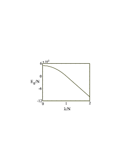
FIG. 1.: The ground state energy $E_{0}$ as a function of $\Lambda$ for $N=1000$ and $U_{1}=3U_{0}$ calculated for the two–mode model.

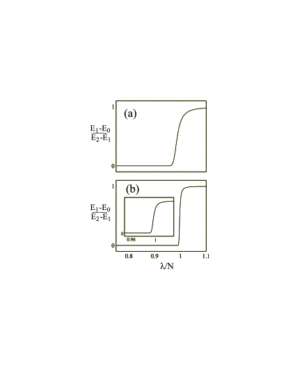
FIG. 2.: (a) The ratio between the energy difference of the first excited state and the ground state, and the energy difference of the second and first excited states $(E_{1}-E_{0})/(E_{2}-E_{1})$, as a function of $\Lambda$ for $U_{1}=3U_{0}$ and for $N=1000$; (b) Same as (a), but for $N=10000$. The inset shows the magnification of the transition region.

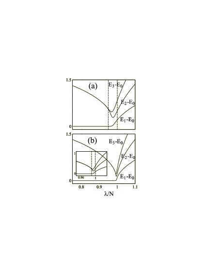
FIG. 3.: (a) The energy of the first, second and third excited states with respect to the energy of the ground state as a function of $\Lambda$ for $N=1000$, and other parameters the same as in Fig. 1. The dashed lines mark approximately the transition region; (b) Same as (a), but for $N=10000$. The inset shows the magnification of the transition region.

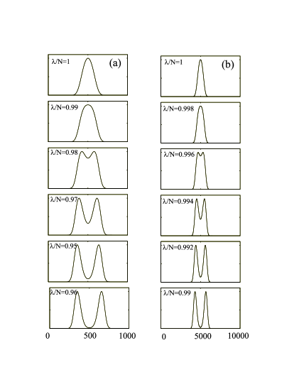
FIG. 4.: (a) $A$-atom number distributions for the ground state (i.e. the coefficients $|q_{m}^{0}|^{2}$ from Eq. (42) as a function of $m$) for $N=1000$ for the values of $\Lambda$ indicated. These values belong to the transition region between the dashed lines in Fig. 3(a); (b) Same as (a), but for $N=10000$. The values of $\Lambda$ belong to the transition region between the dashed lines in Fig. 3(b).

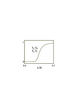
FIG. 5.: The energy difference of the first excited state and the ground state, and the energy difference of the second and first excited states $(E_{1}-E_{0})/(E_{2}-E_{1})$, as a function of $\Lambda$ for $N=1000$ and $U_{1}=3U_{0}$, calculated for the complete quantum field theoretical model. The parameters are: $a^{\rm sc}_{A}=a^{\rm sc}_{B}=50$ nm, $a^{\rm sc}_{AB}=150$ nm, $x_{0}=3$ $\mu$m, $\hbar\omega=100$ Hz

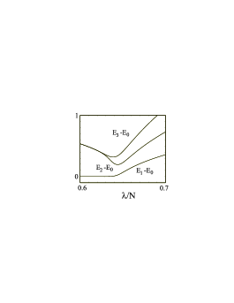
FIG. 6.: The energy of the first, second and third excited states with respect to the energy of the ground state as a function of $\Lambda$ calculated for the complete quantum field theoretical model. The parameters are the same as in Fig. 5.

REFERENCES

- [1] M. H.Anderson, J. R. Ensher, M. R. Matthews, C. E. Wieman, and E. A. Cornell, Science 269, 198 (1995).
- [2] K. B. Davis, M.-O. Mewes, M. R. Andrews, N. J. van Druten, D. S. Durfee, D. M. Kurn, and W. Ketterle, Phys. Rev. Lett. 75, 3969 (1995).
- [3] C. C. Bradley, C. A. Sackett, and R. G. Hulet, Phys. Rev. Lett. 78, 985 (1997).
- [4] For a review see: A. Griffin, D. W. Snoke, and S. Stringari, eds., Bose-Einstein Condensation (Cambridge, New York, 1995).
- [5] For a review see: J. Mlynek, V.Balykin, and P. Meystre (Eds.), Optics and Interferometry with Atoms, special issue of Appl. Phys. B54, 1992.
- [6] G. Lenz, P. Meystre, and E. M. Wright, Phys. Rev. Lett. 71, 3271 (1993); W. Zhang, D. F. Walls, and B. C. Sanders, Phys. Rev. Lett. 72, 60 (1994).
- [7] M. Edwards, P. A. Ruprecht, K. Burnett, and C. W. Clark, Phys. Rev. A, in print (1996).
- [8] For a review see: M. Lewenstein and L. You, in B. Bederson and H. Walther, eds., Adv. in Atom. Molec. and Opt. Phys. 36, 221 (1996).
- [9] Ch. J. Bordé, Phys. Lett. A204, 217 (1995); H. M. Wiseman and M. J. Collet, Phys. Lett. A202, 246 (1995); R. J. C. Spreeuw, T. Pfau, U. Janicke, and M. Wilkens, Europhys. Lett. 32, 469 (1995); M. Holland, K. Burnett, C. Gardiner, J. I. Cirac, and P. Zoller, Phys. Rev. A 54, R1757 (1996); M. Olshan’ii, Y. Castin, and J. Dalibard, in M. Ignuscio, M. Allegrini, and A. Lasso, eds., Proc. 12-th Int. Conference on Laser Spectroscopy, (World scientific, Singapour, 1995).
- [10] M.-O. Mewes, M. R. Andrews, D. M. Kurn, D. S. Durfee, C. G. Townsend, and W. Ketterle, Phys. Rev. Lett. 78, 582 (1997); M. R. Andrews, C. G. Townsend, H.-J. Miesner, D. S. Durfee, D. M. Kurn, and W. Ketterle, Science 275, 637 (1997).
- [11] J. F. Potayos, J. I. Cirac, and P. Zoller, Phys. Rev. Lett. 77, 4728 (1996).
- [12] D. S. Jin, J. R. Ensher, M. R. Matthews, C. E. Wieman, and E. A. Cornell, Phys. Rev. Lett. 77, 420 (1996); M.-O. Mewes, M. R. Andrews, N. J. van Druten, D. M. Kurn, D. S. Durfee, C. G. Townsend, and W. Ketterle, ibid., 988 (1996).
- [13] R. Walsworth and L. You, Harvard-Smithsonian Center for Astrophysics, preprint No. 4478, submitted to Phys. Rev. A (1997).
- [14] C. Monroe, D. M. Meekhof, B. E. King, and D. J. Wineland, Science 272, 1131 (1996).
- [15] M. Brune, E. Hagley, J. Dreyer, X. Maître, A. Maali, C. Wunderlich, J. M. Raimond, and S. Haroche, Phys. Rev. Lett. 77, 4887 (1996).
- [16] E. Schrödinger, Naturwissenschaften 23, 807, 823, 844 (1935).
- [17] J. von Neumann, Mathematische Grundlagen der Quantenmechanik, (Springer, Berlin, 1932).
- [18] J. A. Wheeler and W. H. Żurek, Quantum Theory and Measurement, (Princeton University Press, Princeton, 1983).
- [19] W. H. Żurek, Phys. Today 44, 36 (1991); W. H. Żurek, Phys. Rev. D24, 1516 (1981); ibid. 26, 1862 (1982); A. O. Caldeira and A. J. Leggett, Physica 121A, 587 (1983); E. Joos and H. D. Zeh, Z. Phys. B59, 223 (1985); R. Omnès, The Interpretation of Quantum Mechanics, (Princeton University Press, Princeton, 1994).
- [20] T-L. Ho and V. B. Shenoy, Phys. Rev. Lett. 77, 3276 (1996).
- [21] B. D. Esry and C. H. Greene, preprint (1997).
- [22] T. Busch, J. I. Cirac, V. Garia-Perez, and P. Zoller, submitted to Phys. Rev. A.
- [23] C. J. Myatt, E. A; Burt, R. W. Ghrist, E. A. Cornell, and C. E. Wieman, Phys. Rev. lett. 78, 586 (1997).
- [24] For a review see: W. Ketterle and N. J. van Druten, in B. Bederson and H. Walther, eds., Adv. in Atom. Molec. and Opt. Phys. 37, 181 (1996).
- [25] see for instance, M. Lewenstein, J. I. Cirac, and P. Zoller, Phys. Rev. A51, 4617 (1995), and references therein.
- [26] P. S. Julienne, F. H. Mies, E. Tiesinga, and C. J. Williams, Phys. Rev. Lett. 78, 1880 (1997); see also J. P. Burke, Jr., J. L. Bohn, B. D. Esry, and C. H. Greene, in print PHys. Rev. A (1997).
- [27] P. O. Fedichev, Yu. Kagan, G. V. Shlyapnikov, and J. T. M. Walraven, Phys. Rev. Lett. 77, 2913 (1996) and references cited.
- [28] H. Stoof, private communication.
- [29] G. Baym and C. J. Pethick, Phys. Rev. Lett. 76, 6 (1996).
- [30] R. Walser, unpublished; E. L. Bolda, S. M. Tan, D. F. Walls, quant-ph/9703014.