Quantum Statistical Thermodynamics of Two-Level Systems

Abstract

We study four distinct families of Gibbs canonical distributions defined on the standard complex, quaternionic, real and classical/nonquantum two-level systems. The structure function or density of states for any system is a simple power (1, 3, 0 or -1) of the length of its polarization vector, while the magnitude of the energy of the system, in all four cases, is the negative of the logarithm of the determinant of the corresponding $2\times 2$ density matrix. Functional relationships — proportional to ratios of gamma functions — are found between the average polarizations with respect to the Gibbs distributions and the effective polarization temperature parameters. In the standard complex case, this yields an interesting alternative, meeting certain probabilistic requirements recently set forth by Lavenda, to the more conventional (hyperbolic tangent) Brillouin function of paramagnetism (which, Lavenda argues, fails to meet such specifications).

I Introduction

In a number of forcefully-written papers some twenty years ago, Band and Park [1, 2, 3, 4] strongly recommended that the basic objective of quantum statistical thermodynamics should be taken to be the estimation of a Gibbs distribution (satisfying imposed constraints on expectation values of observables) over the continuum or “logical spectrum” of possible density matrices describing the system in question. This was viewed as a conceptually preferable alternative to that of estimating such a distribution over simply a set of eigenstates — corresponding to a single canonical density matrix — as in the standard Jaynesian approach [5, 6]. They, however, encountered “two barriers” in attempting to establish that their suggested methodology would yield identically the same expectation values as the empirically successful Jaynesian strategy. “One is essentially philosophical: The prior distribution needed in this continuum problem because of the inadequacy of the Laplacian rule of indifference, remains unknown. The other obstacle is mathematical: $\dots$ we could not perform the required integrals because we have no useful analytical description of the domain [of density matrices] and its boundary” [3, p. 235]. More recently, Park [7] (cf. [8]), in studying Schrödinger’s probability relations, wrote that the “details of quantum thermodynamics are presently unknown” and “perhaps there is more to the concept of thermodynamic equilibrium than can be captured in the canonical density operator itself.”

The first and principal model considered here (sec II A) is a particular implementation for the case of two-level (standard complex) quantum systems of the general program (formulated in terms of systems of arbitrary dimensionality) of Band and Park (cf. [9]). It yields seemingly novel analyses of both the thermodynamic properties of a plane radiation field [10] and of paramagnetic phenomena (cf. [11, 12, 13, 19]). A noteworthy aspect of our analyses is that we find it necessary to identify the parameter $\beta$ of the Gibbs distributions introduced below, not with the inverse thermodynamic temperature, as is conventional, but rather with the effective polarization temperature [10, 22]. Asymptotically, we find a negative log-linear relationship (equation (42) and Fig. 1) between this temperature and the reduced thermodynamic temperature of the standard model of paramagnetism.

The usual textbook treatment of the particular (spin-1/2) case of paramagnetism in which an ensemble of $n$ noninteracting two-level systems is subjected to a magnetic field $H$ predicts that the equilibrium magnetization ($M$) is given by the corresponding (hyperbolic tangent) Brillouin function, [14, p. 192],

$$M_{0}\tanh{\mu H\over kT},$$ (1)

where $M_{0}$ is the saturation magnetization, $\mu$ is the Bohr magneton, $k$ is Boltzmann’s constant and $T$ is temperature. Brillouin (generalized Langevin) functions, in general, it appears, yield good predictions except for low temperatures and high fields [16]. In volume I of his text, Balian [19, sec. 1.4.3] writes that the hyperbolic tangent Brillouin “model gives a qualitative understanding of the saturation effect…However, the quantitative agreement is not good as the behaviour predicted…altogether does not have the same shape as the experimental curves” (cf. [20, Fig. 6.5]).

Lavenda [14, p. 193] has recently argued that the hyperbolic tangent “Brillouin function has to coincide with the first moment of the distribution [for a two-level system having probabilities ${e^{x}\over e^{x}+e^{-x}}$ and ${e^{-x}\over e^{x}+e^{-x}}$], and this means that the generating function is $Z(x)=\cosh x$ [where $x={\mu H\over kT}$]. Now, it will be appreciated that this function cannot be written as a definite integral, such as

$$Z(\beta)={1\over 2}\int_{-1}^{1}e^{\beta x}dx={\sinh\beta\over\beta}=({\pi\over 2\beta})^{1/2}I_{1/2}(\beta),$$ (2)

because the integral form for the hyperbolic Bessel function,

$$I_{\nu}(x)={(x/2)^{\nu}\over\sqrt{\pi}\Gamma({1\over 2}+\nu)}\int_{-1}^{1}{e^{\pm xt}\sin^{\nu-1/2}tdt}$$ (3)

exists only for $\nu>{1\over 2}$. This means that $I_{-1/2}(x)=(2/{\pi x})^{1/2}\cosh x$ cannot be expressed in the above integral form. Since the generating function cannot be derived as the Laplace transform of a prior probability density, it casts serious doubts on the probabilistic foundations of the Brillouin function. In other words, any putative expression for the generating function must be compatible with the underlying probabilistic structure; that is, it must be able to be represented as the Laplace transform of a prior probability density.”

Additionally, as the concluding paragraph of his recent book, Lavenda writes [14, p. 198], “Even in this simple case of the Langevin function,

$$M=M_{0}\{\coth({\mu H\over kT})-{kT\over\mu H}\},$$ (4)

we have witnessed a transition from a statistics dictated by the central-limit theorem, at weak-fields, to one governed by extreme-value distributions, at strong-fields. Such richness is not possessed by the Brillouin function, for although it is almost identical to the Langevin function in the weak-field limit, the Brillouin function becomes independent of the field in the strong-field limit. In the latter limit, it would imply complete saturation which does not lead to any probability distribution. This is yet another inadequacy of modeling ferromagnetism by a Brillouin function, in the mean field approximation. And it is another illustration of our recurring theme that physical phenomena are always connected to probability distributions. If the latter does [sic] not exist, the former is [sic] almost sure to be illusory.”

We derive here standard complex, quaternionic, real and classical/nonquantum counterparts — (36), (52), (56) and (67) — to the hyperbolic tangent Brillouin function (1), which are, evidently, not subject to the objections to it that Lavenda has raised. The question of whether or not they are superior in explaining physical phenomena, warrants further investigation.

II Analyses of Four Types of Two-Level Systems

A The standard complex case

1 Gibbs canonical distributions

We consider the two-level quantum systems, describable (in the standard complex case) by $2\times 2$ density matrices of the form,

$$\rho={1\over 2}\pmatrix{\ 1+z&x-iy\cr x+iy&1-z\cr},\qquad(x^{2}+y^{2}+z^{2}\leq 1).$$ (5)

We assign to such a system an energy $(E)$ equal (in appropriate units) to the negative of the logarithm of the determinant of $\rho$, that is (transforming to spherical coordinates — $r,\theta,\phi$ — so that $x=r\cos\phi\sin\theta,y=r\sin\phi\sin\theta$ and $z=r\cos\theta$),

$$E=-\log(1-r^{2})$$ (6)

(cf. [11]). The radial coordinate ($r$) represents the degree of purity (the length of the polarization vector) of the associated two-level system. The pure states — $r=1$ — are assigned $E=\infty$, while the fully mixed state — $r=0$ — receives $E=0$. We, then, have (6),

$$r=\pm\sqrt{1-e^{-E}}.$$ (7)

We employ the positive branch of this solution as the density of states or structure function,

$$\Omega(E)=\sqrt{1-e^{-E}}\qquad(0\leq E\leq\infty).$$ (8)

(For small values of $E$, this is approximately $\sqrt{E}$.) The integrated density of states [15] is, then,

$$N(E_{0})=\int_{0}^{E_{0}}\Omega(E)=2(\tanh^{-1}\Omega(E_{0})-\Omega(E_{0})).$$ (9)

Inverting this relationship (cf. (1)), we have

$$\Omega(E_{0})=\tanh{{N(E_{0})+2\Omega(E_{0})\over 2}},$$ (10)

which for large $E_{0}$, yields

$$\Omega(E_{0})\approx\tanh{{N(E_{0})+2\over 2}}.$$ (11)

The Gibbs distributions having $\Omega(E)$ as their structure function are

$$f(E;\beta)={e^{-\beta E}\over Z(\beta)}\Omega(E)\qquad(0\leq\beta\leq\infty),$$ (12)

where $\beta$ is the effective polarization temperature parameter [10] and

$$Z(\beta)={\sqrt{\pi}\Gamma(\beta)\over 2\Gamma(3/2+\beta)}$$ (13)

serves as the partition function. In general, the zeros of a partition function are of special interest [17]. In this regard, let us note that the numerator of $Z(\beta)$ can not assume the value zero, since the gamma function has no zeros in the complex plane, although either its real or imaginary parts can vanish [18]. However, the denominator of $Z(\beta)$ assumes infinite magnitude at the [isolated] points $\beta=-3/2,-5/2,-7/2,\dots$, since $\Gamma(x)$ has simple poles at $x=-n,\quad n=0,1,2,\dots$ with residues $(-1)^{n}/n!$

We can compute the average or expected value of $E$, as

$$\langle E\rangle=-{\partial\over\partial\beta}\log Z(\beta)=\psi(3/2+\beta)-\psi(\beta)=\sum_{1}^{\infty}{(3/2)_{n}\over n(3/2+\beta)_{n}},$$ (14)

where the digamma function, $\psi(z)={d\over dz}{\log\Gamma(z)}={\Gamma^{\prime}(z)\over\Gamma(z)}$. (The last equality in (14), employing the Pochhammer symbol $(\lambda)_{n}$ is taken from [21], where it is also shown that this series can be written in terms of a generalized hypergeometric ${}_{3}F_{2}$ series.) For small values of $\beta$, we have

$$\beta\approx{1\over\langle E\rangle-2-\log 2}.$$ (15)

For large values of $\beta$,

$$\beta\approx{3\over 2\langle E\rangle}.$$ (16)

This can be understood from the fact that the digamma function satisfies the functional equation,

$$\psi(1+\beta)-\psi(\beta)={1\over\beta},$$ (17)

or, more formally, from the asymptotic ($\beta\rightarrow\infty$) expansion of $\langle E\rangle=\psi(3/2+\beta)-\psi(\beta)$,

$${3\over 2\beta}-{3\over 8\beta^{2}}+{1\over 4\beta^{3}}-{9\over 64\beta^{4}}+{1\over 16\beta^{5}}+O({1\over\beta^{6}}).$$ (18)

(It is highly interesting to note that one obtains the maximum-likelihood estimator $\hat{\beta}=3/{2\langle E\rangle}$ for an ideal monatomic gas, for which the logarithm of the partition function is $-{3\over 2}\log\beta$ [24, p. 468].) The variance of $E$ — that is, $\langle(E-\langle E\rangle)^{2}\rangle$ — is given by

$$\mbox{var}(E)={\partial^{2}\over\partial\beta^{2}}\log Z(\beta)=\psi^{\prime}(\beta)-\psi^{\prime}(3/2+\beta){\approx{3\over 2\beta^{2}}}\qquad(\beta\rightarrow\infty).$$ (19)

Interchanging the roles of $E$ and $\beta$ [23, 24, 25, 26], we obtain a (modal, as opposed to maximum likelihood [23]) estimate of the effective polarization temperature parameter $\beta$,

$${\partial\over\partial E}\log\Omega(E)={1\over 2(e^{E}-1)}.$$ (20)

Also, we have that

$$-{\partial^{2}\over\partial E^{2}}\log\Omega(E)={e^{E}\over 2(e^{E}-1)^{2}}.$$ (21)

2 Approximate duals of the Gibbs canonical distributions

The square root of (19) is the indicated (minimally informative Bayesian) prior over the parameter $\beta$ [24]. It is most interesting to note that as $\beta\rightarrow\infty$, this is proportional to $1/\beta$. The prior $1/\beta$ has arisen in several thermodynamic models and “is none other than Jeffreys’ improper prior for $\beta$ based on the invariance property that the prior be invariant with respect to powers of $\beta$” [24] or “the result obtained by Jeffreys for a scale parameter” [26]. The dual distribution (now regarding $E$ as the parameter to be fixed, rather than $\beta$) can then be written approximately (due to the use of (16)) as [26]

$$\tilde{f}(\beta;\langle E\rangle)\approx{3e^{-\beta E}\sqrt{\mbox{var}(E)}Z({3\over 2\langle E\rangle})\over 2Z(\beta)}.$$ (22)

As an example of this (approximate) duality, we have set $\langle E\rangle=16.3$ in (22) and divided the result by .984296 to obtain a probability distribution over $\beta\in[0,\infty]$. The expected value of $\beta$ was, then, found to be .0636579. Substituting this value into (14), we obtain an $\langle E\rangle$ of 16.2805 — which is near to 16.3. (For an initial choice of $\langle E\rangle<16.3$, we would expect the duality to be more exact in nature.) Now, in general,

$${\langle\beta\rangle}\approx{{\partial\over\partial\langle E\rangle}\log Z({3\over 2\langle E\rangle})}={3\over 2{\langle E\rangle}^{2}}(\psi({3\over 2}+{3\over 2\langle E\rangle})-\psi({3\over 2\langle E\rangle}))\approx{3\over 2\langle E\rangle}$$ (23)

and

$${\mbox{var}(\beta)}\approx{-{\partial^{2}\over\partial{\langle E\rangle}^{2}}\log Z({3\over 2\langle E\rangle})}$$

$$={3\over 4{\langle E\rangle}^{4}}(4\langle E\rangle(\psi({3\over 2}+{3\over 2\langle E\rangle})-\psi({3\over 2\langle E\rangle}))+3(\psi^{\prime}({3\over 2}+{3\over 2\langle E\rangle})-\psi^{\prime}({3\over 2\langle E\rangle})))\approx{3\over 2{\langle E\rangle}^{2}}\qquad(\langle E\rangle\rightarrow 0).$$ (24)

(The variance of $\beta$ for an ideal gas of $N$ particles is ${3N\over 2{\langle E\rangle}^{2}}$ [25, p. 207].) The square root of var($\beta$), which is approximately proportional to ${1\over\langle E\rangle}$ (again, in conformity to Jeffreys’ rule for a scale parameter), then, serves as the prior over $\langle E\rangle$ [24, eq. 21]. Following [24, eq. 27a], we can alternatively attempt to express the prior over $\langle E\rangle$ as the product of $\Omega(\langle E\rangle)$ and the reciprocal of $Z({3\over 2\langle E\rangle})$. We have plotted this result along with ${1\over\langle E\rangle}$ and both curves display quite similar monotonically decreasing behavior.

3 Thermodynamic interpretation of information-theoretic results of Krattenthaler and Slater

We have been led to advance the model (8)-(13) on the basis of results reported in [27] and subsequent related analyses. In [27], a one-parameter family (denoted $q(u)$) of probability distributions over the three-dimensional convex set (the “Bloch sphere” [28], that is, the unit ball in three-space) of two-level quantum systems (5) was studied. It took the form

$$q(u)={\Gamma(5/2-u)r^{2}\sin\theta\over\pi^{3/2}\Gamma(1-u)(1-r^{2})^{u}}\qquad(-\infty<u<1).$$ (25)

We note that the Gibbs distributions (12) can be obtained from (25) through the pair of changes-of-variables $u=1-\beta$ and $r=\sqrt{1-e^{-E}}=\Omega(E)$ (which is the positive branch of (7)), accompanied by integration over the two angular coordinates ($0\leq\theta<\pi,0\leq\phi<2\pi$). (We will in sec. II B use this pair of transformations also in the quaternionic, real and classical counterparts of the standard complex analysis.) In Cartesian coordinates, $q(u)$ takes the form

$${\Gamma(5/2-u)\over\pi^{3/2}\Gamma(1-u)(1-x^{2}-y^{2}-z^{2})^{u}}$$ (26)

Making the substitutions $X=x^{2},Y=y^{2}$ and $Z=z^{2}$, this becomes a Dirichlet distribution [29],

$${\Gamma(5/2-u)\over\pi^{3/2}\Gamma(1-u)\sqrt{X}\sqrt{Y}\sqrt{Z}(1-X-Y-Z)^{u}},$$ (27)

over the three-dimensional probability simplex spanned by the possible values of $X,Y$ and $Z$. (“In Bayesian statistics the Dirichlet distribution is known as the conjugate distribution of the multinomial distribution…In this sense the discrete coherent states are the quantum conjugate states of the Bose-Einstein symmetric number states” [30, Remark 2.3.3].)

The initial motivation for studying the family (25) in [27] was that it contained as a specific member — $q(.5)$ — a probability distribution (the “quantum Jeffreys prior”) proportional to the volume element of the Bures metric [31] on the Bloch sphere. (It now appears that all those values of $u$ lying between .5 and 1.5, or equivalently $\beta\in$ [-.5,.5], correspond to such “monotone” metrics [32, 33]. The desirability of monotone metrics stems from the finding that an “infinitesimal statistical distance has to be monotone under stochastic mappings” [34, p. 486].) We were interested in [27] (cf. [35]) in the possibility (in analogy to certain classical/nonquantum results of Clarke and Barron [36]) that the distribution $q(.5)$ might possess certain information-theoretic minimax and maximin properties vis-à-vis all other probability distributions over the Bloch sphere. However, considerations of analytical tractability led us to examine only those distributions in the family $q(u)$.

In [27], the probability distributions $q(u)$ were used to average the $n$-fold tensor products $(\stackrel{{\scriptstyle n}}{{\otimes}}\rho)$ over the Bloch sphere, thereby obtaining a one-parameter family of $2^{n}\times 2^{n}$ averaged matrices, $\zeta_{n}(u)$. The eigenvalues of $\zeta_{n}(u)$ were found to be

$$\lambda_{n,d}={1\over 2^{n}}{\Gamma(5/2-u)\Gamma(2+n-d-u)\Gamma(1+d-u)\over{\Gamma(5/2+n/2-u)\Gamma(2+n/2-u)\Gamma(1-u)}},\qquad d=0,1,\dots,\lfloor{\frac{n}{2}}\rfloor$$ (28)

with respective multiplicities,

$$m_{n,d}={(n-2d+1)^{2}\over(n+1)}{n+1\choose d}.$$ (29)

(Parallel analyses have also been conducted using the real analogue, $q_{real}(u)$, given by formula (53), of the standard complex probability distribution $q(u)$. However, it has proved more difficult, in this case, to give a formal demonstration of the validity of the derived expressions for the corresponding eigenvalues and eigenvectors.)

The subspace — spanned by all those eigenvectors associated with the same eigenvalue $\lambda_{n,d}$ — corresponds to those explicit spin states [37, sec. 7.5.j] [38] with $d$ spins either “up” or “down” (and the other $n-d$ spins, of course, the reverse). The $2^{n}$-dimensional Hilbert space can be decomposed into the direct sum of carrier spaces of irreducible representations of $SU(2)\times S_{n}$. The multiplicities (29) are the dimensions of the corresponding irreps. The $d$-th space consists of the union of ${m_{n,d}\over(n-2d+1)}$ copies of irreducible representations of SU(2), each of dimension $(n-2d+1)$ or, alternatively, of $(n-2d+1)$ copies of irreps of $S_{n}$, each of dimension ${m_{n,d}\over(n-2d+1)}$.

In [27], an explicit formula, in terms of the eigenvalues, (28) was obtained for the relative entropy of $\stackrel{{\scriptstyle n}}{{\otimes}}\rho$ with respect to $\zeta_{n}(u)$,

$$-nS(\rho)-\mbox{Tr}(\stackrel{{\scriptstyle n}}{{\otimes}}\rho\cdot\log\zeta_{n}(u)),$$ (30)

where $S(\rho)=-\mbox{Tr}\rho\log\rho$ is the von Neumann entropy of $\rho$. Then, the asymptotics of this quantity (30) was found as $n\rightarrow\infty$. We can now reexpress this result ([27, eq. 2.36]) in terms of the thermodynamic variables ($\beta,E$), rather than $r$ and $u$, as (using the positive branch of (7))

$${3\over 2}\log n-{1\over 2}-{3\over 2}\log 2+\beta E+{1\over 2\Omega(E)}\log[{1-\Omega(E)\over 1+\Omega(E)}]+\log\Gamma(\beta)-\log\Gamma({3\over 2}+\beta)+O({1\over n}).$$ (31)

Let us naively (that is, ignoring the error term immediately above) attempt to find an asymptotically stationary point of the relative entropy (30) by setting the derivatives of (31) with respect to $\beta$ and $E$ to zero, and then numerically solving the resultant pair of nonlinear simultaneous equations. The derivative with respect to $\beta$ simply yields the condition (14) — that is, the likelihood equation — that $E=\langle E\rangle$, while that with respect to $E$ can be expressed as

$$\beta={1\over 4\Omega(E)^{2}}(2+{1\over e^{E}\Omega(E)}\log[{1-\Omega(E)\over 1+\Omega(E)}]).$$ (32)

We obtained a stationary value of the truncated asymptotics (31) at the point ($\beta=.457407,E=2.58527$). It appears possible that this point serves as an asymptotic minimax for the relative entropy. Though additional numerical evidence appears consistent with such a proposition, a formal demonstration remains to be given. In [27], the asymptotics of the maximin — with respect to the one-parameter family — of the relative entropy was formally found. (This involved integrating out the radial coordinate $r$. In this analysis, it was possible to show that it was harmless to ignore the error term in (31).) It corresponded to the value $\beta=.468733$. This was obtained as the solution of an equation [27, eq. (3.10)], here expressible as

$$2\beta^{3}\mbox{var}(E)=1.$$ (33)

(Use of $\mbox{var}(E)\approx{3\over 2\beta^{2}}$ from (19) in this equation would give a solution of $\beta={1\over 3}$.) It is interesting to note that both the [rather proximate] values of $\beta$ of .457407 and .468733 lie in the range [-.5,.5] associated with monotone metrics [32]. In their classical/nonquantum analysis, Clarke and Barron [36] found that both the asymptotic minimax and maximin were given by the very same probability distribution — the Jeffreys prior, which is based on the unique monotone metric in that classical domain of study.

Let us note — in view of the forms of expression of (31) and (32) — that in [10, eq. (2.4)] (cf. [22]) the expression

$${1\over 2}\log[{1+\Omega(E)\over 1-\Omega(E)}]={1\over 2}\log[{1+r\over 1-r}]\approx r+{r^{3}\over 3}+{r^{5}\over 5}+\ldots$$ (34)

was taken to be the reciprocal ($\tau^{-1}$) of “an effective polarization temperature ($\tau$) [which] should not be confused with the radiance temperature obtained using Planck’s spectral law”. (The equality in (34) will not hold in the quaternionic and real cases discussed below (sec. II B), since then the structure function will not simply equal the radial coordinate.) Inverting equation (2.4) of [10], we obtain

$$r={e^{2/\tau}-1\over e^{2/\tau}+1}=\tanh{{1\over\tau}}$$ (35)

(cf. formulas (1.28) and (1.36) of [6]). It will be of substantial interest (setting $\tau=\beta$) to compare (35) with the relations we obtain — (36), (52) and (56) — for the average polarization $\langle r\rangle$ as a function of $\beta$. This will be done in Fig. 2.

4 Dependence of the average polarization upon the parameter $\beta$

The expected value of the structure function $\Omega(E)$, that is (8) — equal to the radial coordinate ($r$) — with respect to the family of Gibbs distributions (12) is exactly computable. We have that

$$\langle r\rangle=\langle{\Omega(E)}\rangle={1\over\beta(1+\beta)Z(\beta)}={2\Gamma(3/2+\beta)\over\beta(1+\beta)\sqrt{\pi}\Gamma(\beta)}={2\Gamma(3/2+\beta)\over\sqrt{\pi}\Gamma(2+\beta)}$$ (36)

For small values of $\beta$ (cf. (15)),

$$\beta\approx{1-\langle r\rangle\over 2\log 2-1}.$$ (37)

Asymptotically, $\beta\rightarrow\infty$,

$$\langle r\rangle={1\over\sqrt{\pi}}({2\over\beta^{1/2}}-{5\over 4\beta^{3/2}}+{73\over 64\beta^{5/2}}-{575\over 512\beta^{7/2}})+O({1\over\beta^{9/2}}).$$ (38)

We have found a series of curves for integral $n$ that converges (as C. Krattenthaler has formally demonstrated) to (36) as $n\rightarrow\infty$ (cf. [39]). The curves are obtained by summing the weighted terms $(n-2d)/n$ over the $1+\lfloor n/2\rfloor$ subspaces (indexed by $d$) of explicit spin states, using as the weights, the probabilities assigned to the subspaces, that is, the product of the eigenvalue ($\lambda_{n,d}$) for the $d$-th subspace (28) and its associated multiplicity ($m_{n,d}$) (29). Thus, we consider

$$\sum_{d=0}^{\lfloor n/2\rfloor}({n-2d\over n})m_{n,d}\lambda_{n,d}.$$ (39)

This gives the average or expected polarization (since $n-2d$ is the net spin for $n-d$ majority spins assigned $+1$ and $d$ minority spins assigned $-1$), ranging between 0 and 1. (There have been recent studies [41, 42] of the temperature dependence of the average spin polarization in a system — a quantum Hall ferromagnet — in which the spins are not [as assumed here] noninteracting (cf. [43]).) Thus, similarly to the parameter $\tau$ in [10], the value $\beta=0$ corresponds to complete polarization (total domination by the majority spin) and $\beta=\infty$ to the case in which there is no predominance of spin in any direction.

The convergence of the sum (39) to the mean value (36) has been essentially demonstrated by Krattenthaler by, first, rewriting (39) as the difference

$$\sum_{d=0}^{\lfloor n/2\rfloor}({n-2d+1\over n})m_{n,d}\lambda_{n,d}-\sum_{d=0}^{\lfloor n/2\rfloor}({1\over n})m_{n,d}\lambda_{n,d}.$$ (40)

(His proof — applicable to any probability distribution over the Bloch sphere which is spherically-symmetric — is conducted in terms of the spherical coordinates used in [27], but it easily carries over to the presentation here in terms of the thermodynamic variables, $\beta$ and $E$.) He shows — employing Theorem 15 of [27] to reexpress $\lambda_{n,d}$, then splitting the resulting expression into four terms, in the manner of (2.41)-(2.46) of [27] and applying the binomial theorem — that (40) and, hence, (39) can be rewritten as the sum of the expected value of $q(u)$ (that is, ${2\Gamma(5/2-u)\over\sqrt{\pi}\Gamma(3/2-u)}$) and a term that converges to zero as $n\rightarrow\infty$.

5 Relations between average polarization (36) and hyperbolic tangent Brillouin (1) functions

Let us, in the obvious task of trying to relate the results here to the conventionally employed hyperbolic tangent Brillouin function (1), equate the reduced magnetization [11] given by ${M\over M_{0}}=\tanh{{\mu H\over kT}}$ to the average polarization $\langle r\rangle$ obtained from formula (36). To do so, we set the reduced temperature ($x\equiv{\mu H\over kT})$ equal to $\tanh^{-1}\langle r\rangle$. Asymptotically then, as $\beta\rightarrow\infty$, this gives

$$x={2\over\sqrt{\pi}\sqrt{\beta}}+{32-15\pi\over 12{\pi}^{3/2}{\beta}^{3/2}}+O({1\over{\beta}^{2}}).$$ (41)

Consequently, for large values of $\beta$, we have the log-linear approximation,

$$\log{x}\approx\log{2}-{1\over 2}\log{\pi}-{1\over 2}\log{\beta}=.120782-{1\over 2}\log{\beta}.$$ (42)

In Fig. 1, we plot $\log{\tanh^{-1}\langle r\rangle}$ vs. the logarithm of the effective polarization temperature $\beta$. For large $\beta$, the curve is approximately linear, having a slope of $-{1\over 2}$.

FIG. 1.: The Logarithm of the Inverse Hyperbolic Tangent of the Average Polarization (36) for the Standard Complex Model of sec. II A vs. the Logarithm of the Effective Polarization Temperature Parameter $\beta$. For large $\beta$, the curve is approximately linear with a slope of $-{1\over 2}$.

To further study the relationship of the results in this study to the standard treatment of paramagnetism (see also the formulas we obtain for the integrated density of states — (10), (48), (63)), in which the hyperbolic tangent Brillouin function (1) is employed [11, 12, 13, 19], it might prove useful to employ the relationships between the hyperbolic functions and the gamma functions in the complex plane [44, eqs. 6.1.23-6.1.32]. Pursuing this line, we have found that

$$\langle r\rangle{2\sqrt{\pi}(\beta+1)\Gamma(3/2-\beta)\over(4{\beta}^{2}-1)\Gamma(-\beta)}=i\tanh{\pi\beta\over i}=\tan\beta\pi.$$ (43)

Error bounds for the asymptotic expansion of the ratio of two gamma functions with complex argument (cf. (13) and (36)) have been given in [45] (extending earlier work [46] on the ratio of two gamma functions with real argument), using generalized Bernoulli polynomials (cf. [47]).

B Cases other than the standard complex

Although quantum mechanics is usually treated as a theory over the algebraic field of complex numbers, it is also possible and of considerable interest to study versions over the real and quaternionic fields, as well [48, 49]. The possibility of testing these different forms against one another has been studied [50, 51, 52]. It appears that the results here — giving distinct Gibbs distributions in the three quantum mechanical scenarios — may present another avenue to addressing such fundamental issues.

1 Quaternionic case

For the quaternions, the analogue of the probability distribution $q(u)$ given in (25) takes the form (cf. [49, eq. 26]),

$$q_{quat}(u)={\Gamma(7/2-u)r^{4}{\sin}^{3}\theta_{1}{\sin}^{2}\theta_{2}\sin\theta_{3}\over\pi^{5/2}\Gamma(1-u)(1-r^{2})^{u}}\qquad(-\infty<u<1),$$ (44)

being defined over the five-dimensional unit ball or “quaternionic Bloch sphere.” Proceeding with the same transformations as in the standard complex case — that is, $u=1-\beta$ and $r=\sqrt{1-e^{-E}}$ — and integrating over the four angular coordinates, we arrive at a family of Gibbs distributions (12) having as their structure function or density of states (cf. (8)),

$$\Omega_{quat}(E)=\Omega_{complex}^{3}(E)=(1-e^{-E})^{3\over 2}$$ (45)

(which is approximately $E^{3/2}$ for small $E$), where $\Omega_{complex}(E)\equiv\Omega(E)=\sqrt{1-e^{-E}}$, from (8). The integrated density of states (cf. (9)) is, then,

$$N_{quat}(E_{0})=\int_{0}^{E_{0}}\Omega_{quat}(E)=2(\tanh^{-1}\Omega_{complex}(E_{0})+{\Omega_{complex}(E_{0})(1-4e^{E_{0}})\over 3e^{E_{0}}}),$$ (46)

Also, we have the difference,

$$N_{complex}(E_{0})-N_{quat}(E_{0})={2\Omega_{complex}(E_{0})(e^{E_{0}}-1)\over 3e^{E_{0}}}.$$ (47)

As $E_{0}\rightarrow\infty$, it approaches from below, the limiting value of ${2\over 3}$. For large $E_{0}$ (cf. (1), (11)),

$$\Omega_{complex}(E_{0})\approx\tanh{{3N_{quat}(E_{0})+8\over 6}}.$$ (48)

The partition function (cf. (13)) in the quaternionic case is

$$Z_{quat}(\beta)={3\sqrt{\pi}\Gamma(\beta)\over 4\Gamma(5/2+\beta)}.$$ (49)

We now have (cf. (14))

$${\langle E_{quat}\rangle}=-{\partial\over\partial\beta}\log Z_{quat}(\beta)=\psi(5/2+\beta)-\psi(\beta)\approx{5\over 2\beta}\qquad(\beta\rightarrow\infty)$$ (50)

and (cf. (19))

$$\mbox{var}_{quat}(E)={\partial^{2}\over\partial{\beta}^{2}}\log Z_{quat}(\beta)=\psi^{\prime}(\beta)-\psi^{\prime}(5/2+\beta)\approx{5\over 2{\beta}^{2}}\qquad(\beta\rightarrow\infty).$$ (51)

It, thus, appears that the quaternionic results relating to approximate duality can, in essence, be obtained from the (standard complex) ones given above (sec. II A 2), simply through the substitution of ${5\over 2}$ for ${3\over 2}$, as appropriate. We have conducted a test of approximate duality similar to that reported (for the standard complex case) immediately after (22). We have set ${\langle E\rangle}_{quat}=16.3$ in the evident quaternionic analogue of (22), and divided the result by .902062 to obtain a probability distribution over $\beta\in[0,\infty]$. The expected value of $\beta$ was, then, found to be .0664174. Substituting this value into (50), we obtain an estimate of ${\langle E\rangle}_{quat}$ equal to 16.2645 $\approx$ 16.3.

For the average quaternionic polarization, we have

$${\langle r_{quat}\rangle}=\langle{\Omega_{quat}(E)}^{1/3}\rangle={8\Gamma(5/2+\beta)\over 3\beta(1+\beta)(2+\beta)(3+\beta)\sqrt{\pi}\Gamma(\beta)}={8\Gamma(5/2+\beta)\over 3\sqrt{\pi}\Gamma(3+\beta)}.$$ (52)

(It would appear problematical, however, to develop a quaternionic counterpart to the analysis of Krattenthaler and Slater [27], as there are difficulties in defining an appropriate extension of the tensor product [48].)

2 Real case

We can also, proceeding similarly, take

$$q_{real}(u)={2\Gamma(2-u)r\over\Gamma(1-u)(1-r^{2})^{u}}={(1-u)r\over\pi(1-r^{2})^{u}}\qquad(-\infty<u<1),$$ (53)

as a probability distribution over the unit (two-dimensional) disk. Integrating over the single angular coordinate and using the transformations, $u=1-\beta$ and $r=\sqrt{1-e^{-E}}$, we transform (53) to a Gibbs distribution, having a structure function $\Omega_{real}(E)\equiv 1$ and a partition function,

$$Z_{real}(\beta)={\Gamma(\beta)\over\Gamma(1+\beta)}={1\over\beta}.$$ (54)

(The integrated density of states is, of course, then, simply $N_{real}(E_{0})=E_{0}$.) Now (cf. (17)),

$$\langle E_{real}\rangle=-{\partial\over\partial\beta}\log Z_{real}(\beta)=\psi(1+\beta)-\psi(\beta)={1\over\beta}$$ (55)

So, it appears that the “fraction”’ $1={2\over 2}$ plays the analogous role in real quantum mechanics as ${3\over 2}$ in the standard complex version and ${5\over 2}$ in the quaternionic form. (These results appear consistent with the equipartition of energy theorem [53] in classical statistical mechanics, as two, three and five are the corresponding degrees of freedom, that is, the number of variables needed to fully specify a real, standard complex or quaternionic density matrix.)

The expected value of $r$ with respect to (53) (again using $u=1-\beta$) gives us the average polarization in the real case,

$${\langle r_{real}\rangle}={\sqrt{\pi}\Gamma(1+\beta)\over 2\Gamma(3/2+\beta)}.$$ (56)

The three forms of average polarization — (36), (52) and (56) — are particular instances of the formula,

$${\Gamma(1+m/2)\Gamma(1/2+\beta+m/2)\over\Gamma(1+\beta+m/2)\Gamma({1+m\over 2})},$$ (57)

where the quaternionic case corresponds to $m=4$, the standard complex to $m=2$ and the real to $m=1$.

3 Classical/nonquantum case

The case $m=0$ is, essentially classical/nonquantum in nature, corresponding to the family of probability distributions,

$$q_{class}(u)={2\Gamma(3/2-u)\over\sqrt{\pi}\Gamma(1-u)(1-r^{2})^{u}}\qquad(-\infty<u<1).$$ (58)

(If one makes the transformation $r=\sqrt{R}$, this becomes (cf. (27)) a family of beta distributions. Then, the member corresponding to $u={1\over 2}$, is the (bimodal) arcsine (alternatively, cosine [54]) distribution, corresponding to a process with a single degree of freedom, to which Boltzmann’s principle is inapplicable [55]. The arcsine distribution serves as the noninformative Jeffreys’ prior for the Bayesian inference of the parameter of a binomial distribution [56, 57].) Making the same substitutions as in the previous cases, that is $u=1-\beta$ and $r=\sqrt{1-e^{-E}}$, into (58), we obtain

$$\Omega_{class}(E)={1\over\Omega_{complex}(E)}={1\over\sqrt{1-e^{-E}}},$$ (59)

$$Z_{class}(\beta)={\sqrt{\pi}\Gamma(\beta)\over\Gamma(1/2+\beta)},$$ (60)

and

$$\langle E_{class}\rangle=-{\partial\over\partial\beta}\log Z_{class}(\beta)=\psi(1/2+\beta)-\psi(\beta)\approx{1\over 2\beta}\qquad(\beta\rightarrow\infty)$$ (61)

(corresponding to the single degree of freedom in this case). Also, setting $m=0$ in (57), we have

$$\langle r_{class}\rangle={\Gamma(1/2+\beta)\over\sqrt{\pi}\Gamma(1+\beta)}.$$ (62)

For the integrated density of states, we find $N_{class}(E_{0})=2\tanh^{-1}\Omega_{complex}(E_{0})$, so

$$\Omega_{complex}(E_{0})=\tanh{{N_{class}(E_{0})\over 2}}.$$ (63)

C Comparison of results for the four different cases

The average polarization indices for the four models considered above all equal 1 for $\beta=0$ and monotonically decrease to 0 for $\beta=\infty$. However, for $\beta$ strictly between 0 and $\infty$, the quaternionic value is always greater than the standard complex one, which, in turn, is always greater than the real index (which itself dominates the classical one). (In this regard, it may be helpful to note that the ratio of (52) to (36) simplifies to ${2(3+2\beta)\over 3(2+\beta)}$.)

In Fig. 2, we plot the average polarization as a function of $\beta$ for the quaternionic, standard complex, real and classical cases ($m=4,2,1$ and 0, respectively). We also display the Brosseau-Bicout relation (35), having set $\tau=\beta$. This last curve crosses the other four. It predicts greater average polarization in the vicinity of $\tau=\beta=0$ and less above a certain threshold (which is smallest in the quaternionic case and largest in the classical one).

FIG. 2.: Average Polarization as a Function of the Effective Polarization Temperature $\beta$. The quaternionic curve (52) dominates the standard complex curve (36), which, in turn, dominates the real curve (56). This dominates the classical/nonquantum curve (62)). The function of Brosseau and Bicout (35), setting $\tau=\beta$, making it equivalent to $\tanh{{1\over\beta}}$, crosses the four other curves, intersecting at $\beta$ = .76007, 1.04585, 1.46249 and 3.1857.

In Fig. 3, we plot the expected value $\langle E\rangle$ of the energy $E$ for the quaternionic, standard complex, real and classical cases, while in Fig. 4, we show the corresponding variances var($E$)..

FIG. 3.: Expected values $\langle E\rangle$ of the energy $E$. The order of dominance is $\langle E_{quat}\rangle>\langle E_{complex}\rangle>\langle E_{real}\rangle>\langle E_{class}\rangle$.

FIG. 4.: Variances of the energy $E$. The order of dominance is $\mbox{var}(E_{quat})>\mbox{var}(E_{complex})>\mbox{var}(E_{real})>\mbox{var}(E_{class})$.

D An alternative family of Gibbs canonical distributions for the standard complex case

In the analyses reported above, we have relied upon certain transformations of the probability distribution $q(u)$ (25), defined over the Bloch sphere of two-level systems, and its real (53) and quaternionic (44) analogues, to obtain the Gibbs distributions we have studied. The distribution $q(u)$ has the attractive feature that for $u\in[.5,1)$ (and also for $u\in[1,1.5]$, although $q(u)$ is improper in this range), it is proportional to the volume element of a monotone metric on the two-level systems. (The value $u=.5$ corresponds to the minimal [Bures] monotone metric and $u=1.5$ to the maximal one.)

Nevertheless, there appear to be alternatives to $q(u)$ that are of certain interest and might conceivably be physically meaningful. One such family of probability distributions can be expressed as [27, eq. (3.11)]

$$q_{KMB}(u)={(1-u)\Gamma(3/2-u)r\log[(1+r)/(1-r)]\sin\theta\over 2\pi^{3/2}\Gamma(1-u)(1-r^{2})^{u}}\qquad(-\infty<u<1).$$ (64)

For $u={1\over 2}$, this is proportional to the volume element of the Kubo-Mori/Bogoliubov (monotone) metric [34, 58, 59]. “This metric is infinitesimally induced by the (nonsymmetric) relative entropy functional or the von Neumann entropy of density matrices. Hence its geometry expresses maximal uncertainty” [34]. The family (64) can essentially be obtained from the family $q(u)$ by replacing a factor of $r$ by $\log[{(1+r)\over(1-r)}]$ and renormalizing the result. For values of $r$ in the neighborhood of 0, $q(u)$ and $q_{KMB}(u)$, for any fixed $u$, are approximately proportional (cf. (34)). (The KMB-metric is the extreme element [$\alpha=\pm 1$] of a one-parameter ($\alpha$) family — distinct from (64) — all the members of which correspond to monotone Riemannian metrics induced by quantum alpha-entropies [59]. However, the corresponding volume elements for $-1<\alpha<1$ do not appear to be exactly normalizable over the Bloch sphere of two-level systems.)

If we perform the transformations, $u=1-\beta$ and $r=\sqrt{1-e^{-E}}$, then (64) becomes a family of Gibbs distributions (12) with the partition function,

$$Z_{KMB}(\beta)={Z_{class}(\beta)\over\beta}={\sqrt{\pi}\Gamma(\beta)\over\beta\Gamma(1/2+\beta)},$$ (65)

and, quite interestingly, the structure function (cf. (34),

$$\Omega_{KMB}(E)=\log[{(1+\sqrt{1-e^{-E}})\over(1-\sqrt{1-e^{-E}})}$$

$$=2(\sqrt{1-e^{-E}}+{(1-e^{-E})^{3/2}\over 3}+\ldots)=2(\Omega_{complex}(E)+{\Omega_{quat}(E)\over 3}+\ldots).$$ (66)

Using the positive branch of (7), $\Omega_{KMB}(E)$ is simply twice the reciprocal ($\tau^{-1}$) of the effective polarization temperature ($\tau$), as defined by Brosseau and Bicout [10, eq. 2.4] (cf. (34)). The range of possible values of this structure function is the nonnegative real axis $[0,\infty]$, in contrast to the structure functions considered above, which only assume values on the unit interval [0,1]. We were able to explicitly compute the corresponding integrated density of states — but the expression MATHEMATICA 3.0 yielded was highly complicated. In Fig. 5, we have plotted the five integrated density of states functions obtained here — $N_{complex}(E_{0}),N_{quat}(E_{0}),N_{real}(E_{0})=E_{0},N_{class}(E_{0})$ and $N_{KMB}(E_{0})$.

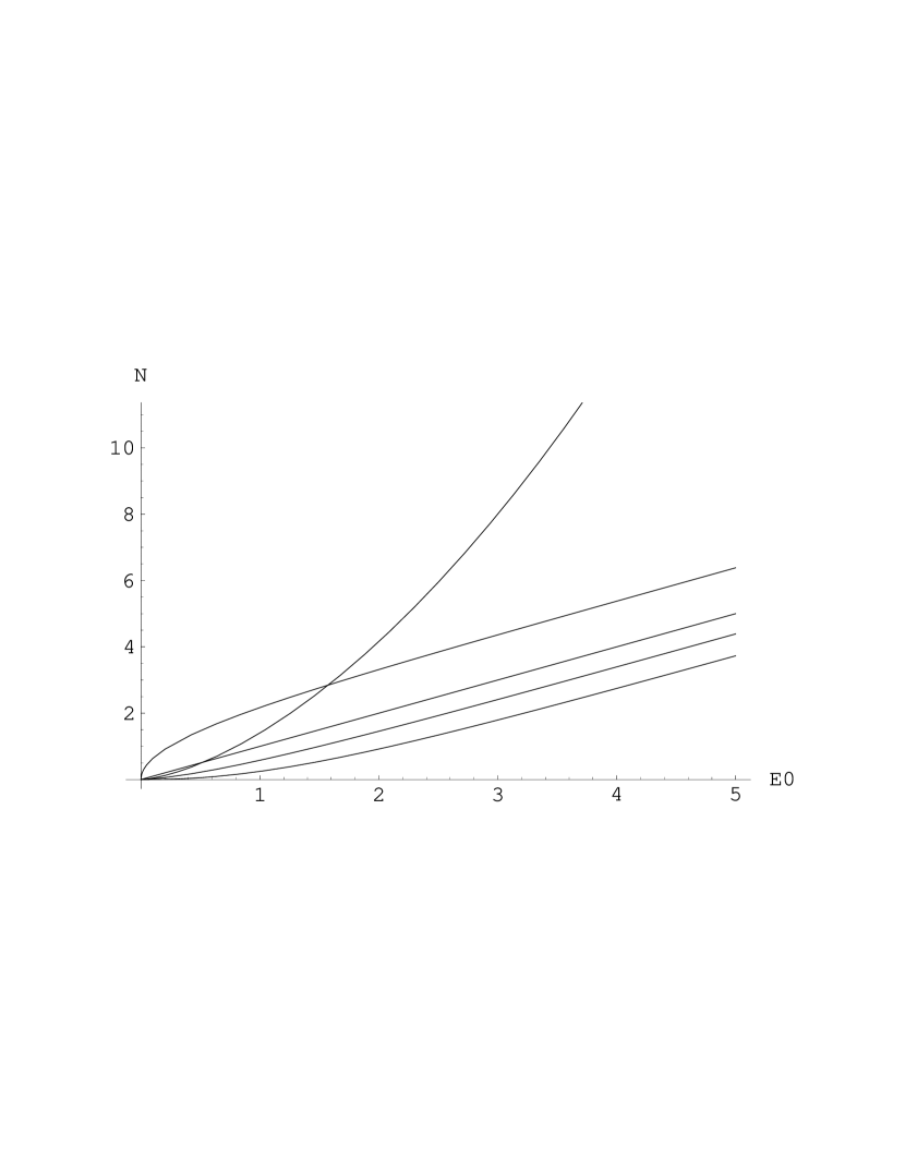
FIG. 5.: Integrated Densities of States for Five Different Models. The most steeply-rising curve corresponds to $N_{KMB}(E_{0})$, while the order of dominance for the other four curves is classical $>$ real $>$ standard complex $>$ quaternionic. The $KMB$-curve crosses the classical one at $E_{0}=1.57565$, the real linear one — $N_{real}(E_{0})=E_{0}$ — at .53341, the standard complex curve at .000111286, and the quaternionic curve at .0000405489. Asymptotically ($E_{0}\rightarrow\infty$), the difference (47), that is $N_{complex}(E_{0})-N_{quat}(E_{0})$, monotonically increases to its limit ${2\over 3}$.

The first term of the asymptotic expansion ($\beta\rightarrow\infty$) of $-{\partial\over\partial\beta}\log Z_{KMB}$ is ${3\over{2\beta}}$. This is the same as was found above (18) for the standard complex case and which coincides with the behavior of the ideal monatomic gas. The first term of the asymptotic expansion ($\beta\rightarrow\infty$) of the square root of ${\partial^{2}\over\partial{\beta}^{2}}\log Z_{KMB}$ is ${3\over 2\beta^{2}}$, again as in the standard complex case considered previously (19).

The expected value of $r$ with respect to (64) — giving us the average polarization index — can be expressed as

$${\langle r_{KMB}\rangle}={2\beta\Gamma(1/2+\beta)_{P}F_{Q}[\{{1\over 2},1,2\},\{{3\over 2},2+\beta\},1]\over\sqrt{\pi}\Gamma(2+\beta)}.$$ (67)

Due to its hypergeometric character, it is difficult to analytically study (67). A plot (Fig. 6) of the difference between it and the alternative (standard complex) average polarization index (36), shows that the latter index is dominated by (67), with the greatest difference ($\approx.0526$) occurring in the vicinity of $\beta=.49825$. (We have earlier indicated that for the distributions $q(u)$, given in (25), taking $u=1-\beta$, the range $\beta\in[-.5,.5]$ — which includes .49825 — parameterizes a continuum of monotone metrics.)

FIG. 6.: The average polarization given by $\langle r_{KMB}\rangle$ minus the average polarization $\langle r\rangle$ — given by (36), plotted in Fig. 2 — for the first/primary standard complex model considered here (sec. II A).

III Concluding Remarks

The Brillouin functions of paramagnetism serve as the basis of the mean-field theory of ferromagnetism [11, 12, 20]. It would, therefore, be of interest to construct mean-field theories based on the alternative functions that we have developed above. In this regard, following the usual line of argument [20, sec. 6.2] [60, sec. 9.2], we have replaced $\beta$ by $\beta/(\lambda\langle r\rangle)$ in the small-$\beta$ approximation (37) to the average polarization index (36) in the standard complex case. ($\lambda$ corresponds to the molecular field parameter.) Then, we find that there exists a nonzero critical effective polarization temperature,

$$\beta_{c}={\lambda\over 4(2\log{2}-1)}=.647175\lambda$$ (68)

below which spontaneous magnetization is possible. We are (using the same approximation and following [61, sec. 3.1]) able to construct an order parameter of the form

$$2\langle r\rangle-1=\pm(1-{\beta_{c}\over\beta})^{1/2}.$$ (69)

So, the exponent for the power law behavior of the order parameter is the same as for the hyperbolic tangent Brillouin function (1) [61, eq. (3.10)], that is the simple fraction ${1\over 2}$ — as is not actually the case for real ferromagnets. (Lavenda and Florio [62] assert that the probability density centered about the metastable state of the order parameter for the mean-field theory of the kinetic Weiss-Ising model is an asymptotic distribution for the smallest value, rather than a normal distribution, as generally assumed.)

The possibility of obtaining results analogous to those derived here, for $n$-level systems ($n>2$) should be investigated. Such results could, then, be compared with those given by the particular $n$-level form of the Brillouin function. In this regard, it might be of some relevance to note that Brosseau [63] has recently shown that the polarization entropy of a stochastic radiation field depends on ($n-1$) measures of the degree of polarization of the field.

If one considers the pure states in a $2m$-dimensional complex Hilbert space, endowed with the unitarily invariant integration measure [64], then tracing over $m$ degrees of freedom, one induces a probability distribution on the two-level standard complex quantum systems taking the form of the Gibbs distribution (12) with $\beta=m-1$ [65] (cf. [66]).

Boltzmann’s principle — $S=k\log\Omega$ + const —relates the entropy, $S$, to the logarithm of the thermodynamic probability, $\Omega$, of a given state [14, sec. II.4.1]. The question of whether this important principle has a meaningful application to the structure functions considered here ($\Omega_{complex},\Omega_{quat},\Omega_{real}\equiv 1$, $\Omega_{class}$ and $\Omega_{KMB}$) certainly merits investigation. (We note that all but the last of these functions assume the value 1 for $E=\infty$, the logarithm of which is 0 equaling, as would seem appropriate, the von Neumann entropy, $-\mbox{Tr}\rho\log\rho$, of a pure state — that is, one for which, $\det{\rho}=0$ or, equivalently, $r=1$ or $E=\infty$ (cf. (6)). However, the von Neumann entropy of the fully mixed state, corresponding to $r=0$ or $E=0$, is $\log 2$, not $-\infty$, as a naive application of the principle would, then, give.)

White [67] has developed a density matrix formulation for quantum renormalization groups and applied it to Heisenberg chains. (He shows that keeping the most probable eigenstates of the block density matrix gives the most accurate representation of the system as a whole, that is, the block plus the rest of the lattice.) We have indicated here a different use of the density matrix concept in studying spin systems, in line with the program expounded by Band and Park. In their series of papers [1, 2, 3, 4], they take exception to the Jaynesian strategy of maximization of the von Neumann entropy subject to constraints on expected values of observables [5, 6] and suggest that rather one should estimate a Gibbs distribution over the continuum or “logical spectrum” of possible density matrices. We should also point out, however, that Band and Park — in contrast to Lavenda [24, 25] and Tikochinsky and Levine [26] — do not discuss the notion of an (improper or nonnormalizable) structure function or density of states over the energy levels (such as we encounter here with (8), (45), (59), (66) and $\Omega_{real}(E)\equiv 1$), but solely that of a reparameterization-invariant prior probability distribution over the convex set of quantum systems (cf. [57]). Within the framework of their analysis, concerned with systems of arbitrary dimensionality (not simply two-dimensional systems, as here), Band and Park did conclude [3, 4] that for the case of “strong” or dynamical equilibrium, an axiom of “data indifference” was preferable to one of “state indifference”.

In conclusion, let us state that we have found counterparts (that is, the expected values $\langle r\rangle$ of the radial coordinate $r$ in the Bloch sphere-type representations of the two-level systems) — (36), (52), (56) and (67) — to the hyperbolic tangent Brillouin function (1), which are evidently not subject to the methodological objections of Lavenda [14]. Of particular novelty has been the identification of the parameter $\beta$ of the Gibbs canonical distributions introduced above with the effective polarization temperature, and not, as is conventional, the inverse thermodynamic temperature.

Further theoretical and empirical analyses pertaining to the potential applicability to physical phenomena of the results reported here would, indeed, appear appropriate.

- [1] J. L. Park and W. Band, Found. Phys. 6, 157 (1976).
- [2] W. Band and J. L. Park, Found. Phys. 6, 249 (1976).
- [3] J. L. Park and W. Band, Found. Phys. 7, 233 (1977).
- [4] W. Band and J. L. Park, Found. Phys. 7, 705 (1976).
- [5] E. T. Jaynes, Phys. Rev. 108, 171 (1957).
- [6] R. Balian and N. L. Balazs, Ann. Phys. (NY) 179, 97 (1987).
- [7] J. L. Park, Found. Phys. 18, 225 (1988).
- [8] E. P. Gyftopoulos and E. Çubukçu, Phys. Rev. E 55, 3851 (1997).
- [9] P. B. Slater, Phys. Lett. A 171, 285 (1992).
- [10] C. Brosseau and D. Bicout, Phys. Rev. E 50, 4997 (1994).
- [11] J. A. Tuszyński and W. Wierzbicki, Amer. J. Phys. 59, 555 (1991).
- [12] F. Schlögl, Probability and Heat (Friedr. Vieweg, Braunschweig, 1989).
- [13] E. V. Goldstein, Yu. Sadaui, and V. M. Tsukernik, Phys. Rev. E 47, 3749 (1993).
- [14] B. H. Lavenda, Thermodynamics of Extremes (Albion, West Sussex, 1995).
- [15] E. Brézin, D. J. Gross, and C. Itzykson, Nucl. Phys. B 235, 24 (1984).
- [16] E. Abrahams and F. Keffer, in McGraw-Hill Encyclopaedia of Science and Technology (McGraw-Hill, New York, 1977), vol. 13, p. 96.
- [17] K.-C. Lee, Phys. Rev. E 53, 6558 (1996).
- [18] J. Bohman and C.-E. Frőberg, Math. Comput. 58, 315 (1992).
- [19] R. Balian, From Microphysics to Macrophysics: Methods and Applications of Statistical Physics (Spinger, Berlin, 1991).
- [20] H. E. Stanley, Introduction to Phase Transitions and Critical Phenomena (Oxford, New York, 1971).
- [21] B. N. Al-Saqabi, S. L. Kaller, and H. M. Srivastava, J. Math. Anal. Appl. 159, 361 (1991).
- [22] C. Christodoulides, Phys. Stat. Sol. (a) 109, 611 (1988).
- [23] B. Mandelbrot, Phys. Today 42:1, 71 (1989).
- [24] B. H. Lavenda, Intl. J. Theor. Phys. 27, 451 (1988).
- [25] B. H. Lavenda, Statistical Physics (Wiley, New York, 1991).
- [26] Y. Tikochinsky and R. D. Levine, J. Math. Phys. 25, 2160 (1984).
- [27] C. Krattenthaler and P. B. Slater, Asymptotic Redundancies for Universal Quantum Coding, Los Alamos preprint archive, quant-ph/9612043 (1996).
- [28] S. L. Braunstein and G. J. Milburn, Phys. Rev. A 51, 1820 (1995).
- [29] T. S. Ferguson, Ann. Statist. 1, 209 (1973).
- [30] A. Bach, Indistinguishable Classical Particles (Springer, Berlin, 1997).
- [31] S. L. Braunstein and C. M. Caves, Phys. Rev. Lett. 72, 3439 (1994).
- [32] D. Petz and C. Sudar, J. Math. Phys. 37, 2662 (1996).
- [33] D. Petz, Lin. Alg. Applic. 244, 81 (1996).
- [34] D. Petz, J. Math. Phys. 35, 780 (1994).
- [35] P. B. Slater, J. Phys. A 29, L601 (1996).
- [36] B. S. Clarke and A. R. Barron, J. Statist. Plann. Inference 41, 37 (1994).
- [37] L. C. Biedenharn and J. D. Louck, Angular Momentum in Quantum Physics (Addison-Wesley, Reading, 1981).
- [38] R. Pauncz, Spin Eigenfunctions: Construction and Use (Plenum, New York, 1979).
- [39] E. Farhi and J. Goldstone, Ann. Phys. (NY) 192, 368 (1989).
- [40] M. J. Manfra et al, Phys. Rev. B 54, R17327 (1996).
- [41] T. Chakraborty and P. Pietiläinen, Phys. Rev. Lett. 76, 4018 (1996).
- [42] M. J. Manfra et al, Phys. Rev. B 54, R17327 (1996).
- [43] T. W. Riddle et al, J. Vac. Sci. Technol. 15, 1686 (1978).
- [44] Handbook of Mathematical Functions, edited by M. Abramowitz and I. A. Stegun (Dover, New York, 1972).
- [45] C. L. Frenzen, SIAM J. Math. Anal. 23, 505 (1992).
- [46] C. L. Frenzen, SIAM J. Math. Anal. 18, 890 (1987).
- [47] R. B. Paris and A. D. Wood, J. Comput. Appl. Math. 41. 135 (1992).
- [48] S. L. Adler, Quaternionic Quantum Mechanics and Quantum Fields (Oxford, New York, 1995).
- [49] P. B. Slater, J. Math. Phys. 37, 2682 (1996).
- [50] D. I. Fivel, Phys. Rev. A 50, 2108 (1994).
- [51] A. J. Davies and B. H. J. McKellar, Phys. Rev. A 46, 3671 (1992).
- [52] S. P. Brumby and G. C. Joshi, Chaos, Solitons and Fractals 7, 747 (1996).
- [53] L. E. Beghian, Nuovo Cim. B 107, 841 (1992).
- [54] G. M. D’Ariano and M. G. A. Paris, Phys. Rev. A 48, 4039 (1993).
- [55] B. H. Lavenda, Intl. J. Theor. Phys. 34, 605 (1995).
- [56] J. M. Bernardo and A. F. M. Smith, Bayesian Theory (Wiley, New York, 1994).
- [57] P. B. Slater, Noninformative Priors for Quantum Inference, Los Alamos preprint archive, quant-ph/9703012 (1997).
- [58] D. Petz and G. Toth, Lett. Math. Phys. 27, 205 (1993).
- [59] D. Petz and H. Hasegawa, Lett. Math. Phys. 38, 221 (1996).
- [60] R. Balescu, Equilibrium and Nonequilibrium Statistical Mechanics (Wiley, New York, 1975).
- [61] M. Plischke and B. Bergersen, Equilibrium Statistical Physics (World Scientific, Singapore, 1994).
- [62] B. H. Lavenda and A. Florio, Intl. J. Theor. Phys. 31, 1455 (1992).
- [63] C. Brosseau, Optik 104, 21 (1996).
- [64] K. R. W. Jones, Ann. Phys. (NY) 207, 140 (1991).
- [65] D. N. Page, Phys. Rev. Lett. 71, 1291 (1993).
- [66] R. Derka, V. Bužek, and G. Adam, Acta Phys. Slov. 46, 355 (1966).
- [67] S. R. White, Phys. Rev. B 48, 10345 (1993); Phys. Rev. Lett. 69, 2863 (1992).