Gamow-Jordan Vectors and Non-Reducible Density Operators from Higher Order S-Matrix Poles

Abstract

In analogy to Gamow vectors that are obtained from first order resonance poles of the S-matrix, one can also define higher order Gamow vectors which are derived from higher order poles of the S-matrix. An S-matrix pole of $r$-th order at $z_{R}=E_{R}-i\Gamma/2$ leads to $r$ generalized eigenvectors of order $k=0,~{}1,\ldots,~{}r-1$, which are also Jordan vectors of degree $(k+1)$ with generalized eigenvalue $(E_{R}-i\Gamma/2)$. The Gamow-Jordan vectors are elements of a generalized complex eigenvector expansion, whose form suggests the definition of a state operator (density matrix) for the microphysical decaying state of this higher order pole. This microphysical state is a mixture of non-reducible components. In spite of the fact that the $k$-th order Gamow-Jordan vectors has the polynomial time-dependence which one always associates with higher order poles, the microphysical state obeys a purely exponential decay law.

1 Introduction

The singularities of the analytically continued S-matrix that have attracted most of the attention in the past are the first order poles in the second sheet. They were associated with resonances that decay exponentially in time. [1] In conventional Hilbert space quantum theory it was not clear what those resonance “states” were, since a vector description of a resonance state was not possible within the framework of the Hilbert space.[2] Higher order poles, in particular double poles have also been mentioned, but it has long been believed that they somehow lead to an additional polynomial time dependence of the decay law [3]. However, precise derivations were not possible due to the lack of a vector space description.

This changed when the first order poles were associated with vectors ${\psi^{G}=\sqrt{2\pi\Gamma}|E_{R}-i\Gamma/2\rangle}$ in a rigged Hilbert space (RHS) [4, 5, 6, 7], called Gamow vectors. They possess all the properties that one needs to describe decaying states or resonances: These Gamow vectors $\psi^{G}$ are eigenvectors of a self-adjoint Hamiltonian [8] with complex eigenvalues $z_{R}=E_{R}-i\Gamma/2$ (energy and width). They evolve exponentially in time, and they have a Breit-Wigner energy distribution. They also obey an exact Golden Rule, which becomes the standard Golden Rule if one replaces $\psi^{G}$ with its Born approximation. The existence of these vectors allows us to interpret resonances as autonomous physical systems (which one cannot do in standard quantum mechanics). It also puts quasibound states (i.e. resonances) and anti-bound (or virtual) states [6] on the same footing with the bound states (eigenvectors with real energy), which have both a vector description and an S-matrix description. Mathematically, Gamow vectors are a generalization of Dirac kets (describing scattering states), i.e. they are also eigenkets. But whereas Dirac kets are associated with a value of the continuous Hilbert space spectrum of the self-adjoint Hamiltonian $H$, the Gamow kets are not, but have complex eigenvalues.

Using the entirely different theory of finite dimensional complex matrices, decaying states (like the $K^{0}-\bar{K}^{0}$ system) have been phenomenologically described as eigenvectors of an effective Hamiltonian matrix with complex eigenvalues. One usually assumes that these complex Hamiltonians are diagonalizable [9]. However, unlike hermitean matrices which have real eigenvalues, non-hermitean finite dimensional matrices cannot always be diagonalized, but can only be brought into a Jordan canonical form [10]. Finite dimensional matrices consisting of non-diagonalizable Jordan blocks have been mentioned in connection with resonances numerous times in the past [11, 12, 13, 14, 15], and they have been used for discussions of problems in nuclear [14] and in hadron [15] physics. Jordan blocks have also been obtained in prototypes of mixing systems [13], and the appearance of so-called “irreducible” non-diagonalizable blocks in the density matrix has been sought after for some time in connection with irreversible thermodynamics and the approach to equilibrium [16]. That irreducible non-diagonalizable Jordan blocks may shed light on the idea of quantum chaos has been mentioned by Brändas and Dreismann [12]. Also important for the understanding of quantum chaos and of the statistical properties of nuclear spectra are accidental degeneracies and level crossing, which in the past had been almost exclusively restricted to stable systems driven by hermitean Hamiltonians [17]. Based on a finite dimensional phenomenological expression for the S-matrix [18], Mondragón et al. [14] extended these discussions to resonance states described by a Jordan block of rank $2$.

In the present paper we shall show that the Jordan blocks emerge naturally for the matrix elements $\,{}^{(k)}\langle^{-}z_{R}|H|\psi^{-}\rangle$ of a self-adjoint [8] Hamiltonian $H$ between Gamow vectors $|z^{-}_{R}\rangle^{(k)}$ of order $k=1,~{}2,\dots,r-1$. From the generalized basis vector expansion derived here it follows that these $r$-dimensional blocks are a truncation of the infinite dimensional exact theory in the RHS.

The higher order Gamow vectors $|z^{-}_{R}\rangle^{(k)}$ have been derived in a recent unpublished preprint by Antoniou and Gadella [19]. The derivation is a generalization of the method by which the Gamow vector (of order $k=0$) was derived from the first order poles of the S-matrix [5]. Starting from an $r$-th order pole of the S-matrix element at complex energy $z=z_{R}$, they derived $r$ Gamow vectors of higher order, $|E_{R}-i\Gamma/2\,^{-}\rangle^{(k)}$, $k=0,\,1,\cdots r-1$, as functionals in a rigged Hilbert space. These higher order Gamow kets are also Jordan vectors belonging to the eigenvalue $z_{R}$.

In the present paper we generalize the RHS theory of the Gamow vectors associated with first order S-matrix poles, which we call Gamow vectors of order zero, to poles of order $r$. Quasistationary states in scattering experiments (i.e. states formed if the projectile is temporarily captured by the target) can be shown to appear not only as first order poles, but as poles of any order $r=1,2,\dots$ ([3]). In section 2, we will start from the expression for the unitary S-matrix of a quasistationary state of finite order $r$ and energy $E_{R}$, given in reference [4] sect. XVIII.6, and obtain from it $r$ Gamow vectors of order $k=0,1,\dots,r-1$ which are also Jordan vectors of degree $k+1$. After a review of the case $r=1$ in section 3, we derive in section 4 the generalized eigenvector expansion, which contains the Gamow-Jordan vectors as basis vectors. With these basis vectors we can give a matrix representation of $H$ and of $e^{-iHt}$ which contains the $r$-dimensional Jordan blocks. In section 5, we start from the pole term of the $r$-th order S-matrix pole and conjecture the state operator for the hypothetical microphysical system associated with this pole. This $r$-th order Gamow state operator consists of non-diagonalizable blocks which obey a purely exponential decay law. This unexpected result is in contrast to the belief [3] that higher order poles must lead to an additional polynomial time dependence.

At the present time there is little empirical evidence for the existence of these higher order pole “states” in nature. This is in marked contrast to the fact that first order pole states described by ordinary Gamow vectors have been identified in abundance, e.g. through their Breit-Wigner profile in scattering experiments and through their exponential decay law.

Now that our results have obliterated the prime empirical objection of non-exponentiality against the existence of higher order pole states, one can continue to look for them. The first step in this direction is to use these higher order state operators in the exact Golden Rule [4] and obtain the decay probability and the decay rate, including the line widths. We plan to do this in a forthcoming paper.

2 Poles of the S-matrix and Gamow-Jordan Vectors

Since the new (hypothetical) states are to be defined by the $r$-th order pole of the S-matrix, we consider a scattering system. The S-matrix consists of the matrix elements [21]

$$\left(\psi^{\text{out}},\phi^{\text{out}}\right) =\left(\psi^{\text{out}}(t),\phi^{\text{out}}(t)\right)=\left(\psi^{\text{out}},S\phi^{\text{in}}\right)$$

$$=\left(\Omega^{-}\psi^{\text{out}}(t),\Omega^{+}\phi^{\text{in}}(t)\right)=\left(\psi^{-}(t),\phi^{+}(t)\right)=\left(\psi^{-},\phi^{+}\right)$$ (2.1)

$$=\int_{\text{spectrum }H}dE\;\langle\psi^{-}|E^{-}\rangle S(E+i0)\langle^{+}E|\phi^{+}\rangle\;.$$

Since we are interested only in the principles here, in equation (2.1) (and in subsequent equations) we choose to ignore all other labels of the basis vectors $|E^{\pm}\rangle$ and $|E\rangle$ except the energy label $E$, which can take values on a two-sheeted Riemann surface. Nothing principally new will be gained if we retain the additional quantum numbers $b=b_{2},\,b_{3},\ldots b_{\cal N}$ in the basis system $|E^{\pm}\rangle\Longrightarrow|E,b^{\pm}\rangle=|E,\,b_{2},\,b_{3},\,\ldots b^{\pm}_{\cal N}\rangle$, and in place of the integral over the energy we would just have some additional sums (or integrals in the case that some of the $b$’s are continuous) over the quantum numbers $b$. For instance, if one chooses the angular momentum basis $|E^{\pm}\rangle\Longrightarrow|E,l,\,l_{3},\,\eta^{\pm}\rangle$, where $\eta$ are some additional (polarization or) channel quantum numbers (cf. [4], sect.  XX.2, XXI.4), then (2.1) would read in detail

$$\left(\psi^{-},\phi^{+}\right)= \sum_{l,\,l_{3},\,\eta}\sum_{l^{\prime},\,l^{\prime}_{3},\,\eta^{\prime}}\iint\,dE\,dE^{\prime}\,\langle\psi^{-}\,|\,E^{\prime},\,l^{\prime},\,l^{\prime}_{3},\,\eta^{\prime-}\rangle\times$$ (2.2)

$$\quad\times\langle^{-}E^{\prime},\,l^{\prime},\,l^{\prime}_{3},\,\eta^{\prime}\,|E,\,l,\,l_{3},\,\eta^{+}\rangle\langle^{+}E,\,l,\,l_{3},\,\eta\,|\,\phi^{+}\rangle\;.$$

Restricting ourselves to one initial $\eta=\eta_{A}$ and one final $\eta^{\prime}=\eta_{B}$ channel (e.g., $\eta_{B}=\eta_{A}$ for elastic scattering) we obtain

$$\langle^{-}E^{\prime},l^{\prime},l^{\prime}_{3},\eta_{B}|E,l,l_{3},\eta_{A}^{+}\rangle = \langle E^{\prime},l^{\prime},l^{\prime}_{3},\eta_{B}|\,S\,|E,l,l_{3},\eta_{A}\rangle$$

$$= \delta(E^{\prime}-E)\delta_{l^{\prime}_{3}l_{3}}\delta_{l^{\prime}l}\langle\eta_{B}|\!|S|\!|\eta_{A}\rangle$$

where

$$\langle\eta_{B}\,|\!|\,S\,|\!|\,\eta_{A}\rangle=S^{\eta_{B}}_{l}(E)$$ (2.4)

is the $l$-th partial S-matrix element for scattering from the channel $\eta_{A}$ into one particular channel $\eta_{B}$ (e.g., the elastic channel, $\eta_{B}=\eta_{A}$). If we consider the $l$-th partial wave of the $\eta_{B}$-th channel, then the $S(E)$ in (2.1) is given by this matrix element $S(E)=S^{\eta_{B}}_{l}(E)$. E.g., if we consider a mass point in a potential barrier, then $|E^{\pm}\rangle=|E,\,l,\,l^{\pm}_{3}\rangle$ is the angular momentum basis of the mass point and, depending on the shape and height of the barrier, one or several resonances can exist. Many concrete examples have been studied where one can see how first order resonance poles $z_{R_{i}}=E_{R_{i}}-i\,\Gamma_{i}/2$ move as a function of the potential parameters [22]. We want to consider just one pole, and in the present paper we are mainly interested in a higher order pole at $z_{R}$. Whether physical systems exist that are described by higher order poles is not clear, but a few examples of second order poles have been discussed in the past [3] [14].

With the above simplifications to one channel $\eta_{B}$ and one partial wave $l$, the notation in (2.1) is standard in scattering theory.

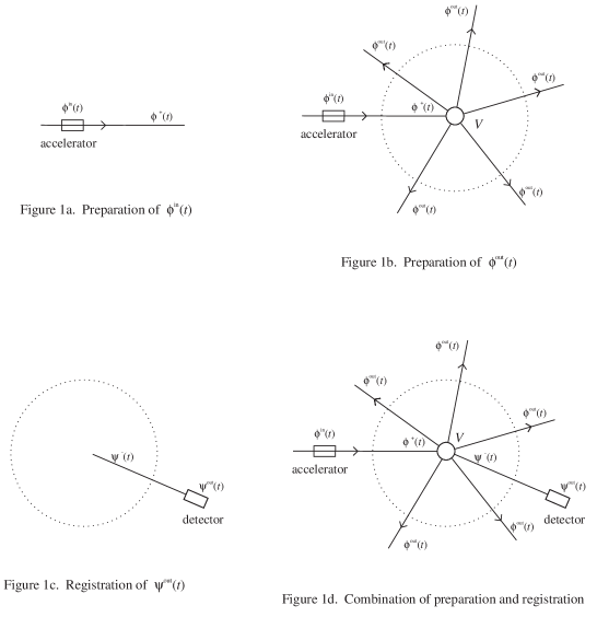
Figure 1: The preparation-registration procedure in a scattering experiment

The standard scattering theory uses the same Hilbert space ${\cal H}$ for both the set of in-states $\phi^{+}$ and the set of out-“states” $\psi^{-}$. The RHS formulation allows us to use two RHS’s for the set $\{\phi^{+}\}$ defined by the initial conditions and the set $\{\psi^{-}\}$ defined by the final conditions. To explain this we subdivide the scattering experiment into a preparation stage and a registration stage, as explained in detail in reference [23]. Fig. 1 depicts these different stages illustrating the idealized process: The in-state $\phi^{+}$ (precisely the state which evolves from the prepared in-state $\phi^{\text{in}}$ outside the interaction region where $V=H-H_{0}$ is zero) is determined by the accelerator. The so-called out-state $\psi^{-}$ (or $\psi^{\text{out}}$) is determined by the detector; $|\psi^{\text{out}}\rangle\langle\psi^{\text{out}}|$ is therefore the observable which the detector registers and not a state. In the conventional formulation one describes both the $\phi^{\text{in}}$ and the $\psi^{\text{out}}$ by any vectors of the Hilbert space. In reality the $\phi^{\text{in}}$ (or $\phi^{+}$) and $\psi^{\text{out}}$ (or $\psi^{-}$) are subject to different initial and boundary conditions and are therefore described by different sets of vectors belonging to different rigged Hilbert spaces. The RHS for the Dirac kets is denoted by

$$\Phi\subset{\cal H}\subset\Phi^{\times}$$ (2.5)

where $\Phi$ is the space of the “well-behaved” vectors (Schwartz space), and the Dirac kets (scattering states) $|E^{\pm}\rangle$ and $|E\rangle$ are elements of $\Phi^{\times}$. The in-state vectors $\phi^{+}(t)=e^{iHt/\hbar}\phi^{+}$ evolve from the prepared in-state $\phi^{\text{in}}(t)=(\Omega^{+})^{-1}\,\phi^{+}(t),\,t<0,$ and the out-observable vectors $\psi^{-}(t)=e^{iHt/\hbar}\psi^{-}$ evolve into the measured out-state $\psi^{\text{out}}(t)=(\Omega^{-})^{-1}\,\psi^{-}(t),\,t>0$.[24]

We denote the space of $\{\phi^{+}\}$ by ${\Phi}_{-}$ and the space of $\{\psi^{-}\}$ by ${\Phi}_{+}$. Then, ${\Phi}={\Phi}_{-}+{\Phi}_{+}$, where ${\Phi}_{-}\cap{\Phi}_{+}\neq\emptyset$. In place of the single rigged Hilbert space (2.5), one therefore has a pair of rigged Hilbert spaces:

$$\phi^{+}\in\;{\Phi}_{-}\subset{\cal H}\subset{\Phi}^{\times}_{-}&\text{for in-states of a scattering}\\ \text{experiment which are prepared}\\ \text{by a preparation apparatus,}\\ \psi^{-}\in\;{\Phi}_{+}\subset{\cal H}\subset{\Phi}^{\times}_{+}\text{for observables or out-``states''}\\ \text{which are registered by a detector.}$$ (2.6)

The Hilbert space ${\cal H}$ in (2.5), (2.6a), and (2.6b) is the same, but ${\Phi}_{+}$ and ${\Phi}_{-}$ are two distinct spaces of “very well-behaved” vectors. The spaces ${\Phi}_{+}$ and ${\Phi}_{-}$ can be defined mathematically in terms of the spaces of their wave functions $\langle^{+}E|\phi^{+}\rangle$ and $\langle^{-}E|\psi^{-}\rangle$, respectively. This is the realization of these abstract spaces by spaces of functions, in very much the same way as the Hilbert space ${\cal H}$ is realized by the space of Lebesgue square-integrable functions $L^{2}[0,\infty)$. The space ${\Phi}_{-}$ is realized by the space of well-behaved Hardy class functions in the lower half-plane of the second energy sheet of the S-matrix $S(E)$, and the space ${\Phi}_{+}$ is realized by the space of well-behaved Hardy class functions in the upper half-plane. Thus, the mathematical definition of the spaces $\Phi_{+}$ and $\Phi_{-}$ is:

$$\psi^{-}\in{\Phi}_{+}\quad\text{iff}\quad\langle\,E\,|\,\psi^{\text{out}}\rangle=\langle^{-}E\,|\psi^{-}\rangle\in{\cal S}\cap{\cal H}^{2}_{+}\,\Bigr{|}_{{\rm{I\!R}}^{+}}$$ (2.7)

and

$$\phi^{+}\in\Phi_{-}\quad\text{iff}\quad\langle\,E\,|\,\phi^{\text{in}}\rangle=\langle^{+}E\,|\phi^{+}\rangle\in{\cal S}\cap{\cal H}^{2}_{-}\,\Bigr{|}_{{\rm{I\!R}}^{+}}\;.$$ (2.8)

Here ${\cal S}$ denotes the Schwartz space and ${\cal S}\cap{\cal H}^{2}_{\pm}$ is the space of Hardy class functions from above/below. This mathematical property of the spaces ${\Phi}_{+}$ and ${\Phi}_{-}$ can be shown to be a consequence of the arrow of time inherent in every scattering experiment [23].

Being Hardy class from below means that the analytic continuation $\langle\psi^{-}|z^{-}\rangle$ of $\langle\psi^{-}|E^{-}\rangle=\overline{\langle^{-}E|\psi^{-}\rangle}$, and the analytic continuation $\langle^{+}z|\phi^{+}\rangle$ of $\langle^{+}E|\phi^{+}\rangle$, and therewith also $\langle\psi^{-}|z^{-}\rangle\langle^{+}z|\phi^{+}\rangle$, are analytic functions in the lower half-plane which vanish fast enough on the lower infinite semicircle. (For the precise definition, see [7, 25]). The values of a Hardy class function in the lower half-plane are already determined by its values on the positive real axis [26]. From (2.7) and (2.8) follows that

$$\langle\psi^{-}|E^{-}\rangle\langle^{+}E|\phi^{+}\rangle\in{\cal S}\cap{\cal H}^{p}_{-}\;,\;p=1$$ (2.9)

and so are all its derivatives

$$\bigl{(}\langle\psi^{-}|E^{-}\rangle\langle^{+}E|\phi^{+}\rangle\bigr{)}^{(n)}\in{\cal S}\cap{\cal H}^{p}_{-}\;;\hskip 14.45377ptp=1,~{}n=0,\,1,\,2,\,\ldots$$ (2.10)

because the derivation is continuous in ${\cal S}$.

With the above preparations one can derive the vectors that are associated with the $r$-th order pole of the S-matrix for any value of $r$, in complete analogy to the derivation of the vectors associated with the first order poles, $r=1$.[5]     We shall see that there are $r$ generalized vectors of order $k=0,\,1,\ldots,\,r-1$ associated with an $r$-th order pole. We call these vectors the higher order Gamow vectors, or Gamow-Jordan vectors (since they also have the properties of Jordan vectors [10]). Their first derivation from the $r$-th order pole was given in [19]. Here we give an alternative derivation and discuss their properties and applications in the generalized basis vector expansion.

We consider the model in which the analytically continued S-matrix $S(\omega)$ has one $r$-th order pole at the position $\omega=z_{R}$ ($z_{R}=E_{R}-i\,\Gamma/2$) in the lower half-plane of the second sheet, (and consequently there is also one $r$-th order pole in the upper half-plane of the second sheet at $\omega=z^{\ast}_{R}$). In this paper we will not discuss the pole at $z^{\ast}_{R}$. It leads to $r$ growing higher order Gamow vectors and the correspondence between the growing and decaying vectors is just the same as for the case $r=1$. The model that we discuss here can easily be extended to any finite number of finite order poles in the second sheet below the positive real axis.

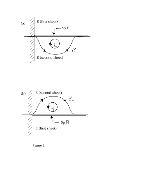
Figure 2: The contours in the two sheeted Riemann surface. (a) displays the contour ${\cal C}^{-}$ that results from extending the spectrum of the Hamiltonian ${\rm Sp}(\bar{H})={\rm{I\!R}}^{+}$ into the lower half-plane of the second Riemann sheet and that yields the pole term in eq. (2.14) at the position $z_{R}=(E_{R}-i\Gamma/2)$. (b) displays the extension of the contour into the upper half-plane of the second sheet with pole at $z^{*}_{R}$, which we shall not discuss here any further; it leads to the growing higher order Gamow vectors.

The unitary S-matrix of a quasistationary state associated with an $r$-th order pole at $z_{R}=E_{R}-i\Gamma/2$ is represented in the lower half-plane of the second sheet by ([4] sect. XVIII.6)

$$S_{\rm II}(\omega) = e^{2ir\;{\rm arctan}(\frac{\Gamma}{2(E_{R}-\omega)})}e^{2i\gamma(\omega)}=\left(\frac{\omega-E_{R}-i\Gamma/2}{\omega-(E_{R}-i\Gamma/2)}\right)^{r}e^{2i\gamma(\omega)}$$ (2.11)

$$= \left(1+\frac{-i\Gamma}{\omega-(E_{R}-i\Gamma/2)}\right)^{r}e^{2i\gamma(\omega)}\;.$$

Here, $\delta_{R}(\omega)=2ir\,{\rm arctan}(\frac{\Gamma}{2(E_{R}-\omega)})$ is the rapidly varying resonant part of the phase shift, and $\gamma(\omega)$ is the background phase shift, which is a slowly varying function of the complex energy $\omega$. We have restricted ourselves to the case that the $r$-th order pole is the only singularity of the S-matrix. Below we will mention how this can be generalized to the case of a finite number of finite order poles. (Note that phenomenologically only a finite number of first order poles have been established, but there is no theoretical reason that would prevent other isolated singularities on the second sheet below the real axis.)

For our calculations we have to write (2.11) in the form of a Laurent series:

$$S_{\rm II}(\omega) = \sum_{l=-r}^{+\infty}C_{l}(\omega-z_{R})^{l}$$

$$= \frac{C_{-r}}{(\omega-z_{R})^{r}}+\frac{C_{-r+1}}{(\omega-z_{R})^{r-1}}+\dots+C_{0}+C_{1}(\omega-z_{R})+\dots$$

Therefore we expand the bracket in (2.11):

$$S_{\rm II}(\omega) = \left(\sum_{l=0}^{r}\begin{pmatrix}r\\ l\end{pmatrix}\frac{(-i\Gamma)^{l}}{(\omega-z_{R})^{l}}\right)e^{2i\gamma(\omega)}$$

$$= e^{2i\gamma(\omega)}+\sum_{l=1}^{r}\begin{pmatrix}r\\ l\end{pmatrix}\frac{(-i\Gamma)^{l}}{(\omega-z_{R})^{l}}e^{2i\gamma(\omega)}$$

$$= e^{2i\delta_{R}(\omega)}e^{2i\gamma(\omega)}$$

We insert this into (2.1) and deform the contour of integration through the cut along the spectrum of $H$ into the second sheet, as shown in fig. 2a. Then one obtains

$$(\psi^{-},\phi^{+})&=\int_{{\cal C}_{-}}\,d\omega\;\langle\psi^{-}|\omega^{-}\rangle\,S_{\rm II}(\omega)\,\langle^{+}\omega|\phi^{+}\rangle+\\ +\sum_{n=0}^{r-1}\oint_{\hookleftarrow}d\omega\,\langle\psi^{-}|\omega^{-}\rangle\,\frac{e^{2i\gamma(\omega)}a_{-n-1}}{(\omega-z_{R})^{n+1}}\,\langle^{+}\omega|\phi^{+}\rangle\\ =\int_{0}^{-\infty_{\rm II}}dE\langle\psi^{-}|E^{-}\rangle\,S_{\rm II}(E)\,\langle^{+}E|\phi^{+}\rangle\,+\,(\psi^{-},\phi^{+})_{\rm P.T.}$$ (2.14)

In here, $\text{Im}\,\omega<0$ on the second sheet, and

$$a_{-n-1}\equiv\begin{pmatrix}r\\ n+1\end{pmatrix}(-i\Gamma)^{n+1}\;.$$ (2.15)

The first integral does not depend on the pole and may be called a “background term”. The contour ${\cal C}_{-}$ can be deformed into the negative axis of the second sheet from 0 to $-\infty_{\rm II}$. We shall set this background integral aside for the moment. For the second term on the right-hand side of (2.14), the higher order pole term $(\psi^{-},\phi^{+})_{\rm P.T.}$, we obtain using the Cauchy integral formulas $\oint_{\hookrightarrow}\frac{f(\omega)}{(\omega-z_{R})^{n+1}}\;d\omega=\frac{2\pi i}{n!}\left.f^{(n)}(z)\right|_{z=z_{R}}$ where $f^{(n)}(z)\equiv\frac{d^{n}f(z)}{dz^{n}}$:

$$(\psi^{-},\phi^{+})_{\rm P.T.} \equiv \sum_{n=0}^{r-1}\oint_{\hookleftarrow}d\omega\langle\psi^{-}|\omega^{-}\rangle\,\frac{e^{2i\gamma(\omega)}a_{-n-1}}{(\omega-z_{R})^{n+1}}\,\langle^{+}\omega|\phi^{+}\rangle$$

$$= \sum_{n=0}^{r-1}\left(-\frac{2\pi i}{n!}\right)\,a_{-n-1}\Bigl{(}\langle\psi^{-}|\omega^{-}\rangle\;e^{2i\gamma(\omega)}\;\langle^{+}\omega|\phi^{+}\rangle\Bigr{)}^{(n)}_{\omega=z_{R}}$$

In here, $\left(\dots\right)^{(n)}_{\omega=z_{R}}$ means the $n$-th derivative with respect to $\omega$ taken at the value $\omega=z_{R}$. Since the kets $|\omega^{-}\rangle$ are (like the Dirac kets $|E^{-}\rangle$) only defined up to an arbitrary factor or, if their “normalization” is already fixed, up to a phase factor we absorb the background phase $e^{2i\gamma(\omega)}$ into the kets $|\omega^{-}\rangle$ and define new vectors

$$|\omega^{\gamma}\rangle\equiv|\omega^{-}\rangle e^{2i\gamma(\omega)}\;.$$ (2.17)

(Note that the phase is not trivial since e.g. $|E^{-}\rangle e^{2i\delta(E)}=|E^{+}\rangle$.) For the case that the slowly varying background phase $\gamma(\omega)$ is constant, the $|\omega^{\gamma}\rangle$ are up to a totally trivial constant phase factor identical with $|\omega^{-}\rangle$; but in general (2.17) is a non-trivial gauge transformation. For the case of a first order resonance pole, $n=r-1=0$ in (2), the phase transformation (2.17) is also irrelevant, because for $n=0$ no derivatives are involved in (2). Using the phase transformed vectors (2.17) we can proceed in the same way as if we were using the $|\omega^{-}\rangle$ with $\gamma(\omega)={\rm constant}$.

Taking the derivatives, we rewrite (2) as:

$$(\psi^{-},\phi^{+})_{\rm P.T.}=\sum_{n=0}^{r-1}\left(-\frac{2\pi i}{n!}a_{-n-1}\right)\sum_{k=0}^{n}\begin{pmatrix}n\\ k\end{pmatrix}\langle\psi^{-}|z_{R}^{\gamma}\rangle^{(k)}\,{}^{(n-k)}\langle^{+}z_{R}|\phi^{+}\rangle$$ (2.18)

In here, we denote by $\langle\psi^{-}|z^{\gamma}\rangle^{(n)}$ the $n$-th derivative of the analytic function $\langle\psi^{-}|z^{\gamma}\rangle$, and with $\langle\psi^{-}|z^{\gamma}_{R}\rangle^{(n)}$ its value at $z=z_{R}$. Since $\langle\psi^{-}|E^{-}\rangle\in{\cal S}\cap{\cal H}^{2}_{-}$, it follows that $\langle\psi^{-}|z^{-}\rangle^{(n)}$ and $\langle\psi^{-}|z^{\gamma}\rangle^{(n)}$ are also analytic functions in the lower half-plane of the second sheet, whose boundary values on the positive real axis have the property $\langle\psi^{-}|E^{\gamma}\rangle^{(n)}\in{\cal S}\cap{\cal H}^{2}_{-}$.

Analogously, we denote by $\,{}^{(n)}\langle^{+}z|\phi^{+}\rangle$ the $n$-th derivative of the analytic function $\langle^{+}z|\phi^{+}\rangle$. Again, $\,{}^{(n)}\langle^{+}z|\phi^{+}\rangle$ is analytic in the lower half-plane with its boundary value on the real axis being $\,{}^{(n)}\langle^{+}E|\phi^{+}\rangle\in{\cal S}\cap{\cal H}^{2}_{-}$.

The case $r=1$ (and therefore $n=0$ and $k=0$ in (2.18)) is the well-known case of the first order pole term, which led to the definition of the ordinary Gamow vectors for Breit-Wigner resonance states [4, 5, 6, 7]. We shall review its properties in section 3. In section 4 we shall then discuss the general $r$-th order pole term and the generalized vectors $|z^{\gamma}_{R}\rangle^{(k)}$, $k=1,~{}2,\dots,r-1$. These vectors we call Gamow vectors of order $k$ or Gamow-Jordan vectors of degree $k+1$, for reasons that will become clear in section 4.

3 Summary of the Case $\mathbf{r=1}$

For the case $r=1$ we obtain from (2) and (2.18):

$$(\psi^{-},\phi^{+})_{\rm P.T.} = \int^{+\infty}_{-\infty_{\rm II}}dE\;\langle\psi^{-}|E^{-}\rangle\langle^{+}E|\phi^{+}\rangle\frac{e^{2i\gamma(E)}\,a_{-1}}{E-(E_{R}-i\Gamma/2)}$$

$$= -2\pi ia_{-1}\langle\psi^{-}|z^{-}_{R}\rangle e^{2i\gamma(z_{R})}\langle^{+}z_{R}|\phi^{+}\rangle$$

$$= -e^{2i\gamma(z_{R})}2\pi\Gamma\;\langle\psi^{-}|z^{-}_{R}\rangle\langle^{+}z_{R}|\phi^{+}\rangle\;.$$

The integral in (3) is obtained from the integral in (2) by deforming the contour of integration into the real axis of the second sheet plus the infinite semicircle and omitting in (2) the integral over the infinite semicircle in the lower half-plane of the second sheet, because it is zero. Eq. (3) is a special case of the Titchmarsh theorem. The value at $z=z_{R}$ of the analytic function $\langle\psi^{-}|z^{-}\rangle\,e^{2i\gamma(z)}$ defines a continuous antilinear functional $F(\psi^{-})\equiv\langle\psi^{-}|z^{-}_{R}\rangle\,e^{2i\gamma(z_{R})}=\langle\psi^{-}|z^{\gamma}_{R}\rangle$ over the space $\Phi_{+}\ni\psi^{-}$, and this functional establishes the generalized vector $|z^{\gamma}_{R}\rangle=|z^{-}_{R}\rangle\,e^{2i\gamma(z_{R})}\in\Phi^{\times}_{+}$.

We can rewrite (3) by omitting the arbitrary $\psi^{-}\in{\Phi}_{+}$ and write it as an equation for the functional $|z^{-}_{R}\rangle\in\Phi^{\times}_{+}$,

$$|z^{-}_{R}\rangle = \frac{i}{2\pi}\int^{+\infty}_{-\infty_{\rm II}}\,dE\;|E^{-}\rangle\;\frac{\langle^{+}E|\phi^{+}\rangle}{\langle^{+}z_{R}|\phi^{+}\rangle}\;\frac{1}{E-(E_{R}-i\,\Gamma/2)}$$

$$= -\frac{1}{2\pi i}\int^{+\infty}_{-\infty_{\rm II}}\,dE\;|E^{-}\rangle\;\frac{1}{E-z_{R}}$$

over all $\psi^{-}\in{\Phi}_{+}$. Or we can rewrite (3) as an equation for the operator from ${\Phi}_{-}$ (preparation) to ${\Phi}_{+}$ (registration) by omitting the arbitrary $\psi^{-}\in\Phi_{+}$ and the arbitrary $\phi^{+}\in{\Phi}_{-}$:

$$|z^{-}_{R}\rangle\langle^{+}z_{R}|=\frac{i}{2\pi}\int^{+\infty}_{-\infty_{\rm II}}dE\;{{|E^{-}\rangle\langle^{+}E|}\over{E-(E_{R}-i\,\Gamma/2)}}\;.$$ (3.3)

The notation for the vectors $|z^{-}_{R}\rangle$ derives from the Cauchy theorem: $\langle\psi^{-}|z^{-}_{R}\rangle$ is the value of the function $\langle\psi^{-}|\omega^{-}\rangle$ at the position $\omega=z_{R}$. The definition (3) of the Gamow vector is, like (3) and (3.3), just another example of the Titchmarsh theorem. From the above derivation, one can see why we defined the Gamow vectors: They are the vectors associated with the pole term of the S-matrix element. The “normalization” of the vectors $|z^{-}_{R}\rangle$ is a consequence of the “normalization” of the Dirac kets $|E^{-}\rangle$, and we can define Gamow vectors $\psi^{G}$ with arbitrary normalization and phase $N(z_{R})$,

$$\psi^{G}=|z^{-}_{R}\rangle\;N(z_{R})\;.\hskip 54.06006pt$$ (3.4)

A normalization that we shall use here is

$$\hskip 150.79968pt\psi^{G}\equiv|z^{-}_{R}\rangle\Bigl{(}-e^{2i\gamma(z_{R})}\Bigr{)}\sqrt{2\pi\Gamma}\;.\hskip 147.95424pt(\ref{bohm22}{\rm b})$$

The constant phase factor $-e^{2i\gamma(z_{R})}$, which we introduced in (3.4b) is arbitrary and of no significance here, and the “normalization” factor $\sqrt{2\pi\Gamma}$ is also a matter of convention.([4], sect. XXI.4)

The notation $|z^{-}_{R}\rangle$ has a further meaning: It can be shown [4, 7] that this vector is a generalized eigenvector of the self-adjoint [8] Hamiltonian $H$ with eigenvalue $z_{R}=E_{R}-i\Gamma/2$:

$$\langle\psi^{-}|H^{\times}\psi^{G}\rangle\equiv\langle H\psi^{-}|\psi^{G}\rangle=z_{R}\;\langle\psi^{-}|\psi^{G}\rangle\,,\qquad\forall\,\psi^{-}\in{\Phi}_{+}\;.$$ (3.5)

where $H^{\times}$ is the conjugate operator in $\Phi^{\times}$ of the operator $H$ in $\Phi$. This one writes as

$$H^{\times}\psi^{G}=z_{R}\;\psi^{G}\hskip 21.68121pt\qquad\text{or~{}also}\qquad H^{\times}|z^{-}_{R}\rangle=z_{R}\,|z^{-}_{R}\rangle$$ (3.6)

or following Dirac’s notation $H|E^{-}\rangle=E|E^{-}\rangle$

$$H\psi^{G}=z_{R}\;\psi^{G}\hskip 21.68121pt\qquad\text{or~{}also}\qquad H|z^{-}_{R}\rangle=z_{R}\,|z^{-}_{R}\rangle$$

if the operator $H$ is essentially self-adjoint. If one takes the complex conjugate of (3.5) one obtains:

$$\langle\psi^{G}|\,H\,|\psi^{-}\rangle=\langle\psi^{G}|\psi^{-}\rangle\Bigl{(}E_{R}+i\,\frac{\Gamma}{2}\Bigr{)}$$ (3.7)

which one can write in analogy to (3.6) as

$$\langle\psi^{G}|\,H=z^{\ast}_{R}\,\langle\psi^{G}|\,\hskip 21.68121pt\text{or}\hskip 21.68121pt\langle^{-}z_{R}|\,H=z^{\ast}_{R}\,\langle^{-}z_{R}|\;.$$ (3.8)

It has also been shown [4, 7] that in the RHS (2.6b) the time evolution is given by a semigroup operator

$$U^{\times}_{+}(t)\equiv U(t)|^{\times}_{{\Phi}_{+}}\equiv\left(\left.e^{iHt}\right|_{{\Phi}_{+}}\right)^{\times}\equiv e^{-iH^{\times}t}_{+}\;;\hskip 18.06749pt{\rm for~{}}t\geq 0$$ (3.9)

(A similar semigroup time evolution operator $e^{-iH^{\times}t}_{-}$, defined however only for $t\leq 0$, also exists in the RHS (2.6a) and has similar properties.) And it has been shown that this time evolution operator (3.9) acts on the Gamow vectors $\psi^{G}$ (or on the $|z^{-}_{R}\rangle\in\Phi^{\times}_{+}$) in the following way:

$$\langle\psi^{-}|e^{-iH^{\times}t}_{+}|z^{-}_{R}\rangle\equiv\langle e^{iHt}\psi^{-}|z^{-}_{R}\rangle=e^{-iE_{R}t}e^{-(\Gamma/2)t}\,\langle\psi^{-}|z^{-}_{R}\rangle$$ (3.10)

or for the complex conjugate

$$\langle^{-}z_{R}|\,e^{iHt}\,|\psi^{-}\rangle=e^{iE_{R}t}e^{-(\Gamma/2)t}\langle^{-}z_{R}|\psi^{-}\rangle\hskip 18.06749pt\begin{array}[]{l}{\rm for~{}every~{}}\psi^{-}\in{\Phi}_{+}\\ {\rm and~{}for~{}}t\geq 0\;.\end{array}$$ (3.11)

Omitting the arbitrary $\psi^{-}\in{\Phi}_{+}$, this is also written in analogy to (3.6) as

$$e^{-iH^{\times}t}_{+}\,\psi^{G}&=e^{-iE_{R}t}e^{-(\Gamma/2)t}\,\psi^{G}\\ {\rm or}\hskip 145.10922pt\hskip 153.6447pt\hskip 108.12054pt\\ \langle\psi^{G}|\,e^{iHt}=e^{+iE_{R}t}e^{-(\Gamma/2)t}\,\langle\psi^{G}|\hskip 36.135pt{\rm for~{}}t\geq 0\;.$$ (3.12)

One of the most important features of the Gamow vectors is that they are basis vectors of a basis system expansion. To explain this we start with the Dirac basis vector expansion (the Nuclear Spectral Theorem of the rigged Hilbert space) which states that

$$\phi=\int^{+\infty}_{0}\,dE\;|E^{+}\rangle\langle^{+}E|\phi^{+}\rangle\;+\;\sum_{m}\;|E_{m})(E_{m}|\phi)\hskip 18.06749pt{\rm for~{}every~{}}\phi\in{\Phi}\;.$$ (3.13)

In here, $|E_{m})$ are the discrete eigenvectors of the exact Hamiltonian $H=K+V$, describing the bound states, $H\,|E_{m})=E_{m}\,|E_{m})$, and $|E^{+}\rangle$ are the generalized eigenvectors (Dirac kets) of $H$, describing scattering states [24]. The integration extends over the continuous spectrum of $H:\;0\leq E<\infty$.

Instead of the basis vector expansion (3.13) which uses Dirac kets that correspond to the (continuous) spectrum of $H$, one can use a basis system that contains Gamow vectors, and one obtains the so-called “complex basis vector expansion” which states: For every $\phi^{+}\in{\Phi}_{-}$ (a similar expansion holds also for every $\psi^{-}\in{\Phi}_{+}$), one obtains for the case of a finite number of first order (resonance) poles at the positions $z_{R_{i}}$, $i=1,\,2,\,\dots,N$, the following basis system expansion:

$$\phi^{+} = \int^{-\infty_{\rm II}}_{0}\,dE|E^{+}\rangle\langle^{+}E|\phi^{+}\rangle\;-\;\sum^{N}_{i=1}|z^{-}_{R_{i}}\rangle 2\pi\Gamma_{i}\,e^{2i\gamma(z_{R_{i}})}\langle^{+}z_{R_{i}}|\phi^{+}\rangle$$

$$+\sum_{m}|E_{m})(E_{m}|\phi^{+})\hskip 72.26999pt\text{for }\phi^{+}\in{\Phi}_{-}$$

where $-|z^{-}_{R_{i}}\rangle\sqrt{2\pi\Gamma}\,e^{2i\gamma(z_{R})}=\psi^{G_{i}}\in{\Phi}^{\times}_{+}$ are Gamow vectors representing decaying states. The first integral in (3) comes from the “background term” of equation (2.14). This background integral is omitted in the phenomenological theories with a complex effective Hamiltonian [9, 27]. The integration in (3) is along the negative real axis in the second sheet or along an equivalent contour. The third term will be absent if there is no bound state $|E_{m})$, which we shall assume from now on. The expansion (3) follows directly from (2.14) for $r=1$ (if one assumes that the S-matrix has no other singularities in the lower half-plane besides the $N$ first order poles at the positions $z_{R_{i}}$, which is a realistic assumption if one excludes higher order poles [28]).

The matrix representation of $H$ in the basis of (3.13) is given by:

$$\left(\begin{matrix}\langle\psi|\,H^{\times}\,|E_{1})\\ \langle\psi|\,H^{\times}\,|E_{2})\\ \,\vdots\\ \langle\psi|\,H^{\times}\,|E_{N})\\ \langle\psi|\,H^{\times}\,|E^{\pm}\rangle\end{matrix}\right)=\begin{pmatrix}E_{1}&0&\cdots&\cdots&0\\ 0&E_{2}&&&0\\ \vdots&&\ddots&&\vdots\\ \vdots&&&E_{N}&0\\ 0&0&\cdots&0&(E)\end{pmatrix}\begin{pmatrix}\langle\psi|E_{1})\\ \langle\psi|E_{2})\\ \,\vdots\\ \langle\psi|E_{N})\\ \langle\psi|E^{\pm}\rangle\end{pmatrix}$$ (3.15)

$$0\leq E<+\infty$$

for all $\psi\in{\Phi}^{\times\times}={\Phi}$. In (3.15), the operator $H^{\times}$ is represented by a finite or an infinite diagonal submatrix (for a finite or an infinite number of bound states) and a continuously infinite diagonal submatrix, indicated by $(E)$, where $E$ takes the values $0\leq E<+\infty$. If we consider only the case where there are no bound states (meaning we omit the submatrix of the $E_{m}$) then the matrix representation corresponding to the basis system expansion (3.13) is simply given by the diagonal continuously infinite real energy matrix:

$$\Bigl{(}\langle H\psi|E^{\pm}\rangle\Bigr{)}=\Bigl{(}\langle\psi|\,H^{\times}\,|E^{\pm}\rangle\Bigr{)}=\Bigl{(}E\Bigr{)}\Bigl{(}\langle\psi|E^{\pm}\rangle\Bigr{)}\,;\quad\psi\in{\Phi},\quad 0\leq E<+\infty$$ (3.16)

On the other hand, the complex basis vector expansion (3) (again without bound states) leads to a matrix representation of the self-adjoint semibounded Hamiltonian $H$ in the following form:

$$\left(\begin{matrix}\langle H\psi^{-}|z^{-}_{R_{1}}\rangle\\ \langle H\psi^{-}|z^{-}_{R_{2}}\rangle\\ \vdots\\ \langle H\psi^{-}|z^{-}_{R_{N}}\rangle\\ \langle H\psi^{-}|E^{-}\rangle\end{matrix}\right)=\left(\begin{matrix}\langle\psi^{-}|\,H^{\times}\,|z^{-}_{R_{1}}\rangle\\ \langle\psi^{-}|\,H^{\times}\,|z^{-}_{R_{2}}\rangle\\ \vdots\\ \langle\psi^{-}|\,H^{\times}\,|z^{-}_{R_{N}}\rangle\\ \langle\psi^{-}|\,H^{\times}\,|E^{-}\rangle\end{matrix}\right)=\begin{pmatrix}z_{R_{1}}&&&&0\\ &z_{R_{2}}&&&0\\ &&\ddots&&\vdots\\ &&&z_{R_{N}}&0\\ 0&0&\ldots&0&(E)\end{pmatrix}\begin{pmatrix}\langle\psi^{-}|z^{-}_{R_{1}}\rangle\\ \langle\psi^{-}|z^{-}_{R_{2}}\rangle\\ \,\vdots\\ \langle\psi^{-}|z^{-}_{R_{N}}\rangle\\ \langle\psi^{-}|E^{-}\rangle\end{pmatrix}$$ (3.17)

$$\psi^{-}\in{\Phi}_{+}\subset{\Phi}\quad-\infty_{\rm II}<E\leq 0$$

The same Hamiltonian $H$ with $N$ resonances at $z_{R_{i}}$, $i=1,\,2,\,\ldots N$, can thus be represented either as a continuous infinite matrix (3.16) in the basis of (3.13), or by (3.17) in the basis of (3). The later alternative is of more practical importance if one wants to study the resonance properties and if one can make $\langle\psi^{-}|E^{-}\rangle$ small. The basis vector expansion (3) is an exact representation of $\phi^{+}\in\Phi_{-}$ and the matrix representation (3.17) is an exact representation of the self-adjoint Hamiltonian. In the phenomenological descriptions by complex effective Hamiltonians, one uses a truncation of (3) and (3.17), omitting the background integral in (3) and the whole continuously infinite diagonal matrix $\bigl{(}E\bigr{)}$ (and sometimes even some of the $z_{R_{i}}$) in (3.17). In this approximation one represents the Hamiltonian by the $N\times N$ dimensional diagonal complex submatrix in the upper left corner of (3.17). For example, if one considers only two resonances at $z_{R_{1}}=z_{S}\,,\;z_{R_{2}}=z_{L}$, one then has the complex energy matrix:

$$\left(\begin{matrix}\langle\psi^{-}|\,H^{\times}\,|z^{-}_{S}\rangle\\ \langle\psi^{-}|\,H^{\times}\,|z^{-}_{L}\rangle\end{matrix}\right)=\begin{pmatrix}z_{S}&0\\ 0&z_{L}\end{pmatrix}\begin{pmatrix}\langle\psi^{-}|z^{-}_{S}\rangle\\ \langle\psi^{-}|z^{-}_{L}\rangle\end{pmatrix}$$ (3.18)

This truncated matrix representation is only an approximation, corresponding to the approximation of omitting the integral in (3). How good this approximation is depends upon the particular choice of the $\psi^{-}$ (or the choice of the $\phi^{+}$), but it can never be exact.

4 Higher Order Poles of the S-matrix and Gamow-Jordan Vectors

We shall now discuss the possibility of extending the definition of one generalized eigenvector $|z^{-}_{R}\rangle^{(0)}$ to $r$ generalized eigenvectors of order ${n=0,~{}1,~{}2,\dots,r\!-\!1}$ for an S-matrix pole of order $r$. [20]   The equations (2) and (2.18) for the pole term are rewritten (omitting on the right-hand side the integral over the infinite semicircle in the lower half-plane of the second sheet) as

$$\frac{i}{2\pi}(\psi^{-},\phi^{+})_{\rm P.T.} = \sum_{n=0}^{r-1}\frac{i}{2\pi}\int^{+\infty}_{-\infty_{\rm II}}dE\,\langle\psi^{-}|E^{-}\rangle\frac{e^{2i\gamma(E)}\,a_{-n-1}}{(E-z_{R})^{n+1}}\langle^{+}E|\phi^{+}\rangle$$

$$= \sum_{n=0}^{r-1}\frac{1}{n!}\,a_{-n-1}\,\frac{d^{n}\;}{d\omega^{n}}\Bigl{(}\langle\psi^{-}|\omega^{\gamma}\rangle\langle^{+}\omega|\phi^{+}\rangle\Bigr{)}_{\omega=z_{R}}$$

$$= \sum_{n=0}^{r-1}\frac{1}{n!}\,a_{-n-1}\sum^{n}_{k=0}\begin{pmatrix}n\\ k\end{pmatrix}\langle\psi^{-}|z^{\gamma}_{R}\rangle^{(k)}\,{}^{(n-k)}\langle^{+}z_{R}|\phi^{+}\rangle$$

$$= \sum_{n=0}^{r-1}\frac{i}{2\pi n!}\int^{+\infty}_{-\infty_{\rm II}}dE\frac{\left(\langle\psi^{-}|E^{-}\rangle e^{2i\gamma(E)}a_{-n-1}\langle^{+}E|\phi^{+}\rangle\right)^{(n)}}{E-z_{R}}$$

Since $G_{-}(E)=\langle\psi^{-}|E^{-}\rangle\langle^{+}E|\phi^{+}\rangle\in{\cal S}\cap{\cal H}_{-}^{1}$, its $(n+1)$-st order derivatives are also elements of ${\cal S}\cap{\cal H}^{1}_{-}$, and (4) is an application of the Titchmarsh theorem in two different versions, for $G_{-}(E)=\langle\psi^{-}|E^{-}\rangle\langle^{+}E|\phi^{+}\rangle$ and for $G_{-}(E)=(\langle\psi^{-}|E^{-}\rangle\langle^{+}E|\phi^{+}\rangle)^{(n)}$.

The value at $z=z_{R}$ of the analytic functions $\langle\psi^{-}|z^{\gamma}\rangle^{(k)}$ ($k$-th derivatives of the analytic function $\langle\psi^{-}|z^{\gamma}\rangle$) defines again a continuous antilinear functional $F^{k}(\psi^{-})\equiv\langle\psi^{-}|z^{\gamma}_{R}\rangle^{(k)}$ over the space $\Phi_{+}\ni\psi^{-}$. The antilinearity follows from the linearity of the differentiation $\left(\langle\alpha\psi^{-}_{1}+\beta\psi^{-}_{2}|z\rangle\right)^{(k)}=\alpha^{*}\langle\psi_{1}^{-}|z\rangle^{(k)}+\beta^{*}\langle\psi^{-}_{2}|z\rangle^{(k)}$. The continuity follows because taking the $k$-th derivative $D^{k}$ is a continuous operation with respect to the topology in the space ${\cal S}\cap{\cal H}^{2}_{-}\ni\langle\psi^{-}|E^{\gamma}\rangle$ and because $\langle\psi^{-}|z^{\gamma}_{R}\rangle^{(k)}$ is a continuous functional $F$. Thus $F^{k}\equiv D^{k}\circ F$ is the product of two continuous maps and therefore also continuous. The continuous functionals $\langle\psi^{-}|z^{\gamma}_{R}\rangle^{(k)}$ define thus the generalized vectors $|z^{\gamma}_{R}\rangle^{(k)}\in\Phi^{\times}_{+}$, $k=0,~{}1,\dots,~{}r-1.$ The $r$-th order pole is therefore by (4) associated with the set of $r$ generalized vectors

$$|z^{\gamma}_{R}\rangle^{(0)}\,,\;|z^{\gamma}_{R}\rangle^{(1)}\,,\;\cdots,|z^{\gamma}_{R}\rangle^{(k)}\,,\cdots,|z^{\gamma}_{R}\rangle^{(n)}\;.$$ (4.2)

Of the different representations of the pole term on the right-hand side of (4) we shall use in this paper only the second and third line and will come back to the integral representations when we discuss the Golden Rule for the higher order Gamow states.

We insert the values (2.15) of the coefficients $a_{-n-1}$ into (4) and obtain

$$(\psi^{-},\phi^{+})_{\rm P.T.} = \;-\sum_{n=0}^{r-1}\begin{pmatrix}\!r\!\\ \!n\!+\!1\!\end{pmatrix}\frac{(-i)^{n}}{n!}\frac{d^{n}}{d(\omega/\Gamma)^{n}}\Bigl{(}\langle\psi^{-}|\omega^{\gamma}\rangle\,2\pi\Gamma\,\langle^{+}\omega|\phi^{+}\rangle\Bigr{)}_{\omega=z_{R}}$$

$$= \;-\sum_{n=0}^{r-1}\begin{pmatrix}\!r\!\\ \!n\!+\!1\!\end{pmatrix}\frac{(-i\Gamma)^{n}}{n!}2\pi\Gamma\sum^{n}_{k=0}\begin{pmatrix}n\\ k\end{pmatrix}\langle\psi^{-}|z^{\gamma}_{R}\rangle^{(k)}\,{}^{(n-k)}\langle^{+}z_{R}|\phi^{+}\rangle$$

The generalized vectors (4.2) have all different dimensions, namely $({\rm energy})^{-\frac{1}{2}-k}$. If one uses the dimensionless variable $\omega/\Gamma$ as indicated in the first line of (4), one is led to the new normalization of the generalized vectors

$$|z^{\gamma}_{R}{\!\,\text{{\Large$\succ$}}\!}^{(k)}=\frac{1}{k!}|z^{\gamma}_{R}\rangle^{(k)}\;\Gamma^{k}\hskip 21.68121pt{\rm and}\hskip 21.68121pt\,^{(l)}{\!\text{{\Large$\prec$}}\!\,}^{+}z_{R}|=\Gamma^{l}\;{}^{(l)}\!\langle^{+}z_{R}|\frac{1}{l!}$$ (4.4)

These vectors have for all values of $k=0,~{}1,~{}2,\dots,r\!-\!1\;$ the same dimension $({\rm energy})^{-\frac{1}{2}}$, like the Dirac kets. We have in addition introduced the factor $1/k!\;$ so that these higher order Gamow vectors become Jordan vectors with the standard normalization. The quantity $\langle\psi^{-}|z^{-}{\!\,\text{{\Large$\succ$}}\!}^{(n)}\equiv\frac{\Gamma^{n}}{n!}\langle\psi^{-}|z^{-}\rangle^{(n)}$ is the value of the functional $|z^{-}{\!\,\text{{\Large$\succ$}}\!}^{(n)}\in\Phi^{\times}_{+}$ at $\psi^{-}\in\Phi_{+}$. However, unlike $\langle\psi^{-}|z^{-}\rangle^{(n)}$, which is the $n$-th derivative of $\langle\psi^{-}|z^{-}\rangle\in{\cal S}\cap{\cal H}^{2}_{+}$, the $\langle\psi^{-}|z^{-}{\!\,\text{{\Large$\succ$}}\!}^{(n)}$ is not the $n$-th derivative of $\langle\psi^{-}|z^{-}{\!\,\text{{\Large$\succ$}}\!}^{(0)}$; the standard Jordan vectors $|z^{-}{\!\,\text{{\Large$\succ$}}\!}^{(k)}$ are connected with the “derivatives” $|z^{-}\rangle^{(k)}$ by (4.4). Therefore when we want to compare our results with the standard results in the theory of finite dimensional complex (non-diagonalizable) matrices [10] we need to convert from the $|z^{-}\rangle^{(k)}$ to the $|z^{-}_{R}{\!\,\text{{\Large$\succ$}}\!}^{(k)}$.

With the convention (4.4) we obtain from (4)

$$(\psi^{-},\phi^{+})_{\rm P.T.} = -\sum_{n=0}^{r-1}\begin{pmatrix}r\\ n+1\end{pmatrix}(-i)^{n}(2\pi\Gamma)\sum^{n}_{k=0}\langle\psi^{-}|z^{\gamma}_{R}{\!\,\text{{\Large$\succ$}}\!}^{(k)}\,{}^{(n-k)}{\!\text{{\Large$\prec$}}\!\,}^{+}z_{R}|\phi^{+}\rangle$$

$$= -2\pi\Gamma\,\sum_{n=0}^{r-1}\begin{pmatrix}r\\ n+1\end{pmatrix}(-i)^{n}\langle\psi^{-}|{W^{\gamma}}^{(n)}|\phi^{+}\rangle$$

where we have defined the operator

$$W_{\rm P.T.}^{(n)}=\sum_{k=0}^{n}|z^{-}_{R}{\!\,\text{{\Large$\succ$}}\!}^{(k)}\,{}^{(n-k)}{\!\text{{\Large$\prec$}}\!\,}^{+}z_{R}|\hskip 14.45377pt{\rm and}\hskip 14.45377ptW^{\gamma(n)}_{\rm P.T.}=\sum_{k=0}^{n}|z^{\gamma}_{R}{\!\,\text{{\Large$\succ$}}\!}^{(k)}\,{}^{(n-k)}{\!\text{{\Large$\prec$}}\!\,}^{+}z_{R}|\;.$$ (4.6)

Here $W^{\gamma(n)}_{\rm P.T.}$ is just an abbreviation for the right-hand side of (4.6), and in section 5 we will discuss its interpretation. Whereas $W^{\gamma(n)}_{\rm P.T.}$ depends also upon the background phase shifts through (2.17), $W_{\rm P.T.}^{(n)}$ is just given by the S-matrix pole.

We now return to the complete S-matrix element (2.14) and insert the pole term (4) into (2.14b),

$$(\psi^{-},\phi^{+}) = \int_{0}^{-\infty_{\rm II}}dE\,\langle\psi^{-}|E^{-}\rangle\,S_{\rm II}(E)\,\langle^{+}E|\phi^{+}\rangle$$

$$\!\!\!-\sum_{n=0}^{r-1}\begin{pmatrix}r\\ \!n\!+\!1\!\end{pmatrix}(-i)^{n}2\pi\Gamma\sum_{k=0}^{n}\langle\psi^{-}|z^{\gamma}_{R}{\!\,\text{{\Large$\succ$}}\!}^{(k)}\;{}^{(n-k)}{\!\text{{\Large$\prec$}}\!\,}^{+}\!z_{R}|\phi^{+}\rangle$$

Omitting the arbitrary $\psi^{-}\in\Phi_{+}$ and rearranging the sums in the second term, we obtain the complex basis vector expansion for an arbitrary $\phi^{+}\in\Phi_{-}$,

$$\phi^{+} = \int_{0}^{-\infty_{\rm II}}dE|E^{+}\rangle\langle^{+}E|\phi^{+}\rangle\,+$$

$$+\,\sum_{k=0}^{r-1}|z^{\gamma}_{R}{\!\,\text{{\Large$\succ$}}\!}^{(k)}\left((-2\pi\Gamma)\sum_{n=k}^{r-1}\begin{pmatrix}r\\ n+1\end{pmatrix}(-i)^{n}\,{}^{(n-k)}{\!\text{{\Large$\prec$}}\!\,}^{+}z_{R}|\phi^{+}\rangle\right)$$

This complex basis vector expansion is the analogue of (3) if instead of $N$ S-matrix poles of order one (and bound states $|E_{m})$) we have one S-matrix pole of order $r$. To compare (4) with (3), we write (3) also for the case of one S-matrix pole of order one. Then using the same phases (3) as in (4) and omitting all bound states and all resonances but one, we obtain for (3)

$$\phi^{+}=\int_{0}^{-\infty_{\rm II}}dE|E^{+}\rangle\langle^{+}E|\phi^{+}\rangle-|z^{\gamma}_{R}\rangle\;2\pi\Gamma\langle^{+}z_{R}|\phi^{+}\rangle$$ (4.9)

which agrees with what we obtain from (4) for $r=1$. Comparing (4) with (4.9) or (3) we see the similarities and the differences: For a first order pole there is one generalized vector in the complex basis vector expansion; for an $r$-th order pole there are $r$ basis vectors in the complex basis vector expansion. Apart from the arbitrary phase-normalization factor $-2\pi\Gamma$, the coefficient of the first order Gamow vector, $|z^{\gamma}_{R}\rangle=|z^{-}_{R}\rangle\,e^{2i\gamma(z_{R})}$, has the simple form $\langle^{+}z_{R}|\phi^{+}\rangle$ which resembles the component $\langle^{+}E|\phi^{+}\rangle$ of the vector $\phi^{+}$ along the basis vector $|E^{+}\rangle$. In contrast, the coefficients of the higher order Gamow vectors $|z^{\gamma}_{R}{\!\,\text{{\Large$\succ$}}\!}^{(k)}$ are given by the complicated expression

$$b_{k}=(-2\pi\Gamma)\sum_{n=k}^{r-1}\begin{pmatrix}r\\ n+1\end{pmatrix}(-i)^{n}\,{}^{(n-k)}{\!\text{{\Large$\prec$}}\!\,}^{+}z_{R}|\phi^{+}\rangle\;.$$ (4.10)

The difference between (4) and (3) also foretells that the role of dyadic products like $\left.|E_{n}\right)\left(E_{n}|\right.$ (or also of $|z^{-}_{R}\rangle\langle^{-}z_{R}|$), which have been prominently used for pure states, will probably be unimportant for states associated with higher order poles. In section 5, we will see that for higher order Gamow states there is no meaning to being pure.

Since the general expressions (4) and (4) are not very transparent, we want to specialize them now to the case of a double pole, $r=2$:

$$\phi^{+}&=\int_{0}^{-\infty_{\rm II}}dE|E^{+}\rangle\langle^{+}E|\phi^{+}\rangle+\\ -|z^{\gamma}_{R}{\!\,\text{{\Large$\succ$}}\!}^{(0)}2\pi\Gamma\Bigl{(}2\;^{(0)}{\!\text{{\Large$\prec$}}\!\,}^{+}z_{R}|\phi^{+}\rangle-i\;\;^{(1)}{\!\text{{\Large$\prec$}}\!\,}^{+}z_{R}|\phi^{+}\rangle\Bigr{)}\\ +|z^{\gamma}_{R}{\!\,\text{{\Large$\succ$}}\!}^{(1)}2\pi\Gamma i\;\;^{(0)}{\!\text{{\Large$\prec$}}\!\,}^{+}z_{R}|\phi^{+}\rangle$$ (4.11)

If as a generalization of (3.4b), we define the differently normalized Gamow vectors

$$\psi^{G(k)}=(-1)^{k+1}|z^{\gamma}_{R}{\!\,\text{{\Large$\succ$}}\!}\!^{(k)}\sqrt{2\pi\Gamma}=(-1)^{k+1}\frac{\Gamma^{k}}{k!}|z_{R}^{\gamma}\rangle^{(k)}\sqrt{2\pi\Gamma}$$ (4.12)

then the basis vector expansion (4.11a) for the case $r=2$ reads

$$\hskip 91.04872pt\phi^{+} = \int_{0}^{-\infty_{\rm II}}dE|E^{+}\rangle\langle^{+}E|\phi^{+}\rangle+$$

$$+\psi^{G(0)}\sqrt{2\pi\Gamma}\Bigl{(}-2\;^{(0)}\!\langle^{+}z_{R}|\phi^{+}\rangle+(-i)\;^{(1)}\!\langle^{+}z_{R}|\phi^{+}\rangle\Bigr{)}\hskip 51.21504pt(\ref{bohm47}{\rm b})$$

$$+\psi^{G(1)}\sqrt{2\pi\Gamma}\;i\;^{(0)}\!\langle^{+}z_{R}|\phi^{+}\rangle\;.$$

Note that according to (4.12a) and (2.17) we have

$$\hskip 91.04872pt\psi^{G(1)}=\Gamma\Bigl{(}|z^{-}_{R}\rangle^{(1)}+|z^{-}_{R}\rangle 2i\gamma^{\prime}(z_{R})\Bigr{)}e^{2i\gamma(z_{R})}\sqrt{2\pi\Gamma}\hskip 108.12054pt(\ref{4.12a}{\rm b})$$

and only for constant background phase shift $\gamma^{(n)}(z)=0$, $n=~{}1,~{}2,\dots$, $\psi^{G(1)}$ (or $\psi^{G(k)}$) given by $|z^{-}_{R}\rangle^{(0)}$ (or $|z^{-}_{R}\rangle^{(k)}$). One can insert (4.12b) into (4.11b) and expand $\phi^{+}$ in terms of the basis vectors $|z^{-}_{R}\rangle$ and $|z^{-}_{R}\rangle^{(1)}$; and the same procedure one can repeat for arbitrary $k$ to express $\phi^{+}$ in (4) in terms of

$$|z^{-}_{R}\rangle^{(0)}\,,\;|z^{-}_{R}\rangle^{(1)}\,,\;\cdots,|z^{-}_{R}\rangle^{(k)}\,,\cdots,|z^{-}_{R}\rangle^{(n)}\;.$$ (4.13)

Whether the phase convention in the definition (4.12) will turn out to be convenient cannot be said at this stage.

The basis vector expansion can be generalized in a straightforward way to the case of an arbitrary finite number of poles at the positions ${z_{R_{i}},~{}~{}i=1,2,\dots,N}$ of arbitrary finite order $r_{i}$. in the same way as it was done in (3) for $r_{i}=1$. This complex generalized basis vector expansion is the most important result of our irreversible quantum theory (as is the Dirac basis vector expansion for reversible quantum mechanics). It shows that the generalized vectors (4.2) (functionals over the space $\Phi_{+}$) are part of a basis system for the $\phi^{+}\in\Phi_{-}$ and form together with the kets $|E^{+}\rangle,~{}~{}-\infty_{\rm II}<E\leq 0$, a complete basis system. The vectors (4.2) span a linear subspace ${\cal M}_{z_{R}}\subset\Phi^{\times}_{+}$ of dimension $r$:

$${\cal M}_{z_{R}}=\Biggl{\{}\;\xi\;{\Bigg{|}}\;\xi=\sum^{r-1}_{k=0}|z^{-}_{R}\rangle^{(k)}c_{k}\,,\;c_{k}\in{\rm{l\!\!\!{C}}}\,\Biggr{\}}\subset{\Phi}^{\times}_{+}$$ (4.14)

If there are $N$ poles at $z_{R_{i}}$ of order $r_{i}$, then for every pole there is a linear subspace ${\cal M}_{z_{R_{i}}}\subset\Phi^{\times}_{+}$. Since the generalization to $N$ poles of order $r_{i}$ at energy $z_{R_{i}}$ is straightforward, we continue our discussions for the case of one pole of order $r$.

Note that by the procedure described in this section a new label $k$ was introduced for the basis vectors in the expansion (4), $|z^{-}_{R}{\!\,\text{{\Large$\succ$}}\!}^{(k)}=|z_{R},b_{2},b_{3},\dots,b_{\cal N}^{-}{\!\,\text{{\Large$\succ$}}\!}^{(k)}$. Usually basis vector labels are quantum numbers associated with eigenvalues of a complete system of commuting observables. That means that if in addition to $H$ there are the ${\cal N}-1$ operators $B_{2},B_{3},\dots,B_{\cal N}$ with eigenvalues $\{b_{2},b_{3},\dots,b_{\cal N}\}\equiv\{b\}={\rm spectrum}(B_{2},B_{3},\dots,B_{\cal N})$, then the Dirac kets are labelled by $|E,b^{-}\rangle=|E,b_{2},b_{3},\dots,b_{\cal N}^{-}\rangle$ and in addition to the sum and integral in (3.13) and (4), there is a sum and/or an integral over all the values of the degeneracy quantum numbers $b_{2},b_{3},\dots,b_{\cal N}$, which we suppress here for the sake of simplicity. The label $k$ of the higher order Gamow vectors $|z_{R},b^{-}\rangle^{(k)}$, which has appeared in (4), is not associated with a conventional quantum number and is there in addition to the labels $b$ connected with the eigenvalues of the set of commuting observables $B_{2},B_{3},\dots,B_{\cal N}$. The quantum numbers $z_{R},b_{2},b_{3},\dots,b_{\cal N}$ can be observed and have an experimentally defined physical meaning. It is not clear that the label $k$ will have a similar physical interpretation. This means that (if a higher order S-matrix pole has at all a physical meaning) the different vectors $|z^{-}_{R}\rangle^{(k)}$ in the subspace ${\cal M}_{z_{R}}$ have no separate physical meaning (unless $k$ can be given a physical interpretation).

Now that (4) has established the generalized vectors (4.2) or the generalized vectors (4.13) as members of a basis system (together with the $|E^{+}\rangle;~{}~{}0\geq E>-\infty_{\rm II}$) in $\Phi^{\times}_{+}$, we can obtain the action of the operator $H$ by the action of the operator $H^{\times}$ on these basis vectors; and we can write the operator $H$ in terms of its matrix elements with these basis vectors. This can also be done in the same way for any of the operators $f^{*}(H)$, where $f(z)$ is any holomorphic function such that

$$f^{\ast}(H):{\Phi}_{+}\longrightarrow{\Phi}_{+}\hskip 21.68121pt\text{is a $\tau_{{\Phi}_{+}}$-continuous operator},$$ (4.15)

(e.g., $f^{\ast}(H)=e^{iHt}\,,\;f(H^{\times})=e^{-iH^{\times}t}_{+}$ for the real parameter $t\geq 0$ only, since for $t<0$ $f^{*}(H)=e^{iHt}$ is not a continuous operator in $\Phi_{+}$.) For this purpose we replace the arbitrary $\psi^{-}\in\Phi_{+}$ in (4) by $\tilde{\psi}^{-}=f^{*}(H)\psi^{-}$ which is again an element of $\Phi_{+}$, because $f^{*}(H)$ is a continuous operator in $\Phi_{+}$ (by assumption (4.15)). Then we obtain by comparing powers of $\Gamma$:

$$\sum_{k=0}^{n}\begin{pmatrix}n\\ k\end{pmatrix}\langle f^{*}(H)\psi^{-}|z^{\gamma}_{R}\rangle^{(k)}\;{}^{(n-k)}\langle^{+}z_{R}|\phi^{+}\rangle = \frac{d^{n}}{d\omega^{n}}\left(f(\omega)\langle\psi^{-}|\omega^{-}\rangle e^{2i\gamma(\omega)}\langle^{+}\omega|\phi^{+}\rangle\right)_{\omega=z_{R}}$$ (4.16)

$$\hskip 49.79231ptn=0,1,\dots,r-1\;.$$

where we have used (2.17) and

$$\langle f^{*}(H)\psi^{-}|\omega\rangle=\langle\psi^{-}|f(H^{\times})|\omega^{-}\rangle=f(\omega)\langle\psi^{-}|\omega^{-}\rangle$$ (4.17)

which follows from (4.15). The function

$$G(z)\equiv f(z)\langle\psi^{-}|z^{-}\rangle\langle^{+}z|\phi^{+}\rangle e^{2i\gamma(z)}$$ (4.18)

is an element of ${\cal S}\cap{\cal H}^{2}_{-}$, since $\langle\psi^{-}|z^{-}\rangle\langle^{+}z|\phi^{+}\rangle\in{\cal S}\cap{\cal H}^{2}_{-}$ and $e^{2i\gamma(z)}$ as well as $f(z)$ are holomorphic. Therefore we can take the derivatives $G(z)^{(n)}$ of any order

$$G(z)^{(n)}=\sum_{k=0}^{n}\begin{pmatrix}n\\ k\end{pmatrix}\left(f(z)\langle\psi^{-}|z^{\gamma}\rangle\right)^{(k)}\;{}^{(n-k)}\langle^{+}z|\phi^{+}\rangle\;.$$ (4.19)

Inserting this into (4.16) we obtain:

$$\sum^{n}_{k=0}\left(\langle\psi^{-}|f(H)|z^{\gamma}_{R}\rangle^{(k)}-\left(f(z)\langle\psi^{-}|z^{\gamma}\rangle\right)^{(k)}_{z=z_{R}}\right)\begin{pmatrix}n\\ k\end{pmatrix}\,^{(n-k)}\langle^{+}z_{R}|\phi^{+}\rangle=0$$

$$\hskip 202.35622ptn=0,1,\dots,r-1$$ (4.20)

Since this has to hold for every $\phi^{+}\in{\Phi}_{-}$ (i.e., for every $\langle^{+}E|\phi^{+}\rangle\in{\cal S}\cap{\cal H}^{2}_{-}$), it follows that the coefficients of each derivative $\,{}^{(n-k)}\langle^{+}z_{R}|\phi^{+}\rangle=\frac{d^{(n-k)}\,}{dz^{(n-k)}}\left.\langle^{+}z|\phi^{+}\rangle\right|_{z=z_{R}}$ must vanish. Thus,

$$\langle\psi^{-}|\,f(H^{\times})\,|z^{\gamma}_{R}\rangle^{(k)}=\Bigl{(}f(z)\langle\psi^{-}|z^{\gamma}\rangle\Bigr{)}^{(k)}_{z=z_{R}}\hskip 21.68121pt\begin{array}[]{l}\text{for $k=0,\,1,\,2,\dots n$}\\ \text{and all $\psi^{-}\in{\Phi}_{+}$\;.}\end{array}$$ (4.21)

By a similar argument, just comparing the coefficients of $(e^{2i\gamma(z)}\langle^{+}z|\phi^{+}\rangle)^{(n-k)}_{z=z_{R}}$ rather than of $(\langle^{+}z|\phi^{+}\rangle)^{(n-k)}_{z=z_{R}}$, one can show that the same equation holds for the $|z^{-}_{R}\rangle^{(k)}$ (with any nice function for $\gamma(z)$):

$$\langle\psi^{-}|\,f(H^{\times})\,|z^{-}_{R}\rangle^{(k)}=\Bigl{(}f(z)\langle\psi^{-}|z^{-}\rangle\Bigr{)}^{(k)}_{z=z_{R}}$$ (4.22)

This permits us to calculate the action of $f(H^{\times})$ on the generalized vectors $|z^{-}_{R}\rangle^{(k)}\in{\Phi}^{\times}_{+}$ for every $f(H^{\times})$ that fulfills the condition (4.15). The same calculation applies to the generalized vectors $|z^{\gamma}_{R}\rangle^{(k)}$ due to (4.21). Therefore we write the following equations for $|z^{\gamma}_{R}\rangle^{(k)}$ though the same holds for $|z^{-}_{R}\rangle^{(k)}$.

We first choose $f(H^{\times})=H^{\times}$; then we obtain

$$\langle H\psi^{-}|z^{\gamma}_{R}\rangle^{(k)}\equiv\langle\psi^{-}|H^{\times}|z^{\gamma}_{R}\rangle^{(k)}=z_{R}\langle\psi^{-}|z^{\gamma}_{R}\rangle^{(k)}+\begin{pmatrix}k\\ 1\end{pmatrix}\langle\psi^{-}|z^{\gamma}_{R}\rangle^{(k-1)}$$ (4.23)

which can also be written as a functional equation over ${\Phi}_{+}$ as

$$H^{\times}|z^{\gamma}_{R}\rangle^{(k)}=z_{R}|z^{\gamma}_{R}\rangle^{(k)}+k|z^{\gamma}_{R}\rangle^{(k-1)};\hskip 21.68121ptk=0,1,\dots,r-1\;.$$ (4.24)

If we use the normalization of the basis vectors defined in (4.4), and write (4.24) out in detail then we obtain

$$H^{\times}|z^{-}_{R}{\!\,\text{{\Large$\succ$}}\!}^{(0)} =z_{R}\,|z^{-}_{R}{\!\,\text{{\Large$\succ$}}\!}^{(0)}$$

$$H^{\times}|z^{-}_{R}{\!\,\text{{\Large$\succ$}}\!}^{(1)} =z_{R}\,|z^{-}_{R}{\!\,\text{{\Large$\succ$}}\!}^{(1)}+\Gamma\,|z^{-}_{R}{\!\,\text{{\Large$\succ$}}\!}^{(0)}$$

$$~{}~{}\vdots$$ (4.25)

$$H^{\times}|z^{-}_{R}{\!\,\text{{\Large$\succ$}}\!}^{(k)} =z_{R}\,|z^{-}_{R}{\!\,\text{{\Large$\succ$}}\!}^{(k)}+\Gamma\,|z^{-}_{R}{\!\,\text{{\Large$\succ$}}\!}^{(k-1)}$$

$$~{}~{}\vdots$$

$$H^{\times}|z^{-}_{R}{\!\,\text{{\Large$\succ$}}\!}^{(r-1)} =z_{R}\,|z^{-}_{R}{\!\,\text{{\Large$\succ$}}\!}^{(r-1)}+\Gamma\,|z^{-}_{R}{\!\,\text{{\Large$\succ$}}\!}^{(r-2)}\;.$$

(and the same for $|z^{\gamma}_{R}{\!\,\text{{\Large$\succ$}}\!}^{(k)}$). This means that $H^{\times}$ restricted to the subspace ${\cal M}_{z_{R}}$ is a Jordan operator of degree $r$ (in the standard notation the operator $\frac{1}{\Gamma}H^{\times}$ is the Jordan operator of degree $r$), and the vectors $|z^{\gamma}_{R}{\!\,\text{{\Large$\succ$}}\!}^{(k)},~{}k=0,~{}1,~{}2,\dots,~{}r-1$ are Jordan vectors of degree $k+1$. [10] They fulfill the generalized eigenvector equation [20]

$$\hskip 159.3356pt(H^{\times}-z_{R})^{k+1}|z_{R}^{-}{\!\,\text{{\Large$\succ$}}\!}^{(k)}=0\;.\hskip 136.5733pt(\ref{b58}^{\prime})$$

We write the equations (4.25) again in the form (4.23) and arrange them as a matrix equation. Since the basis system includes, according to (4), in addition to the $|z_{R}^{\gamma}{\!\,\text{{\Large$\succ$}}\!}^{(k)}$, $k=0,1,2,\dots,r-1$, also the $|E^{-}\rangle,~{}-\infty_{\rm II}<E\leq 0$, we indicate this by a continuously infinite diagonal matrix equation which we write as:

$$\Bigl{(}\langle H\psi^{-}|E^{-}\rangle\Bigr{)}=\Bigl{(}\langle\psi^{-}|H|E^{-}\rangle\Bigr{)}=\Bigl{(}E\Bigr{)}\Bigl{(}\langle\psi^{-}|E^{-}\rangle\Bigr{)}$$ (4.26)

where $\left(\langle\psi^{-}|E^{-}\rangle\right)$ indicates a continuously infinite column matrix. Then (4.25) and (4.26) together can be written in analogy to (3.17) as:

$$\left(\begin{matrix}\langle H\psi^{-}|z^{-}_{R}{\!\,\text{{\Large$\succ$}}\!}^{(0)}\\ \langle H\psi^{-}|z^{-}_{R}{\!\,\text{{\Large$\succ$}}\!}^{(1)}\\ \;\vdots\\ \;\vdots\\ \langle H\psi^{-}|z^{-}_{R}{\!\,\text{{\Large$\succ$}}\!}^{(r-1)}\\ \langle H\psi^{-}|E^{-}\rangle\end{matrix}\right) = \left(\begin{matrix}\langle\psi^{-}|\,H^{\times}\,|z^{-}_{R}{\!\,\text{{\Large$\succ$}}\!}^{(0)}\\ \langle\psi^{-}|\,H^{\times}\,|z^{-}_{R}{\!\,\text{{\Large$\succ$}}\!}^{(1)}\\ \;\vdots\\ \;\vdots\\ \langle\psi^{-}|\,H^{\times}\,|z^{-}_{R}{\!\,\text{{\Large$\succ$}}\!}^{(r-1)}\\ \langle\psi^{-}|\,H^{\times}\,|E^{-}\rangle\end{matrix}\right)$$

$$= \begin{pmatrix}z_{R}&0&0&\ldots&0&0\\ \Gamma&z_{R}&0&\ldots&0&\\ 0&\Gamma&z_{R}&\ldots&0&\vdots\\ \vdots&\vdots&\ddots&\ddots&\vdots&\\ 0&0&\ldots&\Gamma&z_{R}&0\\ 0&&\ldots&&0&\left(E\right)\end{pmatrix}\begin{pmatrix}\langle\psi^{-}|z^{-}_{R}{\!\,\text{{\Large$\succ$}}\!}^{(0)}\\ \langle\psi^{-}|z^{-}_{R}{\!\,\text{{\Large$\succ$}}\!}^{(1)}\\ \;\vdots\\ \;\vdots\\ \langle\psi^{-}|z^{-}_{R}{\!\,\text{{\Large$\succ$}}\!}^{(r-1)}\\ \langle\psi^{-}|E^{-}\rangle\end{pmatrix}\hskip 36.135pt$$

In this matrix representation of $H^{\times}$, the upper left $r\times r$ submatrix associated with the complex eigenvalue $z_{R}$ is a (lower) Jordan block of degree $r$. We have chosen the Jordan vectors with the normalization of (4.4) in order to obtain the Jordan block in a form closest to the standard form, but with $\Gamma$’s in place of $1$’s on the subdiagonal.

It is instructive also to write down the adjoint (i.e. transposed complex conjugate) of the matrix equation (LABEL:b60) because it will clarify the notation and display the upper Jordan block. Taking the transposed and complex conjugate of (LABEL:b60) we obtain:

$$\Bigl{(}\,^{(0)}{\!\text{{\Large$\prec$}}\!\,}^{-}z_{R}|H|\psi^{-}\rangle,\dots,\,^{(r-1)}{\!\text{{\Large$\prec$}}\!\,}^{-}z_{R}|H|\psi^{-}\rangle,\,\langle^{-}E|H|\psi^{-}\rangle\Bigr{)}=$$ (4.28)

$$\Bigl{(}\,^{(0)}{\!\text{{\Large$\prec$}}\!\,}^{-}z_{R}|\psi^{-}\rangle,\dots,\,^{(r-1)}{\!\text{{\Large$\prec$}}\!\,}^{-}z_{R}|\psi^{-}\rangle,\,\langle^{-}E|\psi^{-}\rangle\Bigr{)}\left(\begin{array}[]{cccccc}z^{*}_{R}&\Gamma&0&\cdots&0&0\\ 0&z^{*}_{R}&\Gamma&&0&\\ 0&0&z^{*}_{R}&\ddots&\vdots&\vdots\\ \vdots&\vdots&&\ddots&\Gamma&\\ 0&0&0&\cdots&z^{*}_{R}&0\\ 0&&\cdots&&0&(E)\end{array}\right)$$ (4.35)

With the derivation of (4) and (LABEL:b60) we have reduced the problem of finding the vectors (and their properties) associated with the higher order poles of the S-matrix to the spectral theory of finite dimensional (non-normal) complex matrices, which is well documented in the mathematical literature [10]. If in addition to the $r$-th order pole at $z_{R}$ there are other $r_{i}$-th order poles at $z_{R_{i}}$, then for each of these poles we have to add another Jordan block of degree $r_{i}$ to the matrix in (LABEL:b60) .

We could now refer for further results to the mathematics literature of $r\times r$ complex matrices, but we can also obtain these results easily from (4.21) and (4.22).

Applying to the right-hand side of (4.21) the Leibniz rule we obtain

$$\langle\psi^{-}|\,f(H^{\times})\,|z^{\gamma}_{R}\rangle^{(k)}=\sum^{k}_{\nu=0}\begin{pmatrix}k\\ \nu\end{pmatrix}\Bigl{[}f^{(\nu)}(z)\left(\langle\psi^{-}|z^{\gamma}\rangle\right)^{(k-\nu)}\Bigr{]}_{z=z_{R}}$$ (4.36)

where $f^{(\nu)}(z)$ is the $\nu$-th derivative of the holomorphic function $f(z)$ with respect to $z$ and $\langle\psi^{-}|z^{\gamma}\rangle^{(k-\nu)}\equiv\left(\langle\psi^{-}|z^{\gamma}\rangle\right)^{(k-\nu)}$ is the $(k-\nu)$-th derivative of $\langle\psi^{-}|z^{\gamma}\rangle$. We now insert (4.4) on both sides of (4.36) and obtain:

$$\frac{k!}{\Gamma^{k}}\langle\psi^{-}|\,f(H^{\times})\,|z^{\gamma}_{R}{\!\,\text{{\Large$\succ$}}\!}^{(k)}=\sum^{k}_{\nu=0}\frac{k!}{\nu!(k-\nu)!}f^{(\nu)}\!(z_{R})\;\langle\psi^{-}|z^{\gamma}_{R}{\!\,\text{{\Large$\succ$}}\!}^{(k-\nu)}\frac{(k-\nu)!}{\Gamma^{k-\nu}}$$ (4.37)

From this we obtain

$$\langle\psi^{-}|\,f(H^{\times})\,|z^{\gamma}_{R}{\!\,\text{{\Large$\succ$}}\!}^{(k)}\;=\;\sum^{k}_{\nu=0}\frac{\Gamma^{\nu}}{\nu!}\;f^{(\nu)}(z_{R})\;\langle\psi^{-}|z^{\gamma}_{R}{\!\,\text{{\Large$\succ$}}\!}^{(k-\nu)}$$ (4.38)

or as a functional equation:

$$f(H^{\times})\,|z^{\gamma}_{R}{\!\,\text{{\Large$\succ$}}\!}^{(k)}=\sum^{k}_{\nu=0}\frac{\Gamma^{\nu}}{\nu!}f^{(\nu)}(z_{R})|z^{\gamma}_{R}{\!\,\text{{\Large$\succ$}}\!}^{(k-\nu)}$$ (4.39)

(Note in this calculation that $\langle\psi^{-}|z^{-}{\!\,\text{{\Large$\succ$}}\!}^{(n)}$ is not the $n$-th derivative of $\langle\psi^{-}|z^{-}{\!\,\text{{\Large$\succ$}}\!}^{(0)}$, whereas $\langle\psi^{-}|z^{-}\rangle^{(n)}$ is the $n$-th derivative of $\langle\psi^{-}|z^{-}\rangle\in{{\cal S}\cap{\cal H}_{+}^{2}}$. Therefore it is better to work with the $|z^{-}\rangle^{(k)}$ than with the $|z^{-}{\!\,\text{{\Large$\succ$}}\!}^{(k)}$.)

In the theory of finite dimensional Jordan operators [10], the equality (4.39) is often called the Lagrange-Sylvester formula and is written as a matrix equation (using lower Jordan blocks for $H^{\times}$ as in (LABEL:b60)):

$$\begin{pmatrix}\langle\psi^{-}|\,f(H^{\times})\,|z^{-}_{R}{\!\,\text{{\Large$\succ$}}\!}^{(0)}\\ \langle\psi^{-}|\,f(H^{\times})\,|z^{-}_{R}{\!\,\text{{\Large$\succ$}}\!}^{(1)}\\ \quad\vdots\\ \quad\vdots\\ \langle\psi^{-}|\,f(H^{\times})\,|z^{-}_{R}{\!\,\text{{\Large$\succ$}}\!}^{(r-1)}\\ \end{pmatrix}=$$ (4.40)

$$=\begin{pmatrix}f(z)&0&\ldots&\ldots&0\\ \frac{\Gamma}{1!}f^{(1)}(z)&f(z)&0&\ldots&0\\ \frac{\Gamma^{2}}{2!}f^{(2)}(z)&\frac{\Gamma}{1!}f^{(1)}(z)&\ddots&\ddots&\vdots\\ \vdots&\vdots&\ddots&f(z)&0\\ \frac{\Gamma^{r-1}}{(r-1)!}f^{(r-1)}(z)&\frac{\Gamma^{r-2}}{(r-2)!}f^{(r-2)}(z)&\ldots&\frac{\Gamma}{1!}f^{(1)}(z)&f(z)\end{pmatrix}_{\!\!z=z_{R}}\begin{pmatrix}\langle\psi^{-}|z^{-}_{R}{\!\,\text{{\Large$\succ$}}\!}^{(0)}\\ \langle\psi^{-}|z^{-}_{R}{\!\,\text{{\Large$\succ$}}\!}^{(1)}\\ \quad\vdots\\ \quad\vdots\\ \langle\psi^{-}|z^{-}_{R}{\!\,\text{{\Large$\succ$}}\!}^{(r-1)}\\ \end{pmatrix}$$

The $r\times r$ submatrix equation of (LABEL:b60) is a special case of this for $f(H^{\times})=H^{\times}$. Equation (4.40) is not the complete matrix representation of $f(H^{\times})$, because the infinite diagonal submatrix due to the first term in (4),

$$\Bigl{(}\langle f^{*}(H)\psi^{-}|E^{+}\rangle\Bigr{)}=\Bigl{(}E\Bigr{)}\Bigl{(}\langle\psi^{-}|E^{+}\rangle\Bigr{)},\hskip 21.68121pt-\infty_{\rm II}<E\leq 0\;,$$ (4.41)

has been omitted. Equation (4.40) gives the restriction of $f(H^{\times})$ to the $r$-dimensional subspace ${\cal M}_{z_{R}}\subset\Phi^{\times}_{+}$.

The function of $H^{\times}$ that we are particularly interested in is the time evolution operator $f(H^{\times})=e^{-iH^{\times}t}_{+}$. It can be defined in ${\Phi}^{\times}_{+}$ only for those values of the parameter $t$ for which $e^{iHt}:{\Phi}_{+}\longrightarrow{\Phi}_{+}$ is a $\tau_{{\Phi}_{+}}$-continuous operator. This is the case for $t\geq 0$, but not for $t\leq 0$. (For $\langle\psi^{-}|E^{-}\rangle\in{\cal S}\cap{\cal H}^{2}_{-}$, the function $\langle e^{iHt}\psi^{-}|E^{-}\rangle=e^{-iEt}\langle\psi^{-}|E^{-}\rangle$ is an element of ${\cal S}\cap{\cal H}^{2}_{-}$ only for $t\geq 0$.) Thus, for $t\geq 0$, we can use (4.39) with $f(z)=e^{-izt}$ and $f^{(\nu)}(z)=(-it)^{\nu}e^{-izt}$, and we obtain the following functional equation in ${\cal M}_{z_{R}}\subset{\Phi}^{\times}_{+}$:

$$e^{-iH^{\times}t}|z^{\gamma}_{R}{\!\,\text{{\Large$\succ$}}\!}^{(k)}\,=\,e^{-iz_{R}t}\sum_{\nu=0}^{k}\frac{\Gamma^{\nu}}{\nu!}(-it)^{\nu}|z^{\gamma}_{R}{\!\,\text{{\Large$\succ$}}\!}^{(k-\nu)}\;.$$ (4.42)

In terms of the vectors $|z^{\gamma}_{R}\rangle^{(k)}$ this can be written (using (4.4)):

$$e^{-iH^{\times}t}|z^{\gamma}_{R}\rangle^{(k)}=e^{-iz_{R}t}\sum^{k}_{\nu=0}\begin{pmatrix}k\\ \nu\end{pmatrix}\,(-it)^{\nu}\,|z^{\gamma}\rangle^{(k-\nu)}$$ (4.43)

or taking the complex conjugate (in analogy to going from (3.12a) to (3.12b)):

$$\hskip 99.58464pt\,{}^{(k)}\langle^{\gamma}z_{R}|e^{iHt}=e^{iz^{*}_{R}t}\sum^{k}_{\nu=0}\begin{pmatrix}k\\ \nu\end{pmatrix}\,(it)^{\nu}\;\,{}^{(k-\nu)}\langle^{\gamma}z_{R}|\;.\hskip 96.73918pt(\ref{b67}{\rm b})$$

The vectors $|z^{\gamma}_{R}\rangle^{(k)}$ in the above equations can be replaced by the vectors $|z^{-}_{R}\rangle^{(k)}$.

It is important to note that the time evolution $e^{-iH^{\times}t}$ transforms between different $|z^{-}_{R}{\!\,\text{{\Large$\succ$}}\!}^{(k)}\,,\;k=1,\,2\ldots,n$, that belong to the same pole of order $r$ at $z=z_{R}$, but the time evolution does not transform out of ${\cal M}_{z_{R}}$. On the basis vectors $|E^{+}\rangle$ of the first term in (4) the time evolution is diagonal

$$e^{-iH^{\times}t}|E^{+}\rangle=e^{-iEt}|E^{+}\rangle\;.$$ (4.44)

The equation (4.42) and (4.43) can be written as a matrix equation on the subspace ${{\cal M}_{z_{R}}\subset{\Phi}_{+}}$:

$$\begin{pmatrix}\langle\psi^{-}|\,e^{-iH^{\times}t}\,|z^{-}_{R}{\!\,\text{{\Large$\succ$}}\!}^{(0)}\\ \langle\psi^{-}|\,e^{-iH^{\times}t}\,|z^{-}_{R}{\!\,\text{{\Large$\succ$}}\!}^{(1)}\\ \quad\vdots\\ \quad\vdots\\ \langle\psi^{-}|\,e^{-iH^{\times}t}\,|z^{-}_{R}{\!\,\text{{\Large$\succ$}}\!}^{(r-1)}\end{pmatrix}=$$ (4.45)

$$=\begin{pmatrix}e^{-iz_{R}t}&0&\ldots&\ldots&0\\ \frac{(-it\Gamma)}{1!}e^{-iz_{R}t}&e^{-iz_{R}t}&0&\ldots&0\\ \frac{(-it\Gamma)^{2}}{2!}e^{-iz_{R}t}&\frac{(-it\Gamma)}{1!}e^{-iz_{R}t}&\ddots&\ddots&\vdots\\ \vdots&\vdots&\ddots&e^{-iz_{R}t}&0\\ \frac{(-it\Gamma)^{r-1}}{(r-1)!}e^{-iz_{R}t}&\frac{(-it\Gamma)^{r-2}}{(r-2)!}e^{-iz_{R}t}&\ldots&\frac{(-it\Gamma)}{1!}e^{-iz_{R}t}&e^{-iz_{R}t}\end{pmatrix}\begin{pmatrix}\langle\psi^{-}|z^{-}_{R}{\!\,\text{{\Large$\succ$}}\!}^{(0)}\\ \langle\psi^{-}|z^{-}_{R}{\!\,\text{{\Large$\succ$}}\!}^{(1)}\\ \quad\vdots\\ \quad\vdots\\ \langle\psi^{-}|z^{-}_{R}{\!\,\text{{\Large$\succ$}}\!}^{(r-1)}\end{pmatrix}$$

As an example let us consider the special case of a double pole, $r=2$, $k=0,~{}1$. The formula (4.42) for the zeroth order Gamow vector is then

$$e^{-iH^{\times}t}|z^{-}_{R}{\!\,\text{{\Large$\succ$}}\!}^{(0)}=e^{-iE_{R}t}e^{-(\Gamma_{R}/2)t}|z^{-}_{R}{\!\,\text{{\Large$\succ$}}\!}^{(0)},\hskip 21.68121ptt\geq 0,$$ (4.46)

and for the first order Gamow vector it is

$$e^{-iH^{\times}t}|z^{-}_{R}{\!\,\text{{\Large$\succ$}}\!}^{(1)}=e^{-iz_{R}t}\left(|z^{-}_{R}{\!\,\text{{\Large$\succ$}}\!}^{(1)}+(-it\Gamma)|z^{-}_{R}{\!\,\text{{\Large$\succ$}}\!}^{(0)}\right).$$ (4.47)

It has been known for a long time [3] that a double pole and in general all higher order S-matrix poles lead to a polynomial time dependence in addition to the exponential. However, it was not clear what the vectors were that have such a time evolution. Here we have seen that they are Jordan vectors of degree $r$ or less, and that they are Gamow vectors, $|z^{\gamma}_{R}{\!\,\text{{\Large$\succ$}}\!}^{(k)}\in\Phi^{\times}_{+}$. We have also shown that the time evolution operator is not diagonal in the basis (4.2) but transforms a Gamow-Jordan vector of degree $(k+1)$ into a superposition (4.42) of Gamow-Jordan vectors of the same and all lower degrees with a time dependence $t^{\nu}$ in addition to the exponential that depends upon the degrees of the resulting Gamow-Jordan vectors.

5 Possible Physical Interpretations of the Gamow-Jordan Vectors

In the previous section we defined the higher order Gamow vectors $|z^{-}_{R}\rangle^{(k)}\in\Phi^{\times}_{+}$ from the $r$-th order pole term of a unitary S-matrix. We showed that they are the discrete members of a complete basis system for the vectors $\phi^{+}\in\Phi_{-}$, (4), and we derived their mathematical properties: In (4.24) and (4.25), we showed that they are Jordan vectors of degree $k+1$, and in (4.40) and (4.45), we obtained the Lagrange-Sylvester formula and the time evolution.

The mathematical procedure that we used for the $r$-th order pole term is a straightforward generalization of the definitions and derivations that had been used for an ordinary, zeroth order Gamow vector and first order poles of the S-matrix [5].

Gamow states of zeroth order with their empirically well established properties (exponential time evolution, Breit-Wigner energy distribution) have been abundantly observed in nature as resonances and decaying states. Theoretically, there is no reason why the other quasistationary states (i.e. states that also cause large time delay in a scattering process ([4] sect. XVIII.6) and are associated with integers $r>1$ in (2.11)) should not exist. However, no such quasistationary states have so far been established empirically. One argument against their existence was that the polynomial time dependence, that was always vaguely associated with higher order poles [3], has not been observed for quasistationary states.

The question that we want to discuss in this section is, whether there is an analogous physical interpretation for the higher order Gamow vectors as for the ordinary Gamow vectors, namely as states which decay (for $t>0$) or grow (for $t<0$) in one prefered direction of time (“arrow of time”) and obey the exponential law. Since we have now well defined vectors associated with an $r$-th order pole, we can attempt to define physical states which have well defined properties that can be tested experimentally.

In this section we are dealing with physical questions about hypothetical objects associated with the $r$-th order pole. We therefore have first to conjecture the higher order Gamow state, before we can derive their properties. We start with the known cases.

In von Neumann’s definition of a pure stationary state one uses a dyadic product $W=|f\rangle\langle f|$ of energy eigenvectors $|f\rangle$ in Hilbert space. In analogy to this, microphysical Gamow states connected with first order poles have been defined as dyadic products of zeroth order Gamow vectors [4] [29]:

$$W^{G}=|\psi^{G}\rangle\langle\psi^{G}|=|z^{-}_{R}\rangle\langle^{-}z_{R}|\,\equiv\,W^{(0)}$$ (5.1)

(Since for the generalized vectors $|\psi^{G}\rangle=\sqrt{2\pi\Gamma}\,|z^{-}_{R}\rangle$ or $|z^{-}_{R}\rangle$ we cannot talk of normalization in the ordinary sense, it is not important at this stage whether or not to use the “normalization” factor of $2\pi\Gamma$ in $W^{G}$.

The time evolution of the Gamow state (5.1) is then given according to (3.12) by:

$$W^{G}(t) \equiv e^{-iH^{\times}t}\,|\psi^{G}\rangle\langle\psi^{G}|\,e^{iHt}$$

$$= e^{-iz_{R}t}\,|\psi^{G}\rangle\langle\psi^{G}|\,e^{iz^{*}_{R}t}$$

$$= e^{-i(E_{R}-i(\Gamma/2))t}|\psi^{G}\rangle\langle\psi^{G}|\,e^{i(E_{R}+i(\Gamma/2))t}$$

$$= e^{-\Gamma t}\,W^{G}(0)\;,\hskip 128.0374ptt\geq 0\;.$$

Mathematically, the equation (5) is to be understood as a functional equation like (3.10) and (3.11):

$$\langle\psi^{-}_{1}|W^{G}(t)|\psi^{-}_{2}\rangle&=e^{-\Gamma t}\langle\psi^{-}_{1}|W^{G}|\psi^{-}_{2}\rangle\hskip 28.45274pt{\rm or}\\ \langle\psi^{-}|W^{G}(t)|\psi^{-}\rangle=e^{-\Gamma t}\langle\psi^{-}|W^{G}|\psi^{-}\rangle\\ {\rm for~{}all}\quad\psi^{-},\psi^{-}_{1},\psi^{-}_{2}\in\Phi_{+}\quad{\rm and}\quad t\geq 0.$$ (5.3)

The mathematical form (5.3) of the time evolution of $W^{G}$ shows how important it is in our RHS formulation to know what question one wants to ask about a Gamow state when one makes the hypothesis (5.1). The vectors $\psi^{-}\in\Phi^{+}$ represent observables defined by the detector (registration apparatus). The operator $W^{G}$ represents the microsystem that affects the detector. Therefore the quantity $\langle\psi^{-}|W^{G}|\psi^{-}\rangle$ is the answer to the question: What is the probability that the microsystem affects the detector?

If the detector is triggered at a later time $t$, i.e. when the observable has been time translated

$$|\psi^{-}\rangle\langle\psi^{-}|\quad\longrightarrow\quad e^{iHt}|\psi^{-}\rangle\langle\psi^{-}|e^{-iHt}\,=\,|\psi^{-}(t)\rangle\langle\psi^{-}(t)|$$ (5.4)

then the same question for $t\geq 0$ has the answer: The probability that the microsystem affects the detector at $t>0$ is

$$\langle\psi^{-}(t)|W^{G}|\psi^{-}(t)\rangle = \langle e^{-iHt}\psi^{-}|W^{G}|e^{iHt}\psi^{-}\rangle$$

$$= \langle\psi^{-}|e^{-iH^{\times}t}W^{G}e^{iHt}|\psi^{-}\rangle$$

$$= e^{-\Gamma t}\langle\psi^{-}|W^{G}|\psi^{-}\rangle\;.$$

This means that (5) is the probability to observe the decaying microstate at time $t$ relative to the probability $\langle\psi^{-}|W^{G}|\psi^{-}\rangle$ at $t=0$, (which one can “normalize” to unity by choosing an appropriate factor on the right-hand side of (5.1)).

The question that one asks in the scattering experiment of fig. 1 is different. There the pole term (P.T.) of (3) describes how the microsystem propagates the effect which the preparation apparatus (accelerator, described by the state $\phi^{+}$) causes on the registration apparatus (detector, described by the observable $\psi^{-}$).

In conventional orthodox quantum theory one only deals with ensembles and with observables measured on ensembles. Their mathematical representations, e.g., $|\phi\rangle\langle\phi|$ for the state of the ensemble and $\,|\psi\rangle\langle\psi|\,$ for the observable, are from the same space $\bf{\Phi}$, i.e. $\phi,~{}\psi\in\Phi$. (And if one is mathematically precise then one chooses for $\Phi$ the Hilbert space, $\Phi={\cal H}$.) On this level, one cannot talk of single microsystems, and there are no mathematical objects in orthodox quantum mechanics to describe a single microsystem. Still, it is intuitively attractive to imagine that the effect by which the preparation apparatus acts on the registration apparatus is carried by single physical entities, the microphysical systems [30].

According to the physical interpretation of the RHS formulation, “real” physical entities connected with an experimental apparatus, like the states $\phi$ defined by the preparation apparatus or the property $\psi$ defined by the registration apparatus, are assumed to be elements of $\Phi$, but states and observables are distinct. In particular, states and observables of a scattering experiment are distinct and described by $\Phi_{-}$ of (2.6a) and $\Phi_{+}$ of (2.6b). However, mathematical entities describing microphysical systems are not assumed to be in $\Phi$. The energy distribution for a microphysical system does not have to be a well-behaved (continuous, smooth, rapidly decreasing) function of the physical values of the energy $E$, like the functions $\langle E|\psi\rangle$ describing the energy resolution of the detector, or the functions $\langle E|\phi\rangle$ describing the energy distribution of the beam. Hence, for the hypothetical entities connected with microphysical systems, like Dirac’s “scattering states” $|{\rm{\bf p}}\rangle$ or Gamow’s “decaying states” $|E-i\Gamma/2\rangle$, the RHS formulation uses elements of $\Phi^{\times}$, $\Phi^{\times}_{+}$, and $\Phi^{\times}_{-}$ [23, 29]. The time evolution of the “state” vectors for the decaying microphysical systems, e.g. (3.12) or (5), can be obtained from the well established time evolution of the quantum mechanical observable (5.4) using the definition of the conjugate operator as in (3.10).

Because of the difference between $\psi^{-}\in\Phi_{+}$ for the observables and $\phi^{+}\in\Phi_{-}$ for the prepared states one needs a different mathematical description for the same microphysical state, depending upon the question one is asking. If one asks the question with what probability the microphysical state affects the detector $\psi^{-}(t)$, then the microphysical state is described by (5.1). In a resonance scattering experiment of fig. 1 one asks another question: What is the probability to observe $\psi^{-}(t)$ in a microphysical resonance state of a scattering experiment with the prepared in-state $\phi^{+}$?

In distinction to a decay experiment, where one just asks for the probability of $\psi^{-}\in\Phi_{+}$, in the resonance scattering experiment one asks for the probability that relates $\psi^{-}\in\Phi_{+}$ to $\phi^{+}\in\Phi_{-}$ via the microphysical resonance state. Therefore the mathematical quantity that describes the microphysical resonance state in a scattering experiment cannot be given by $|z^{-}_{R}\rangle\langle^{-}z_{R}|$ of (5.1), but must be given by something like $|z^{-}_{R}\rangle\langle^{+}z_{R}|$.

The probability to observe $\psi^{-}$ in the prepared state $\phi^{+}$, independently of how the effect of $\phi^{+}$ is carried to the detector $\psi^{-}$ is given by the S-matrix element (2.14), $|(\psi^{-},\phi^{+})|^{2}$. The probability amplitude that this effect is carried by the microphysical resonance state is then given by the pole term $(\psi^{-},\phi^{+})_{\rm P.T.}$, equation (2.18).

In analogy to (5) one can now also compare these probabilities at different times. For this purpose one translates the observable $\psi^{-}$ in the pole term (3) in time by an amount $t\geq 0$,

$$\psi^{-}\longrightarrow\psi^{-}(t)=e^{iHt}\psi^{-};\hskip 21.68121ptt\geq 0$$ (5.6)

(which corresponds to turning on the detector at a time $t\geq 0$ later than for $\psi^{-}$ ). One obtains

$$\left(\psi^{-}(t),\phi^{+}\right)_{\rm P.T.} =\,-2\pi\Gamma\,\langle e^{iHt}\psi^{-}|z_{R}^{-}\rangle\langle^{+}z_{R}|\phi^{+}\rangle$$

$$=\,-2\pi\Gamma\,\langle\psi^{-}|e^{-iH^{\times}t}|z_{R}^{-}\rangle\langle^{+}z_{R}|\phi^{+}\rangle$$ (5.7)

$$=\,-2\pi\Gamma\,e^{-iz_{R}t}\langle\psi^{-}|z_{R}^{-}\rangle\langle^{+}z_{R}|\phi^{+}\rangle$$

$$=e^{-iE_{R}t}e^{-\Gamma t/2}\left(\psi^{-},\phi^{+}\right)_{\rm P.T.}$$

This means that the time dependent probability, due to the first order pole term, to measure the observable $\psi^{-}(t)$ in the state $\phi^{+}$ is given by the exponential law:

$$|(e^{iHt}\psi^{-},\phi^{+})_{\rm P.T.}|^{2}=e^{-\Gamma t}\,|(\psi^{-},\phi^{+})_{\rm P.T.}|^{2}.$$ (5.8)

This is as one would expect it if the action of the preparation apparatus on the registration apparatus is carried by an exponentially decaying microsystem (resonance) described by a Gamow vector.

Therewith we have seen that there are two ways in which a resonance can appear in experiments and therefore there should be two forms of representing the decaying Gamow state (for the case $r=1$ so far)

$${\rm by}\hskip 22.76228pt&|z^{-}_{R}\rangle\langle^{+}z_{R}|{\rm~{}in~{}a~{}scattering~{}experiment,}\\ {\rm and~{}by}|z^{-}_{R}\rangle\langle^{-}z_{R}|{\rm~{}in~{}a~{}decay~{}experiment.}$$ (5.9)

The first representation is the one used in the S-matrix when one calculates the cross section; the second representation is the one used when one calculates the Golden Rule (decay rate). In contrast to von Neumann’s formulation where a given state (representing an ensemble prepared by the preparation apparatus) is always described by one and the same density operator $W$, the representation of the microphysical state in the RHS formulation depends upon the question one asks, i.e. upon the kind of experiment which one wants to perform. That a theory of the microsystems must include the methods of the experiments has previously been emphasized in [30].

After this preparation we are now ready to conjecture the mathematical representation of a higher order Gamow state (a quasistationary state with $r>1$).

In analogy to the correspondence between (5.9a) and (5.9b) we conjecture that for the case of general $r$ we have also two distinct representations of the Gamow state. The one for resonance scattering is already determined as in the case for $r=1$ by the (negative of the) pole term (4), and is therefore given by

$$W_{\rm P.T.}&=-2\pi\Gamma\sum_{n=0}^{r-1}\begin{pmatrix}r\\ n+1\end{pmatrix}(-i)^{n}\frac{\Gamma^{n}}{n!}\sum_{k=0}^{n}\begin{pmatrix}n\\ k\end{pmatrix}|z^{-}_{R}\rangle^{(k)}\;{}^{(n-k)}\langle^{+}z_{R}|\\ =-2\pi\Gamma\sum_{n=0}^{r-1}\begin{pmatrix}r\\ n+1\end{pmatrix}(-i)^{n}W^{(n)}_{\rm P.T.}$$ (5.10)

where we have used the operator defined in (4.6):

$$W^{(n)}_{\rm P.T.}=\frac{\Gamma^{n}}{n!}\sum_{k=0}^{n}\begin{pmatrix}n\\ k\end{pmatrix}|z^{-}_{R}\rangle^{(k)}\;{}^{(n-k)}\langle^{+}z_{R}|=\sum_{k=0}^{n}|z^{-}_{R}{\!\,\text{{\Large$\succ$}}\!}^{(k)}\;{}^{(n-k)}{\!\text{{\Large$\prec$}}\!\,}^{+}\!\!z_{R}|\;.$$ (5.11)

In analogy to (5.9b) we would then conjecture that the $r$-th order microphysical decaying state is described by the state operator

$$\hskip 79.6678ptW = 2\pi\Gamma\sum_{n=0}^{r-1}\begin{pmatrix}r\\ n+1\end{pmatrix}(-i)^{n}\frac{\Gamma^{n}}{n!}\sum_{k=0}^{n}\begin{pmatrix}n\\ k\end{pmatrix}|z^{-}_{R}\rangle^{(k)}\;{}^{(n-k)}\langle^{-}z_{R}|\hskip 48.36958pt(\ref{g69a}{\rm b})$$

$$= 2\pi\Gamma\sum_{n=0}^{r-1}\begin{pmatrix}r\\ n+1\end{pmatrix}(-i)^{n}W^{(n)}$$

(up to a normalization factor which will have to be determined by normalizing the overall probability to 1). Since (5.9b) is postulated to be the zeroth order Gamow state representing a resonance, (5.10b) is conjectured to be the $r$-th order Gamow state.

Whether the microphysical state of the (hypothetical) quasistationary microphysical system is always represented by the mathematical object (5.10b) or whether also each individual

$$\hskip 65.44142ptW^{(n)} = \frac{\Gamma^{n}}{n!}\sum_{k=0}^{n}\begin{pmatrix}n\\ k\end{pmatrix}|z^{-}_{R}\rangle^{(k)}\;{}^{(n-k)}\langle^{-}z_{R}|=\sum_{k=0}^{n}|z^{-}_{R}{\!\,\text{{\Large$\succ$}}\!}^{(k)}\;{}^{(n-k)}{\!\text{{\Large$\prec$}}\!\,}^{-}z_{R}|\;;$$

$$\hskip 98.16191ptn=0,1,\dots,r-1\;,\hskip 113.81102pt(\ref{g69b}{\rm b})$$

has a separate physical meaning, is not clear. So far it is not even certain that higher order poles of the S-matrix describe anything in nature (though there are no theoretical reasons that exclude these isolated singularities of the S-matrix.) But if these hypothetical objects do exist, the $r$-th order pole is associated with a mixed state (5.10b) whose irreducible components are given by (5.11b). E.g., for the case $r=2$ (second order pole at $z_{R}$) we have:

$$W^{(0)}=|z^{-}_{R}\rangle^{(0)}\;{}^{(0)}\langle^{-}z_{R}|\hskip 227.62204pt$$ (5.12)

and

$$W^{(1)}=\Gamma\Bigl{(}|z^{-}_{R}\rangle^{(0)}\;{}^{(1)}\langle^{-}z_{R}|+|z^{-}_{R}\rangle^{(1)}\;{}^{(0)}\langle^{-}z_{R}|\Bigr{)}\hskip 119.50148pt$$ (5.13)

and

$$W=2\pi\Gamma\Bigl{(}|z^{-}_{R}\rangle^{(0)}\;{}^{(0)}\langle^{-}z_{R}|-2i\Gamma\bigl{(}|z^{-}_{R}\rangle^{(0)}\;{}^{(1)}\langle^{-}z_{R}|+|z^{-}_{R}\rangle^{(1)}\;{}^{(0)}\langle^{-}z_{R}|\bigr{)}\Bigr{)}$$ (5.14)

This means that the conjectural physical state associated with the $r$-th order pole is a mixed state $W$, all of whose components $W^{(n)}$, except for the zeroth component $W^{(0)}$, cannot be reduced further into “pure” states given by dyadic products like $|z^{-}_{R}\rangle^{(k)}\,{}^{(k)}\langle^{-}z_{R}|$. This is quite consistent with our earlier remark that the label $k$ is not a quantum number connected with an observable (like the suppressed labels $b_{2},\dots,b_{n}$). Therefore a “pure state” with a definite value of $k$, like $|z^{-}_{R}\rangle^{(k)}\,{}^{(k)}\langle^{-}z_{R}|$, $k\geq 1$, does not make sense physically. A physical interpretation could only be given to the whole $r$-dimensional space ${\cal M}_{z_{R}}$, (4.14). The individual $W^{(n)}$, $n=0,~{}1,~{}2,\dots,r-1$, act in the subspaces ${\cal M}^{(n)}_{z_{R}}\subset{\cal M}_{z_{R}}$ which are spanned by Gamow vectors of order $0,~{}1,\dots,n\,$ (Jordan vectors of degree $n+1$, i.e. $(H^{\times}-z_{R})^{n+1}{\cal M}^{(n)}_{z_{R}}=0$). There the question is, whether there could be a physical meaning to each $W^{(n)}$ separately, or whether only the particular mixture $W$ given by (5.10b) can occur physically.

Though the quantities $|z^{-}_{R}\rangle^{(k)}\,{}^{(k)}\langle^{-}z_{R}|$ will have no physical meaning, even if higher order poles exist, they have been considered [19] and their time evolution is calculated in a straightforward way from (4.42):

$$e^{-iH^{\times}t}|z^{-}_{R}{\!\,\text{{\Large$\succ$}}\!}^{(k)}\,{}^{(k)}{\!\text{{\Large$\prec$}}\!\,}^{-}z_{R}|e^{iHt}=$$ (5.15)

$$=e^{-\Gamma t}\sum^{k}_{l=0}\,\sum^{k}_{m=0}\frac{1}{l!}\frac{1}{m!}(-it\Gamma)^{l}(it\Gamma)^{m}|z^{-}_{R}{\!\,\text{{\Large$\succ$}}\!}^{(k-l)}\,{}^{(k-m)}{\!\text{{\Large$\prec$}}\!\,}^{-}z_{R}|\;.$$

This time dependence (as well as the time dependence in (4.42)) is reminiscent of eq. (4.9) in the reference of M. L. Goldberger and K. M. Watson [3].

It shows the additional polynomial time dependence, that has always been considered an obstacle to the use of higher order poles for quasistationary states. A polynomial time dependence of this magnitude (of the order of $\tau=\frac{1}{\Gamma}$) should have shown up in many experiments.

We now derive the time evolution of the microphysical state operator defined in (5.11b) using the time evolution obtained for the Gamow-Jordan vector in (4.43). It will turn out that this operator, whose form was conjectured in analogy to the pole term (5.11a), will have a purely exponential time evolution. This was quite unexpected.

Inserting (4.43a) and (4.43b) into

$$W^{(n)}(t)=e^{-iH^{\times}t}W^{(n)}e^{iHt}=\frac{\Gamma^{n}}{n!}\sum_{k=0}^{n}\,\begin{pmatrix}n\\ k\end{pmatrix}\,e^{-iH^{\times}t}|z^{-}_{R}\rangle^{(k)}\,{}^{(n-k)}\langle^{-}z_{R}|\,e^{iHt}$$ (5.16)

we calculate:

$$W^{(n)}(t) =e^{-iz_{R}t}e^{iz^{*}_{R}t}\frac{\Gamma^{n}}{n!}\sum_{k=0}^{n}\sum_{l=0}^{k}\sum_{m=0}^{n-k}\begin{pmatrix}n\\ k\end{pmatrix}\begin{pmatrix}k\\ l\end{pmatrix}\begin{pmatrix}n\!-\!k\\ m\end{pmatrix}(-it)^{k-l}(it)^{n-k-m}|z^{-}_{R}\rangle^{(l)}\,{}^{(m)}\langle^{-}z_{R}|$$

$$= e^{-\Gamma t}\frac{\Gamma^{n}}{n!}\sum_{m=0}^{n}\sum_{l=0}^{n-m}\sum_{k=l}^{n-m}\begin{pmatrix}n\\ k\end{pmatrix}\begin{pmatrix}k\\ l\end{pmatrix}\begin{pmatrix}n\!-\!k\\ m\end{pmatrix}(-it)^{k-l}(it)^{n-k-m}|z^{-}_{R}\rangle^{(l)}\,{}^{(m)}\langle^{-}z_{R}|$$ (5.17)

$$= e^{-\Gamma t}\frac{\Gamma^{n}}{n!}\sum_{m=0}^{n}\sum_{l=0}^{n-m}\sum_{k=l}^{n-m}\begin{pmatrix}n\\ m\end{pmatrix}\begin{pmatrix}\!n\!-m\!\\ l\end{pmatrix}\begin{pmatrix}\!n\!-\!m\!-\!l\\ k\!-\!l\end{pmatrix}(-it)^{k-l}(it)^{n-k-m}|z^{-}_{R}\rangle^{(l)}\,{}^{(m)}\langle^{-}z_{R}|$$

$$= e^{-\Gamma t}\frac{\Gamma^{n}}{n!}\sum_{m=0}^{n}\begin{pmatrix}n\\ m\end{pmatrix}\sum_{l=0}^{n-m}\begin{pmatrix}\!n\!-m\!\\ l\end{pmatrix}|z^{-}_{R}\rangle^{(l)}\,{}^{(m)}\langle^{-}z_{R}|\sum_{k=l}^{n-m}\begin{pmatrix}\!n\!-\!m\!-\!l\\ k\!-\!l\end{pmatrix}(-it)^{k-l}(it)^{n-k-m}$$

In going from the second to the third line, the order of summation has been changed, by keeping the same terms, as displayed in fig. 3 for the case $n=3$. In going from the third to the fourth line one uses the identity

$$\begin{pmatrix}n\\ k\end{pmatrix}\begin{pmatrix}k\\ l\end{pmatrix}\begin{pmatrix}n\!-\!k\\ m\end{pmatrix}=\begin{pmatrix}n\\ m\end{pmatrix}\begin{pmatrix}n\!-\!m\!\\ l\end{pmatrix}\begin{pmatrix}n\!-\!m\!-\!l\\ k\!-\!l\end{pmatrix}$$ (5.18)

where $\begin{pmatrix}n\\ k\end{pmatrix}$$\equiv\frac{n!}{k!(n-k)!}$ are binomial coefficients.

Figure 3: For the case $n=3$, the summation terms labeled by the parameters $k$, $l$, and $m$ are displayed as dots in the diagram to show that the summations of lines 2 and 3 of (5.17) both contain the same terms.

Since the indices labeling the Gamow-Jordan vectors do not depend upon $k$, the sum over $k$ may be performed using the binomial formula:

$$\sum_{k=l}^{n-m}\,\begin{pmatrix}\!n\!-\!m\!-\!l\!\\ k\!-\!l\end{pmatrix}(-it)^{k-l}\,(it)^{n-k-m}=(it-it)^{n-m-l}=\left\{\begin{array}[]{c}1\quad\mbox{for $l=n-m$}\\ 0\quad\mbox{for $l\neq n-m$}\end{array}\right\}=\delta_{l,n-m}$$ (5.19)

Inserting (5.19) into the fourth line of (5.17) and performing the sum over $l$ then gives:

$$W^{(n)}(t)=e^{-\Gamma t}\,\frac{\Gamma^{n}}{n!}\,\sum_{m=0}^{n}\begin{pmatrix}n\\ m\end{pmatrix}|z^{-}_{R}\rangle^{(n-m)}\,{}^{(m)}\langle^{-}z_{R}|=e^{-\Gamma t}\,W^{(n)}(0)\;;\hskip 14.45377ptt\geq 0$$ (5.20)

This means that the complicated non-reducible (i.e. “mixed”) microphysical state operator $W^{(n)}$ defined by (5.11b) has a simple purely exponential semigroup time evolution, like the zeroth order Gamow state (5.9b). This operator is probably the only operator formed by the dyadic products $|z^{-}_{R}\rangle^{(m)}\,{}^{(l)}\langle^{-}z_{R}|$ with $~{}m,~{}l=0,~{}1,\cdots,n$, which has a purely exponential time evolution. Thus $W^{(n)}$ of eq. (5.11b) is distinguished from all other operators in ${\cal M}_{z_{R}}^{(n)}$.

The microphysical decaying state operator associated with the $r$-th order pole of the unitary S-matrix is according to its definition (5.10b) a sum of the $W^{(n)}$. Because of the simple form (5.20) (independence of the time evolution of $n$) this sum has again a simple and exponential time evolution

$$W(t)\equiv e^{-iH^{\times}t}We^{iHt}=e^{-\Gamma t}W\;;\quad t\geq 0\,.$$ (5.21)

Thus we have seen that the state operator which we conjecture from the $r$-th order pole term describes a non-reducible “mixed” microphysical decaying state which obeys an exact exponential decay law.

We can return to the question that we started with when we set out to conjecture the state operator for the (hypothetical) microphysical state associated with the $r$-th order S-matrix pole: What is the probability to register at the time $t$ the decay products $|\psi^{-}\rangle\langle\psi^{-}|$ (or in general $\Lambda\equiv\sum_{i}|\psi^{-}_{i}\rangle\langle\psi^{-}_{i}|$) if at $t=0$ the microphysical state was given by $W$ of (5.10b)? From (5.21) we obtain

$$P_{\Lambda}(t)={\rm Tr}(\Lambda W(t))=e^{-\Gamma t}{\rm Tr}(\Lambda W)=e^{-\Gamma t}P_{\Lambda}(0)$$ (5.22)

or in the special case of $\Lambda=|\psi^{-}\rangle\langle\psi^{-}|$:

$$P_{\psi^{-}}(t)=\langle\psi^{-}|W(t)|\psi^{-}\rangle=e^{-\Gamma t}\langle\psi^{-}|W|\psi^{-}\rangle$$ (5.23)

This is exactly the same result as the result (5.3b) for the microphysical state $W^{G}$ associated with the first order pole of the S-matrix and the result which is in agreement with the experiments on the decay of quasistationary states. It is, however, important to note that in our derivation of (5.20) and (5.23) we proceeded in a very specific order. We first derived (5.20) from (4.43a) and (4.43b) and then calculated the matrix elements with $\psi^{-}$ and not vice versa in order to avoid problems with the analyticity.

6 Conclusion

Vectors that possess all the properties that one needs in order to describe a pure state of a resonance have been known for two decades. These Gamow vectors $\psi^{G}$ are eigenvectors of a self-adjoint Hamiltonian with complex eigenvalues $E_{R}-i\Gamma/2$ (energy and width), they are associated with resonance poles of the S-matrix, they evolve exponentially in time, and they have a Breit-Wigner energy distribution. They also obey an exact Golden Rule, which becomes the standard Golden Rule in the limit of the Born approximation. The existence of these vectors in the rigged Hilbert space allows us to interpret exponentially decaying resonances as autonomous microphysical systems, which one cannot do in standard Hilbert space quantum mechanics.

The mathematical procedure by which these Gamow vectors had been introduced suggests a straightforward generalization to higher order Gamow vectors which are derived from higher order S-matrix poles. We have shown in this paper that the $r$-th order pole of a unitary S-matrix leads to $r$ generalized eigenvectors of order $k=0,~{}1,\cdots,~{}r-1$. These $k$-th order Gamow vectors are Jordan vectors of degree $(k+1)$ with complex eigenvalue $E_{R}-i\Gamma/2$. They are basis elements of a generalized eigenvector expansion. But their time evolution has in addition to the exponential time dependence also a polynomial time dependence, which is excluded experimentally. However, the generalized eigenvector expansion suggests the definition of a state operator for microphysical decaying states of higher order. These state operators cannot be expressed as dyadic products of generalized vectors. But these state operators have a purely exponential time evolution.

There has been a lot of interest in the Jordan blocks for various applications (see e.g. [11, 12, 13, 14, 15, 19, 16]). Here it has been shown that Jordan blocks arise naturally from higher order S-matrix poles and represent a self-adjoint Hamiltonian [8] by a complex matrix in a finite dimensional subspace contained in the rigged Hilbert space. Although higher order S-matrix poles are not excluded theoretically, there has been so far very little experimental evidence for their existence, because they were always believed to have polynomial time dependence. Since we have shown here that their non-reducible state operator evolves purely exponential in time there is reason to hope that these mathematically beautiful objects will have some application in physics.

Acknowledgments

The inspiration for this paper came from three sources: Prof. A. Mondragon’s talk at the 1994 workshop on Nonlinear, Deformed and Irreversible Quantum Systems [14], which showed us the importance of Jordan blocks; Profs. I. Antoniou and M. Gadella’s unpublished preprint of Spring 1995 [19], which demonstrated that the Jordan vectors are Gamow vectors of higher order S-matrix poles; and Prof. I. Prigogine’s unrelenting talk of “irreducible states”. We would like to express our gratitude to them for valuable discussions and explanations.

This collaboration has been made possible by the financial support of NATO.

References

[1]
R. G. Newton,
Scattering Theory of Waves and Particles, 2nd ed.
(Springer-Verlag, 1982);
M. L. Goldberger and K. M. Watson,
Collision Theory (Wiley, New York, 1964).
[2]
Resonance states or unstable particles are associated with a complex
energy and an exponential decay law, and in the
Hilbert space (due to its mathematical properties) there exists no
vector whose survival or decay amplitudes obey the exponential law
[L. A. Khalfin, Sov. Phys. JETP 6, 1053 (1958);
L. Fonda, G. C. Ghirardi, and A. Rimini,
Rep. on Prog. in Phys. 41, 587 (1978),
and references thereof].
The prediction of a small deviation from the exponential law by itself
would not constitute a severe discrepancy, since the exponential law
is only verifyable experimentally up to statistical
fluctuations. However, in the Hilbert space formulation the time
evolution is given by a unitary group and is therefore reversible,
whereas the experimental decay probabilities can only be
measured for where is the time at which the unstable
particle has been produced. Furthermore, the decay probability
of a Hilbert space vector can be shown to be
zero for all unless it is non-zero for almost all (if is
positive and self-adjoint)
[G. C. Hegerfeldt, Phys. Rev. Lett. 72, 596 (1994)],
whereas experimentally the number of decay products is zero before the
time .
[3]
R. G. Newton [1] sect. 6.4;
M. L. Goldberger and K. M. Watson [1] chap. 8;
M. L. Goldberger and K. M. Watson, Phys. Rev. 136 B1472 (1964);
A. Bohm [4], chapter XVIII.6;
A. S. Goldhaber, Meson Spectroscopy, p. 297,
edited by C. Baltay and A. H. Rosenfeld
(Benjamin, New York, 1968).
This polynomial time dependence associated with higher order S-matrix
poles is of the order of and is not to be confused
with the non-exponential time dependence mentioned
in [2] which was an artifact of the Hilbert
space mathematics and could therefore be made arbitrarily small by a
suitable choice of the Hilbert space vector.
[5]
A. Bohm in Group Theoretical Methods in Physics, Lecture Notes in
Physics 94, 245 (Springer-Verlag, Berlin, 1978);
A. Bohm, Lett. Math. Phys. 3, 455 (1979);
A. Bohm, J. Math. Phys. 21, 1040 (1981);
A. Bohm, J. Math. Phys. 22, 2813 (1981).
[6]
M. Gadella, J. Math. Phys. 24, 1462 (1983);
M. Gadella, J. Math. Phys. 24, 2142 (1983);
M. Gadella, J. Math. Phys. 25, 2481 (1984).
[7]
A. Bohm and M. Gadella, Dirac Kets, Gamow Vectors and Gel’fand Triplets.
(Springer-Verlag, Berlin, 1989).
[8]
Our Hamiltonians are always bounded from below, , and
self-adjoint, which precisely means that the (adjoint of
) (closure of ) in . By we
usually denote the operator in which should then
precisely be called essentially self-adjoint. The conjugate operator
(i.e. the extension of the adjoint in has eigenkets in
which can have complex eigenvalues.
[9]
T. D. Lee,
Particle Physics and Introduction to Field Theory, chap. 15
(Harwood Acad., Chur, 1981).
[10]
For definitions of Jordan operators and their properties, see
H. Baumgärtel, Analytic Perturbation Theory for Matrices and
Operators, Chap. 2 (Akad. Verl., Berlin, 1984);
T. Kato, Perturbation Theory for Linear Operators
(Springer-Verlag, Berlin, 1966);
F. R. Gantmacher, Theory of Matrices, sect. VII.7
(Chelsea, New York, 1959).
P. Lancaster and M. Tismenetsky,
Theory of Matrices, ed.,
(Acad. Press, 1985).
[11]
J. Lukierski, Bul. Acad. Polish Science 15, 223 (1967);
Y. Dothan and D. Horn, Phys. Rev. D 1, 6 (1970);
E. Katznelson, J. Math. Phys. 21, 1393 (1980);
G. Bhamathi and E. C. G. Sudarshan, Texas preprint (1995).
[12]
E. J. Brändas and C. A. Chatzidimitriou-Dreismann in Resonances,
Lecture Notes in Physics 325, 480,
edited by E. J. Brändas and N. Elander
(Springer-Verlag, Berlin, 1987).
[13]
I. Antoniou and S. Tasaki, Int. J. Quantum Chem. 46, 425 (1993).
[14]
A. Mondragón, Phys. Lett. B 326, 1 (1994);
E. Hernández and A. Mondragón,
J. Phys. A Math. Gen. 26, 5595 (1993);
A. Mondragón et al. in
Nonlinear, Deformed, and Irreversible Quantum Systems, p. 303,
edited by H. D. Doebner et al.
(World Scientific, Singapore, 1995);
E. Hernández, A. Jáuregui, and A. Mondragón,
Rev. Mex. Fis. 38, Supl. 2, 128 (1992).
[15]
L. Stodolsky in Experimental Meson Spectroscopy, p. 395, edited
by C. Baltay and A. H. Rosenfeld (Columbia Univ. Press, New York,
1970).
[16]
I. Prigogine, Phys. Rep. 219, 93 (1992);
I. Antoniou, Nature 338, 210 (1989);
T. Petrosky, I. Prigogine, and S. Tasaki,
Physica A 173, 175 (1991);
I. Antoniou, I. Prigogine, Physica A 192, 443 (1993).
[17]
F. Wilczek and A. Shapere
Geometric Phases in Physics(World Scientific, Singapore, 1989);
C. A. Mead, Rev. Mod. Phys. 64, 51 (1992);
A. Bohm in Integrable Systems, Quantum Groups,
and Quantum Field Theories, p. 347,
edited by L. A. Ibort and M. A. Rodriguez
(Kluwer Academic, 1993);
ref [4], chap. XXII;
M. V. Berry and J. M. Robbins,
Proc. R. Soc. Lond. A 442, 659 (1993).
[18]
J. J. M. Verbaarschot, H. A. Weidenmüller, and M. R. Zirnbauer,
Phys. Rep. 129, 367 (1985).
[19]
I. Antoniou and M. Gadella, preprint (Intern. Solvay Institute,
Brussels, 1995). Results of this preprint were published in:
A. Bohm et al., Rep. Math. Phys. 36, 245 (1995).
[20]
As is the custom in the mathematics literature, the term generalized
eigenvector is used for two different things, which happen to be
related. In the rigged Hilbert space theory, a generalized eigenvector is
an element of which fulfills the
equation (3.5). In the theory of finite dimensional
matrices or operators [10],
a generalized eigenvector of a finite
dimensional operator belonging to eigenvalue is a vector
which fulfills
for a natural number . From this definition we see that, according
to equation (4.25’), the generalized vectors in the rigged
Hilbert space sense, , are also
generalized eigenvectors of the finite dimensional operator
restricted to the finite dimensional space
of (4.14).
[23]
A. Bohm in Symp. on the Found. of Mod. Phys., Cologne 1993,
p. 77, edited by P. Busch, P. Lahti, and P. Mittelstaedt (World
Scientific, Singapore, 1993);
A. Bohm, I. Antoniou, and P. Kielanowski,
Phys. Lett. A 189, 442 (1994);
A. Bohm, I. Antoniou, and P. Kielanowski,
J. Math. Phys. 36, 2593 (1995).
[24]
The operators and are the Møller wave operators. The
Lippmann-Schwinger equation relates the (known) eigenvectors
of the free Hamiltonian to two sets of eigenvectors of the
exact Hamiltonian :
where and
This defines the exact energy wavefunctions in terms of the
in– and out–energy wave functions, whose modulus gives the
energy resolution of the experimental apparatuses.
[25]
P. L. Duren, Theory of Spaces(Acad. Press, New York, 1970);
Hoffman, K., Banach Spaces of Analytic Functions
(Prentice-Hall, Englewood Cliffs, N. J., 1962).
[26]
C. van Winter, Trans. Am. Math. Soc. 162, 103 (1971);
C. van Winter, J. Math. Anal. and Appl. 47, 633 (1974).
[27]
T. D. Lee, R. Oehme, and C. N. Yang, Phys. Rev. 106, 340 (1957).
[28]
ref. [4], sect. XVIII.5 and ref. thereof;
H. M. Nussenzveig,
Causality and Dispersion Relations(Acad. Press, New York, 1972);
J. R. Taylor
Scattering Theory(Wiley, New York, 1972).
[29]
A. Bohm, S. Maxson, M. Loewe, and M. Gadella (to appear in Physica A).
[30]
G. Ludwig, Foundations of Quantum Mechanics,
Vol. I (Springer-Verlag, Berlin, 1983)
Vol. II (1985);
G. Ludwig, An Axiomatic Basis for Quantum Mechanics,
Vol. I (Springer-Verlag, Berlin, 1985), Vol. II (1987).