Quantum Gates and Circuits
Abstract
A historical review is given of the emergence of the idea of the quantum logic gate from the theory of reversible Boolean gates. I highlight the quantum XOR or controlled NOT as the fundamental two-bit gate for quantum computation. This gate plays a central role in networks for quantum error correction.
1 Introduction
In this contribution I survey some topics of current interest in the properties of quantum gates and their assembly into interesting quantum circuits. It may be noted that this paper, like a large fraction of the others to be found in this volume of contributions to the ITP conference on Quantum Coherence and Decoherence, is about quantum computation and, apparently, not about quantum coherence at all. Let me assure the reader that it has not been the intention of me or my coorganizer Wojciech Zurek to engage intentionally in false advertising in the title of this conference. In fact, it is my view, and, I hope, a dominant view in this field, that quantum computation has everything to do with quantum coherence and decoherence. Indeed, I think of quantum computation as a very ambitious program for the exploitation of quantum coherence. Many of us at this meeting believe that quantum computers will be, first and foremost, the best tools that we have ever invented for probing the fundamental properties of quantum coherence. It is thus that I justify the legitimacy of what will be found in this volume, all under the heading of quantum coherence.
In this paper I will first give a brief historical survey of the role of reversibility in the theory of computation, and the early discussion of gate and circuit constructions in reversible computation. I will review how these gates were re-interpreted as quantum operations at the outset of discussions on quantum computation. I will spend a lot of time reviewing many properties of what we now view as the most important gate for quantum computation, the two-bit quantum XOR gate (or controlled NOT). It has a role to play in quantum measurement, in creation and manipulation of entanglement, and in the currently popular schemes for quantum error correction; it has also been the object of experimental efforts to implement a two-bit quantum gate using precision spectroscopy. Furthermore, it is the fundamental two-bit gate in the “universal” quantum gate constructions which we have introduced.
I will conclude with a couple of special topics involving the quantum XOR, in particular, I will describe a procedure for turning the group-theoretic description of orthogonal quantum codes into a gate array, involving XORs and Hadamard-type one-bit gates, which decodes (or encodes) from a coded qubit (or block of qubits) to the “bare” versions of these qubits, while correcting errors in them.
2 Historical survey of elementary gates
I choose to begin my history with the work of my esteemed colleague Charles Bennett in the early ’70’s (Bennett 1973). (The parallel work of Lecerf was published earlier, but had no influence on the development of the field.) Inspired by the work of Landauer to ask questions about the constraints which physics places on computation, in 1973 Bennett announced that in one important respect physics does not constrain computation: in particular, he found that computation can be done reversibly. At that time, workers were focussed on one consequence of this discovery, namely that the expenditure of free energy per step of boolean computation has no lower limit. This observation, while it has had no practical implications in the intervening twenty-three years, clearly indicates a profoundly important feature of the far future of computation.

For the present more modest tale, however, Bennett’s discovery had a number of more immediate intellectual consequences. In the late 70’s Tom Toffoli (Toffoli 1980), inspired by the Bennett reversibility result, investigated how reversible computing could be done in the traditional language of Boolean logic gates. He showed that a set of modified gates could be used in place of the traditional Boolean logic gates like AND, OR, etc. One of these, which has turned out to be of central importance in the subsequent quantum-gate work is the gate shown in Fig. 1. This gate, known in the literature as the reversible XOR gate or the controlled-NOT gate, has the action indicated: the bit is transformed to the exclusive-or (addition modulo 2), while the bit is unchanged. The simple retention of the bit makes the gate reversible — the input is a unique function of the output.

The XOR gate is not “universal” for Boolean computation. A “universal” logic gate is one from which one can assemble a circuit which will evaluate any arbitrary Boolean function. In ordinary (irreversible) Boolean logic, NAND (or AND supplemented by NOT) is one choice for the universal gate. Toffoli sought another reversible gate which could play the role of a universal gate for reversible circuits. He found what we now call the “Toffoli gate”, symbolized in Fig. 2. His gate requires three bits, and it is easy to show (by exhaustive search, say) that any universal reversible boolean logic gate must have at least three bits. In essence, this gate is an AND gate in which both input bits are saved; as Fig. 2 indicates, bits and are unchanged, while bit is “toggled” by .
It is easy to prove that the Toffoli gate is universal: Consider an ordinary Boolean circuit using only NANDs. Each of these may be replaced by a Toffoli gate (setting at the input produces the NAND function). The only remaining difficulty is one of efficiency: with this prescription, the number of extra bits introduced into the circuit would grow linearly with the number of gates in the circuit , an undesirable efficiency penalty. However, Bennett (1989) introduced a “pebbling” technique in which the extra work bits are reversibly erased and reused in stages throughout the operation of the circuit; he showed that the number of bits can be arranged to increase by just the factor , at the cost of an increase in the time of operation from to just order , for any (see also (Levine & Sherman 1990)). Thus the theory says that a Boolean circuit can always be made reversible with little cost in efficiency.
The next milestone in this history of logic gates occurred a few years later, when several workers (Benioff 1982; Feynman 1985) recognized that the Hamiltonian time evolution of an isolated quantum system is a reversible dynamics which may be made to mimic the steps of a reversible Boolean computation. I will summarize these ideas using the language which we now use for these things. This first step towards quantum computation requires a reinterpretation at a very basic level of the meaning of the reversible gates that I have introduced above. Let me speak first about the ”quantization” of the XOR gate above. The two input bits are interpreted as the states of two quantum two-level systems, with a correspondence made between the 0 state of the bit and an arbitrarily chosen basis state labeled of the quantum system, and between the 1 state and the orthogonal state of the two-level system. The term qubit has been coined to denote these two-level quantum-mechanical states which play the role of bits.
With this available state space, the action of the quantum XOR is simply described: it is a Hamiltonian process which maps the two-qubit basis states according to the XOR truth table, viz., , , , .
The statement that there exists a quantum Hamiltonian which accomplishes the above mapping, presumably within some definite time , of course implies a great deal more about the time evolution of the quantum system; these additional quantum properties were not considered by the original authors, but were discussed first a few years later by Deutsch (1985). Deutsch’s observation is that the mappings on these basis states uniquely specify the dynamics of an arbitrary initial quantum state, simply on account of the linearity of the Schroedinger equation. In this way of thinking, the time evolution of the quantum XOR may be stated in a single line as
| (1) |
This is to be true for arbitrary coefficients , , , and describing a normalized quantum state.
From this description it is easy to pass on to another one first introduced in Deutsch (1989) which has been very common in discussions of quantum gates, namely the description of the time evolution of Eq. (1) in terms of a unitary time-evolution matrix, which relates the initial wavefunction coefficients to the final ones. For the quantum XOR the matrix is
| (2) |
From this unitary operator it is possible to “back out” a Hamiltonian which would implement the quantum gate, using the formula
| (3) |
(Here I have omitted the time-ordered product for simplicity (Negele & Orland 1988).) It is possible to identify a time-independent Hamiltonian, acting over a specific time interval, which will produce the desired ; but in many spectroscopic applications it is actually a time-dependent Hamiltonian which is used to accomplish the quantum gate operation (Monroe et al. 1995). In any case there is no unique solution to Eq. (3); there are many types of Hamiltonians which may be used to implement this or any other quantum gate.
I might observe on a personal note that it was when I first read Deutsch’s 1985 and 1989 papers (in 1994), and its discussion of the quantum interpretation of reversible gates, that quantum computation became compellingly interesting to me.
Before saying a few more words about the spectroscopic implementation of the XOR, I would note that it is straightforward (Deutsch 1989; DiVincenzo 1995a) to transcribe the Toffoli gate in the same way into a unitary operator; in the eight-dimensional vector space spanned by the basis states , , , , , , , and , the matrix is
| (4) |
As I have noted in previous work (DiVincenzo 1995b) the quantum XOR operation is embodied in some very old spectroscopic manipulations which go under the general heading of double resonance operations. In one of these, “Electron-Nucleus Double Resonance” (ENDOR), the Hamiltonian of the relevant electron spin and the nuclear spin with which it is interacting may be written as
| (5) |

In this slight simplification we take the interaction term between the nucleus and the electron to have a simple Ising form (i.e., only depending on the components of the spin operators). The two Zeeman interaction terms with DC magnetic field is standard. The two-qubit gate is obtainable no matter what the form of the interaction term, but it is easier to explain in this form. The time-dependent term will represent the spectroscopic protocol which will actually accomplish the gate operation. Before is turned on, the time-independent Hamiltonian has four distinct energy eigenstates which are labeled by the four spin-up/spin-down combinations of the spins (we assume a spin-1/2 nucleus); see Fig. 3. , whose explicit form involves a pulse of sinusoidally-varying magnetic field polarized in the X-Y plane (Baym 1969), is designed to have the effect of Rabi-flopping between selected pairs of energy eigenstates in Fig. 3; XOR is accomplished by flops, or “tips” of the selected two states. In ENDOR there are two pulses involved, the first of which pi-pulses the third and fourth levels, and the second of which pi-pulses the second and fourth levels. The unitary transformation which this effects (in the standard basis) is
| (6) |
This differs from the XOR only in a couple of minor respects: First, in addition to placing the result of the XOR in the first spin, it also leaves the second spin in the initial state of the first spin. A simple modification of this pulse sequence can be made to avoid doing this “polarization transfer”, but it is amusing to note that this is the very feature of ENDOR which has made it very valuable as a spectroscopy — there are many contexts in biology, chemistry, and physics where it is useful to transfer the (high) polarization of a electron to the (initially unpolarized) nucleus. Actually, the XOR action is an entirely “unintended” byproduct of performing ENDOR. The second difference with the XOR, and a potentially serious one, is that several of the phases in Eq. (6) are different from the canonical XOR of Eq. (2), in which all the phases are zero (i.e., all the matrix elements are 0 or ). This does make the ENDOR essentially different from XOR, as control of the quantum phases is quite important in many quantum computation applications. However, we have shown (Barenco et al. 1995) a variety of methods by which gates with non-standard phases may be made to emulate gates with standard phases, and such tricks are available in this case as well.
Continuing the historical line one step further, I would like to tabulate a number of properties of the XOR gate, which were mostly first introduced in the Deutsch (1989) paper, that make the XOR of central importance in many of the quantum computation constructions which we consider today.
-

Figure 4: XOR produces perfectly entangled quantum states from unentangled ones. -
1.
The XOR is the idealized discrete operation for producing entangled quantum states. As Fig. 4 indicates, a particular product-state input to the gate as shown, using two states from non-orthogonal bases (related by a Hadamard transform), produces at the output the non-product state , a state equivalent to an Einstein-Podolsky-Rosen-Bohm pair.

Figure 5: XOR functions as an ideal non-demolition measurement apparatus for a qubit. -
2.
As Deutsch (1989) termed it, the XOR also functions as a “measurement gate.” What he meant by this is illustrated in Fig. 5: if the object is to measure the state of the upper qubit (that is, whether it is in the state or the state), we may XOR it with a second bit started in the state; then a measurement of the second bit will reveal the desired outcome. This may not appear to be much of an advantage over measuring the first qubit directly. However, it has the feature of being a “non-demolition” measurement (Chuang & Yamamoto 1996) in which the original quantum state remains in existence after the measurement. Of course it only remains undisturbed if it started in the or the state; if it started in a superposition, then the state is “collapsed” by the measurement.

Figure 6: A circuit of XORs can be used to do a non-demolition measurement of the three-particle operator shown. -
3.
To appreciate the real power of the non-demolition capability of the XOR, consider the simple quantum circuit of Fig. 6. The effect of the three successive XORs followed by a measurement of the target qubit is to accomplish a highly non-trivial non-demolition measurement of the three-particle Hermitian operator . Previous discussions (Mermin 1990) of such three-particle operators always assumed that it would necessarily be done in a “demolishing” fashion where each of the one-particle operators were measured separately. As I will touch on a bit in Sec. 4, this property forms the basis of the use of the XOR gate in the implementation of error correction and hence in fault-tolerant quantum computation.
-
4.
There are various applications in which we use the simplicity of the XOR operation in several other bases. If we define (Steane 1996) a conjugate qubit basis by and , then it is easy to show that:
-
(a)
When both input qubits are considered in the conjugate basis, then the effective gate action is an XOR but with the source and target bits reversed.
-
(b)
If just the target bit is represented in the conjugate basis, then the action of the XOR is completely symmetric on the two qubits, having the form
(7) This “phase-shift” form of the gate is the one which has been discussed in the cavity quantum-electrodynamic implementation of a two-bit quantum gate (Turchette 1995).
-
(a)
3 Another use of the XOR: universality for quantum gates
I would like to feature separately another reason why we consider the XOR gate so fundamental: we showed (Barenco et al. 1995) that the XOR gate, when supplemented by a repertoire of one-bit quantum gates, is sufficient to perform any arbitrary quantum computation. Furthermore, as the constructions I am about to review show, many important quantum computations are formulated quite naturally using this repertoire.
In constructing our proof that this repertoire (XOR plus one-bit gates) is “universal” for quantum computation in the sense that the Toffoli gate above is universal for reversible Boolean computation, we were able to make use of another important early discovery of Deutsch (1989), which was that three-qubit quantum gates are universal for quantum gate constructions, where has the “double-controlled” form
| (8) |
Here the ’s constitute a generic matrix. Deutsch’s gate is a quantum generalization of the Toffoli gate, as the notation of Fig. 2 suggests.

It is fortunate for the prospects for the physical implementation of quantum computation that, unlike in boolean reversible computation, the Deutsch gate can indeed be broken down into simpler parts (DiVincenzo 1995a; Deutsch et al. 1995; Lloyd 1995). Probably the simplest means of achieving this decomposition (Barenco et al. 1995) is shown in Fig. 7. The first step of the decomposition, discovered by Sleator and Weinfurter (1995), utilizes two XOR gates and three “controlled-V” gates, whose matrix description is
| (9) |
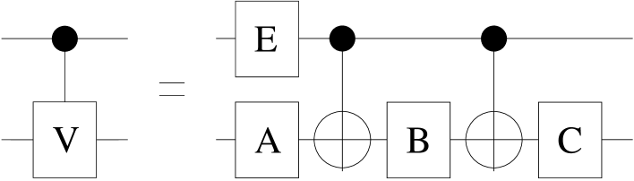
Here is a matrix such that . We further showed how these two-bit controlled-V gates could be further broken down, as shown in Fig. 8. Here , , , and are one bit gates for which we (Barenco et al. 1995) have obtained explicit formulas.
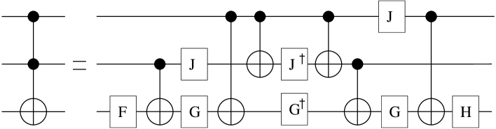
Thus, the circuit elements which would be needed in any quantum computation in which we are currently interested can be readily be simulated by short sequences of two-bit gates. For instance, the Toffoli gate, which would be the basis of much of the ordinary boolean logic which is needed for large sections of, for example, Shor prime factoring, can be obtained with just 6 XORs and 8 one-bit gates by using the constructions above; this is shown in Fig. 9. The unitary operators for the one-bit gates in this construction are
| (10) |
It may be noted that in this construction the gates can be grouped into a sequence of just five two-bit operations: first a 2-3 operation, then 1-3, 1-2, 2-3, and finally 1-3 (numbering the qubits 1-2-3 from the top). Numerical simulations (DiVincenzo & Smolin 1994; Smolin & DiVincenzo 1996) have indicated that the Toffoli gate can be obtained with no fewer than five two-bit quantum gates of any type.
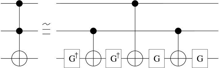
In a related result, Margolus has found (Barenco et al. 1995) an “almost” Toffoli gate which requires even less resources, as shown in Fig. 10: just three XORs and four one-bit gates (three two-bit gates overall). It is “almost” in the sense that one of the matrix elements of the Toffoli gate in Eq. (4) is changed from 1 to (the one corresponding to the state). This is not generally acceptable for quantum computation, where all the phases must be correct; however, we have noted (Barenco et al. 1995; Cleve & DiVincenzo 1996) that in many quantum programs the Toffoli gates appear in pairs, so that the “wrong” phase of the Margolus construction can be arranged to cancel out.
4 Gate constructions for quantum error correction
I wish to briefly touch upon a few points about the recent developments in error correction in quantum computation. Other authors in this book, and in many other papers, have given a very complete and rigorous discussion of this topic. Here I have only modest goals in mind: for the most part, I want to point out a few ways in which error correction uses and illuminates the ideas of quantum gate construction which I have been discussing above.

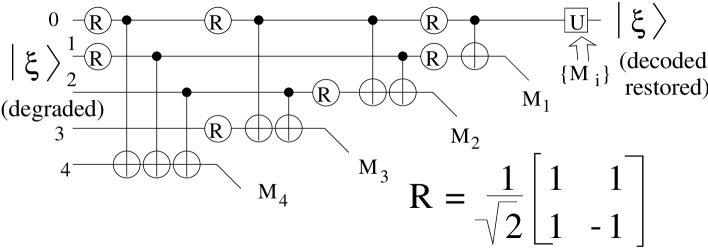
I begin immediately with a gate array shown in Fig. 11 which is of considerable interest to me (DiVincenzo & Shor 1996). This is one of the simplest “restoration” networks which works on a qubit state
| (11) |
where
and
Thus, is coded into this two-dimensional subspace of the five qubits entering the network from the left. The network operates in such a way that if has been degraded by noise, but only in such a way that no more than one of the five qubits is significantly damaged (a condition which is true at short times for most models of decoherence), then the network can restore the coded qubit exactly to its pristine state. We learned to our surprise from the work of Shor (Shor 1995) that this would be true independent of the state of the qubit in Eq. (11), that is, independent of the coefficients and ; thus we seemed to arrive at some sort of “analog” error correction, which had been believed to be impossible. Nevertheless, there is some deeper sense in which the error correction scheme which this network embodies is really more akin to that performed in digital computation. I will leave this thorny issue for other thinkers to try to articulate, but I hope to illustrate this by explaining how this error correction network manages to operate. At the level of the recipe needed to obtain this and similar networks, the procedure is very “digital.”
Now, to return to the main point, the essence of the error restoration of Fig. 11 is that it is performing four non-demolition measurements, the outcomes of which are labeled , , , and in the figure. If the one bit (Hadamard) rotations were absent, then the effect of each measurement is easily understood in classical Boolean logic (see Fig. 6). Then the effect of the XORs, say in , is to collect up the parity of the bits 0, 1, 2, and 4, saving this parity in the ancilla bit . Quantum mechanically, the parity of these qubits is given by the eigenvalue of the Hermitian operator , where the eigenvalue corresponds to even parity and the eigenvalue to odd parity. Indeed, the effect of the four XOR gates is exactly to perform the non-demolition measurement of this operator (see above for a discussion of simple non-demolition measurement by one XOR gate). The two gates preceding it can be thought of as basis changes for qubits 0 and 1. As it happens, this basis change is one which interchanges and labels, i.e., , , and . (Any sign changes in this basis transformation are irrelevant, since these operators are just specifying the basis of a measurement.) Thus, in Fig. 11 is actually a measurement of the operator on the state . The full set of four commuting operators which are measured (in non-demolition fashion) by this network are
| (14) |
As has been shown in the beautiful work on the theory of stabilizer-group codes by Gottesman (1996) and Calderbank et al. (1996), the outcomes of these four measurements can completely diagnose the error which has occurred on the coded quantum state (assuming that the error affects no more than one qubit), so that a final rotation (the gates of Fig. 11) of the qubits which have been determined to be in error will completely restore the coded state to its pristine form before decoherence.
Almost all the quantum codes which have been discovered up until now (the only exceptions that I know of are the single examples provided by Leung et al. (1997) and Rains et al. (1997)) are specified by generators like in Eq. (14), which are given as products of Pauli matrix operators. It is clear that the method exemplified in Fig. 6 for doing non-demolition measurements can be easily generalized to any product of Pauli-matrix operators. The rules can be summarized as follows: 1) make a basis change on each of the qubits so that the Pauli operator is changed to a . There are just two cases: If the operator is , then do the basis change with as above. If the operator is , then change basis with
| (15) |
Which produces the transformation , , , interchanging and as desired. 2) XOR each of the bits involved into an ancilla bit. Then a measurement of the ancilla bit is the desired non-demolition measurement. 3) In most cases it is desirable to undo the one-bit operations in order to restore the coded qubits to their original basis.
The above discussion of the “restoration” network is largely of the work reported in (DiVincenzo & Shor 1996). What has not been previously discussed is how a very similar procedure leads to a “decoding” network for the same quantum code. Decoding is like restoration in that non-demolition measurements are performed to determine the error syndrome. Unlike in restoration, the mapping takes the state from the coded form (or a noisy version thereof) to the “bare” form . Such decoding has been discussed by Cleve & Gottesman (1996), but the procedure which I will now describes seems to be a little more compact than theirs.
I will describe “decoding” by going through it for the same five bit code as above. The result is summarized in Fig. 12. I will proceed by keeping track of the evolution of the four operators describing the non-demolition measurement, Eq. (14), through the basis changes made in the course of the decoding. The first basis change has exactly the same purpose as in the restoration network, to bring the first operator into a form involving only ’s:
| (16) |
Now the next three XOR gates just accomplish a series of two-bit basis changes. The effect of these basis changes is easy to tabulate (Bennett et al. 1996; Calderbank et al. 1996):
| (17) |
These equations are true modulo , which, as explained above, are irrelevant for the error restoration or decoding. denotes the identity operator, and the subscripts and denote operators on the source and target bits. Using this table, the effect of the first three XOR gates in Fig. 12 may be easily worked out. The four operators become:
| (18) |
Note that the first operator can be measured by just making a conventional measurement on spin 4; and that is what is done. Of the other three operators, only the third operator also involves spin 4. Since all these operators commute, the dependence can only be ( and would anticommute). It is always possible to create new measurement operators by mutiplying two operators together (Calderbank et al. 1996), and if we do so here, the dependence on spin 4 is eliminated in the third operator. Because of the commuting condition, the spin-4 dependence can always be eliminated from all the measurement operators except one. Thus, after measurement of qubit 4, qubits 0-3 still remain, and it still remains to measure the operators
| (19) |
These can be dealt with in turn in exactly the same way. Choosing to simplify the last of these operators, the next set of one operation and two XORs lead to new operators
| (20) |
Now the second measurement becomes a measurement of the last remaining operator. Repeating this, the operators remaining to be measured are
| (21) |
Now we choose to simplify the first remaining operator with the next set of one operation and two XORs leading to the modified operators
| (22) |
Measuring qubit two gives the next bit of the syndrome. We finally have just one remaining operator to measure,
| (23) |
which is accomplished by the final two s and single XOR in the circuit. Finally, a one-bit rotation conditional on the measured syndrome bits is applied, just as in the restoration network of Fig. 11 (DiVincenzo & Shor 1996), to obtain the error corrected, “bare” qubit.
This procedure provides a much more systematic procedure for obtaining the restoration network than in the original work (Laflamme et al. 1996; Bennett et al. 1996), although it is not clear that the optimal network could be obtained by this procedure (Braunstein & Smolin 1997). The procedure given above requires gates, as in the decoding networks proposed by Cleve & Gottesman (1996); however, the present procedure is superior in that the decoding and the collection of the error syndrome are done simultaneously. It should also be noted that Fig. 12 can be converted directly into an encoding network by inversion, with the final operation removed and the measurements replaced by prepared states.
It is also worthwhile to recall that this network, applied bilaterally to both halves of five corrupted EPR pairs, results in the purification of these pairs (Bennett et al. 1996). The stabilizer-group theory which we use now shows us that it is unnecessary ever to use unilateral gate operations in the purification of Bell states, which was not clear in our original work. We see that each stage of non-demolition measurement illustrated above is equivalent to one step of what we referred to as “one-way hashing” in our original paper (Bennett et al. 1996). In our original language, each sequence of s and XORs accumulates a generalized parity bit of a subset of the amplitude and phase bits specifying the Bell states. For completeness, I note here, in the notation of the original paper, the “random” parity strings implemented in the network of Fig. 12:
| (24) |
Finally, I would like to say a few words about the relation between the non-demolition measurement operators appearing in the stabilizer code theory and the operators considered some seven years ago by Mermin (Mermin 1990) in his study of states which violate the Einstein-Podolsky-Rosen (EPR) notion of locality without the requirement of Bell inequalities. I leave most of this discussion to my paper with Asher Peres (DiVincenzo & Peres 1997) on this subject.
Mermin gave the simplest form of the states introduced by Greenberger, Horne and Zeilinger (see Zeilinger et al. 1997); one of the states he considered was
| (25) |
This is obviously a highly entangled state; it is also a kind of “code” state, in that you might view the 000 and 111 as being simple triple repetition codes standing for 0 and 1. The EPR paradox which was brought out by Mermin involve the following four operators:
| (26) |
The similarity with the measurement operators should already be evident. These are again a set of commuting operators involving the Pauli operators on the set of particles. Unlike in error correction, these operators are not all independent; the fourth one is the negative of the product of the first three. Of course, in the error correction scheme products of the measurement operators also produce valid syndrome measurements. The appearance of a redundant operator is actually quite crucial to the contradiction which Mermin draws, as I will explain in a moment. As in error correction, the four error operators are eigenoperators on the state ; so indeed is exactly like the protected subspace in the error correction scheme.
The current development of error correction has diverged from Mermin’s work in what one does with the set of operators. Rather than doing a non-demolition measurement of the whole set of operators, Mermin envisions a thought experiment in which a “demolishing” experiment is done of one of the four operators on each run of an experiment which begins with a perfect GHZ state. (No noise is considered in the Mermin setup.) In this “demolishing” experiment the three particles are imagined to be widely separated, and the operators are measured by measuring each of the one-particle measurements separately; this is followed by a classical comparison of the three measured results. GHZ were constructing cases in which one could contradict the assertion of “hidden variable” theories of quantum mechanics (the viewpoint of EPR) that the values of operators on one particle which can be determined by examination (i.e., measurement) of other, separated particles must constitute “elements of reality”, and thus have values which were preset at the time that the quantum state was prepared.
Mermin pointed out that this assertion is contradicted in his GHZ thought experiment. First, he notes that every Pauli operator on every particle conforms to the definition of an element of reality, and thus should have a preset value for the GHZ state. Then if he multiplies the preset values of the four operators in Eq. (26) the value must always be , since every operator appears exactly twice and each can only be preset to values . However, obviously the product of the actual four measurements from the discussion above is . This is the flat contradiction of hidden variables which Mermin pointed out.
We see from this example that much of the machinery of quantum error correction was actually latent in this previous work on the foundations of quantum mechanics; we (DiVincenzo & Peres 1997) have found that all the presently-proposed quantum error correcting codes provide exactly the same type of contradiction of hidden-variable theory as Mermin found for the GHZ state. This should not surprise us, given the close relation, as exemplified in much of the work at this conference, between quantum computation and the foundations of quantum theory. I expect that this association will continue to produce fruitful results in the future.
Acknowledgements.
I thank the other authors who collaborated with me on the work described here: A. Barenco, C. Bennett, R. Cleve, N. Margolus, A. Peres, P. Shor, T. Sleator, J. Smolin, H. Weinfurter and W. Wootters.References
- [1] Barenco, A., Bennett, C. H., Cleve, R., DiVincenzo, D. P., Margolus, N., Shor, P., Sleator, T., Smolin, J. A. & Weinfurter, H. 1995 Phys. Rev. A 52 3457-3467.
- [2] Baym, G. 1969 Lectures on Quantum Mechanics, pp. 140, 317-324. Benjamin-Cummings: Reading, Massachusetts.
- [3] Benioff, P. 1982 J. Stat. Phys. 29 515.
- [4] Bennett, C. H. 1973 IBM J. Res. Develop. 17, 525-532.
- [5] Bennett, C. H. 1989 SIAM J. Comput. 18 766.
- [6] Bennett, C. H., DiVincenzo, D. P., Smolin, J. A. & Wootters, W. 1996 Phys. Rev. A 54 3824-3851.
- [7] Braunstein, S. & Smolin, J. A. Phys. Rev. A 55 945-950; Report No. quant-ph/9604036.
- [8] Calderbank, A. R., Rains, E. M., Shor, P. W. & Sloane, N. J. A. 1996 Phys. Rev. Lett. 78, 405-408.
- [9] Chuang, I. L. & Yamamoto, Y. 1996 Phys. Rev. Lett. 76 4281-4284.
- [10] Cleve, R. & DiVincenzo, D. P. 1996 Phys. Rev. A 54 2636-2650.
- [11] Cleve, R. & Gottesman, D. 1997 Phys. Rev. A 55, in press (1 July); Report No. quant-ph/9607030.
- [12] DiVincenzo, D. P. 1995a Phys. Rev. A 51, 1015-1022.
- [13] DiVincenzo, D. P. 1995b Science 270, 255.
- [14] DiVincenzo, D. P. & Peres, A. 1997 Phys. Rev. A 55, in press (1 July); Report No. quant-ph/9611011.
- [15] DiVincenzo, D. P. & Shor, P. 1996 Phys. Rev. Lett. 77, 3260-3263.
- [16] DiVincenzo, D. P. & Smolin, J. 1994, in Proceedings of the Workshop on Physics and Computation, PhysComp ’94, p. 14, IEEE Computer Society Press: Los Alamitos, California.
- [17] Deutsch, D. 1985 Proc. R. Soc. London Ser. A 400 97.
- [18] Deutsch, D. 1989 Proc. R. Soc. London Ser. A 425 73.
- [19] Deutsch, D., Barenco, A. & Ekert, A. 1995 Proc. R. Soc. London Ser. A 449, 669.
- [20] Feynman, R. F. 1985 Opt. News 11 11.
- [21] Gottesman, D. 1996 Phys. Rev. A 54 1862.
- [22] Laflamme, R., Miquel, C., Paz, J.-P. & Zurek, W. H. 1996 Phys. Rev. Lett. 77 198-201.
- [23] Leung, D. W., Nielsen, M. A., Chuang, I. L. & Yamamoto, Y. 1997, Report No. quant-ph/9704002.
- [24] Levine, R. Y. & Sherman, A. T. 1990 SIAM J. Comput. 19, 673-677.
- [25] Lloyd, S. 1995 Phys. Rev. Lett. 75, 346-349.
- [26] Mermin, D. 1990 Physics Today 43 (no. 6), 9.
- [27] Monroe, C., Meekhof, D. M., King, B. E., Itano, W. M. & Wineland, D. J. 1995 Phys. Rev. Lett. 75 471-474.
- [28] Negele, J. W. & Orland, H. 1988 Quantum Many-Particle Systems, Eq. (2.11). Addison-Wesley: Reading, Massachusetts.
- [29] Rains, E. M., Hardin, R. H., Shor, P. W. & Sloane, N. J. A. 1997, Report No. quant-ph/9703002.
- [30] Shor, P. 1995 Phys. Rev. A 52 2493.
- [31] Sleator, T. & Weinfurter, H. 1995 Phys. Rev. Lett. 74, 4087-4090.
- [32] Smolin, J. & DiVincenzo, D. P. 1996 Phys. Rev. A 53 2855-2856.
- [33] Steane, A. M. 1996 Phys. Rev. Lett. 77 793-797.
- [34] Toffoli, T. 1980 in Automata, Languages and Programming, (eds. J. W. de Bakker and J. van Leeuwen), p. 632. Springer: New York.
- [35] Turchette, Q.A., Hood, C.J., Lange, W., Mabuchi, H. & Kimble, H.J. 1995 Phys. Rev. Lett. 75, 4710-4713.
- [36] Zeilinger, A., Horne, M. A., Weinfurter, H. & Zukowski M. 1997 Phys. Rev. Lett. 78 3031-3034.