[

Timing and Other Artifacts in EPR Experiments[1]

Abstract

Re-evaluation of the evidence (some of it unpublished) shows that experimenters conducting Einstein-Podolsky-Bohm (EPR) experiments may have been deceived by various pre-conceptions and artifacts. False or unproven assumptions were made regarding, in some cases, fair sampling, in others timing, accidental coincidences and enhancement. Realist possibilities, assuming a purely wave model of light, are presented heuristically, and suggestions given for fruitful lines of research. Quantum Mechanics (QM) can be proved false, but Bell tests have turned out to be unsuitable for the task.

]

Real EPR experiments are very different both from Einstein, Podolsky and Rosen’s original idea [3] and from Bell’s idealised situation [4]. The general scheme, which can have either one or two detection channels on each side, is described in a multitude of papers [5, 6]. Bell assumed no “missing values”, or, in other words, the certainty of detection in one channel or the other for all values of the “hidden variable”. As soon as real experiments were started, it was realised that detection would not be certain, and that consequently the inequalities would need to be modified. The result was a set of alternative inequalities [7] (see simplified versions, as generally used, in table I).

The standard inequality is covered in an earlier paper (“The Chaotic Ball: an Intuitive Analogy for EPR Experiments” [8]). Realist models that infringe it are easily constructed if (as I consider must always be the case) there are “variable detection probabilities”. The current paper presents likely explanations for (single-channel) experiments that infringe the CHSH or Freedman tests.

	Test Statistic	Upper Limit	Auxiliary
			Assumption
Standard	$S_{Std}=4(\frac{x-y}{x+y})$	2	Fair sampling
CHSH	$S_{C}=3\frac{x}{Z}-\frac{y}{Z}-2\frac{z}{Z}$	0	No enhancement
Freedman	$S_{F}=\frac{x-y}{Z}$	0.25	”

TABLE I.: Various Bell inequalities, for rotationally invariant, factorisable experiments. $x=R(\pi/8)$, $y=R(3\pi/8)$, $z=R(a,\infty)$ and $Z=R(\infty,\infty)$, using the usual terminology in which $R$ is coincidence rate, $a$ is polariser setting, and $\infty$ stands for absence of polariser.

Such experiments require more than simple variable probabilities, and very few experiments have, to my knowledge, achieved violation. These few are important, however, as they include the ones that have now gained a place in the text books, namely the single-channel Orsay experiments [9]. The assumptions behind the CHSH and Freedman inequalities are both the basic one of “factorability” (for each hidden variable value $\lambda$, the probability of a coincidence, $p_{c}(\lambda)=p_{1}(\lambda).p_{2}(\lambda)$, where $p_{1}(\lambda)$ and $p_{2}(\lambda)$ are the singles probabilities) and the additional one of “no enhancement” (for each $\lambda$ we have $p(a,\lambda)\leq p(\infty,\lambda)$).

Marshall, Santos and Pascazio [10, 11] have suggested that the latter assumption may be untrue, and this may well be the case [12]. They have also suggested that it could be the unjustifiable subtraction of “accidental coincidences” in some experiments that causes the violations, which would mean that we have both a kind of enhancement and a failure of factorability, but caused by erroneous manipulation of the data rather than any fundamental property of the experimental setup. Though Aspect and Grangier[13] have countered their criticisms, there remain severe doubts: the figures they quote are for the two-channel experiment [14], which uses the standard test.

	$x$	$y$	$z$	$Z$	$S_{Std}$	$S_{C}$	$S_{F}$
Raw coincidences	86.8	38.3	126.0	248.2	1.55	-0.121	0.195
Accidentals	22.8	22.5	45.5	90.0
“Corrected”	64.0	15.8	80.5	158.2	2.42	0.096	0.309

TABLE II.: Effect of standard adjustment for accidental coincidences. Data from table VII-A-1 of Aspect’s thesis (1981 single-channel experiment).

My own figures (table II), extracting relevant information from Aspect’s thesis [15], suggest that no Bell test for single-channel experiments would have been violated had “accidentals” not been subtracted.

The mechanism whereby accidentals can cause violation is very straightforward. We can be fairly confident that Bell’s inequalities will hold for the raw data, but whether or not they hold after subtraction depends on whether or not true and accidental detections are independent. This depends on factors such as correlations between neighbouring emissions, how the detector responds to close (actually overlapping, under a wave model) signals and instrument dead times. The number of accidentals (as measured by the number of coincidences when one stream is delayed by, say, 100 ns) is proportional to the product of the numbers of signals on each side. If the detectors are “correctly” adjusted, so that they register half the number of hits when a polariser is inserted (which follows from Malus’ Law provided noise and settings of various voltages are appropriate [16]), the value is $A$, say, for terms such as $x$ and $y$, $2A$ for terms $z$, and $4A$ for terms $Z$. It is easily seen that if we subtract these we increase all test statistics and hence the likelihood of violations.

Let us review the situation, as the question of accidentals is inextricably entangled with the whole matter of timing, choice of coincidence window and the interpretation of time spectra.

FIG. 1.: Assumed ideal timing and resultant spectrum. $D$ is the delay applied to the $B$ channel so as to place the peak in the centre of the picture.

Proofs of Bell inequalities do not mention time. They assume that the source produces pairs of particles and that identification of the pairs poses no problem. Thus the stream of signals arriving at the coincidence monitor (the device which in practice does the identification) can be envisaged as in Fig. 1, which also shows the expected time-spectrum — a single bar whose height is the number of coincidences. Even this simple picture might have a slight complication, as the pairs are supposed to be produced at completely random times. This means that there is a very slight possibility that there will be another $B$ arrival at any interval after the $A$ (including in the same “time-bin”), so that we expect a low constant background of accidentals, or rather, because the instrument measures the time to the first detection, a downward slope that is gentle provided the emission rate is low or the probability of detection is small.

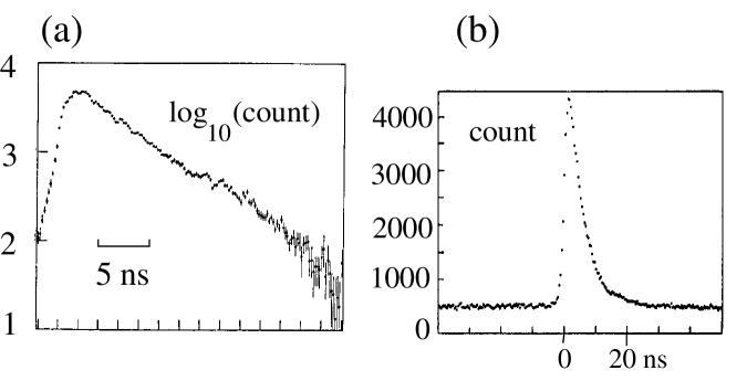
FIG. 2.: Actual time spectra. (a) Freedman, (b) Aspect. Freedman’s could have been slightly distorted by the instrumentation. It is drawn by hand and represents the combined results of a whole series of runs. Aspect’s is for just one run and would have been displayed on a VDU (actual runs would have had considerably greater scatter as they were over shorter periods)

Consider now some spectra (histograms of differences in detection times of $A$ and $B$ signals) from actual experiments, Freedman’s of 1972 [17] and Aspect’s of around 1980 (Fig. 2). Numbers of coincidences can be estimated by defining an “integration window” and organising electronics so as to count all signals that arrive within it. It is conventionally described in terms of just the one parameter, $w$, though in reality it requires two — a start time relative to the peak of the spectrum, as well as the window length. Aspect in his final experiment used a window from $-3$ ns to $+17$ ns. Freedman used one of just 8 ns length, but does not tell us how the start was chosen. Note that the difference in shape between the two spectra is due primarily to the scales — log in one case, not in the other.

From their PhD theses, it is clear how the experimenters were interpreting their time-spectra. Both Aspect and Freedman were thinking of the decreasing region as showing the distribution of emission times (controlled by the “lifetime of the intermediate stage of the cascade”) of the second “photon”, this being regarded as a particle. They took the rising front as due to random, normally distributed, timing variations. There was a constant underlying background of accidentals.

Now under a classical wave theory of light, this interpretation is not reasonable on several counts. Firstly, various considerations (see above) make the assumption of constant accidentals implausible. Secondly, if the rise were due just to random variations, then would not the peaks of the spectra be broader? (Interestingly, Aspect mentions that the variations do cause a broadening, but this is not evident here.) Under wave theory, the results seem to indicate rather that the $A$ and $B$ “photons” are emitted simultaneously, and each is a wave that starts at high intensity and decreases at roughly negative exponential rate, only the $A$ one much more fast than the $B$. (We assume that detection occurs when the addition of electromagnetic noise to the signal pushes the total over some threshold.) This interpretation becomes more obvious if one thinks of the pairs of equal “photons” of the Stirling experiments [18], in which the time-spectra are symmetrical. There is possible experimental support for this view: it might explain Aspect’s problems with “post-impulsions”, or multiple detections, some of which occurred despite dead times of 16 ns or more.

If we admit, however, that the rising front is not solely the result of random time variations — and they are, in any case, most unlikely to be normally distributed — this raises the question of how we interpret the various observed timing variations. They are only small (standard errors of about 0.7 ns for each photomultiplier and 0.1 ns for each discriminator, according to Aspect’s investigations [15], but if they were systematically related to the polarisation angles — which they would be if related to intensity of the input [19] — then they could contribute to a systematic change in the quality of synchronisation between different values of $\phi$, the angle between polariser settings. This could, if windows were too small to include all genuine coincidences, mean that factorability did not hold exactly [20]. It could mean that $R(\pi/8)$, involving the smaller angle, was based on pairs that were slightly better synchronised than $R(3\pi/8)$, giving a slight increase to the difference and hence a slight increase in the chance of violating a Bell inequality.

Aspect was aware of the need to ensure that his window included all true coincidences. His theoretical calculations suggested that he included 97% of them, but he never mentions the danger of systematic time variations, which could mean slight differences in shape between spectra for different $\phi$. He would not have been able to detect such differences by eye, due to scatter and accidentals, and it is impossible to tell whether or not his chosen window was adequate. Freedman’s was too small unless accepted theory is absolutely perfect. Both Aspect and Freedman used as their main criterion the maximisation of a “quality factor”. This amounted to minimising the running time of the experiment — surely of lesser importance than the avoidance of systematic error?

A slight timing effect may well be present in all cascade experiments, but is unlikely to be the prime cause of inequality violations. As mentioned above, it is more likely in Aspect’s experiments that the accidental coincidence subtraction is the prime cause, and if we think again about Freedman’s spectrum (Fig. 2 (a)), we might suspect from what he tells us of the conditions under which it was obtained that there is a rather more crude effect coming into play here. It could be simply a matter of presence or absence of the polarisers producing small changes in transit times, shifting the whole spectrum. The polarisers were very large (“pile of plates” type, 180 cm long), so, though the thickness of the glass in them was small, if there were multiple reflections a nanosecond or so of variation might occur. Poor choice of start and end of his very short window could then easily cause bias towards lower values with polariser absent, which could lead to inequality violation. Aspect, it should be noted, “corrected” for any such effect by adjusting a variable delay.

This has brought us a long way from Bell’s simple idea, and the limits of complexity of the real situations have only just started to be explored. Much more could be said about the effect of our assumptions about the emission process (Is it really random, or is there any slight tendency to clustering, or, conversely, to even spacing in time?); about the effects of dead times (various different ones come into play at different points in the experiments, having the effect of (a) suppressing multiple detections and (b) adding yet one more difference between the sets of signals that constitute “singles” and the “coincidences”); and about the detection process (Is it necessarily “square law” for the full range of signals encountered? Is the electromagnetic noise that is an essential part of the process [21] steady or does it fluctuate?).

My own interest has been in exploring the possibility that time spectra may have extended tails when produced by attenuated signals. These tails would arise if the signals were in fact decaying only very slowly and the probability of detection per unit time were high. (It would be sufficient to have the probability high for some subset of the whole set of signals.) The effect arises because the time spectrum shows the time to the first detection only, so that the probability for a given time-delay may be greater if the probability that the current signal was not detected prior to this is smaller. The fascination of this subject was the possibility of a completely different demonstration of the pure wave nature of light, in the time-domain instead of the familiar spatial domain of the two-slit experiment. It is interesting that experimenters assume that measuring an atomic lifetime using time-spectra (which measure the first detection times) is exactly equivalent to a method in which many “photons” are detected simultaneously and produce directly a time-varying electric signal. A paper detailing the method is quoted by Aspect as an authority on measurement of lifetimes [22]. Computer simulations have shown that experiments to date have probably not been suitable for showing this effect, but it might be possible to devise one, with very low emission rate or with the more controllable pairs of signals produced in parametric down-conversion.

To return to matters of more immediate importance, Aspect’s experiments involved seriously large accidental coincidences. As he says, there could typically be 600 accidentals to 200 true coincidences displayed on the VDU. One can seriously question, therefore, whether it is possible to extract a valid Bell-type test from such data. His idealisation is illustrated by Fig. 3(a), taken from his thesis. But we have no independent way of judging the true picture. This (if one can be said to exist) might be as in Fig. 3(b).

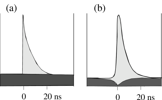
FIG. 3.: Models of time spectra: (a) quantum mechanics assumption and (b) conjectural realistic model. Light shading: “true”; Dark shading: “accidental” coincidences.

Freedman’s experiment is perhaps the only one to have been performed in which accidentals do not appear to be important — we get violation of inequalities even when they are not subtracted — but, as explained above, it used a coincidence window that was too small. It was wide open to synchronisation problems.

There appears to have been a serious miscarriage of science in accepting existing experiments as supporting quantum theory. Logically, this hypothesis should have been rejected at the outset, as the implied non-local effects are impossible. It is evident that existing classical explanations are also wrong, as they give wrong predictions. It should therefore have been realised that all existing theory should have been challenged. It should not have been possible for Aspect to make statements such as (translating loosely from his thesis): “Agreement with quantum theory is a privileged method for confirming that the apparatus is correctly set” (referring, presumably, not to the final conclusion of Bell violations but to intermediate decisions such as conformity to Malus’ Law). Freedman concluded his thesis with a remark to the effect that there was no need to search too hard for causes of systematic error as Bell’s inequalities had been violated and were of such general applicability. Many workers have allowed themselves to be influenced by an opinion that any imperfections would bring quantum theory predictions nearer to classical ones. Perversely, this has turned out to be true, but it is the classical ones that are brought nearer to quantum theory, not the other way around!

To conclude, I should like to take this opportunity to state some general opinions. Firstly, the setup of EPR experiments could be put to much more constructive use than merely attempting violate Bell inequalities. By exploring objectively a wider range of parameters, with detectors purposely set “wrongly” (so that we do not get Malus’ Law reproduced or neat results such as doubling coincidences when we remove a polariser), these experiments could prove that light is purely wave — that it is not a matter of the polariser passing a certain percentage of “photons” but of it reducing the intensity of each signal, in exactly the same way as on a classical level though (see Marshall and Santos’s Stochastic Optics work) being subject, due to the very low intensities, to random variations from additions of background electromagnetic noise. Secondly, I would suggest that computer simulations should be conducted in parallel with the experiments. The act of constructing the computer model brings home the logical structure, which cannot possibly be that of the Quantum Mechanics collapsing wavefunction. This, as Feynman showed [23], cannot be simulated.

REFERENCES

- [1] Submitted to Physical Review Letters, April 24, 1997.
- [2] Electronic address: cat@aber.ac.uk
- [3] A. Einstein, B. Podolsky, and N. Rosen, Physical Review 47, 777 (1935).
- [4] J. S. Bell, Physics 1, 195 (1964).
- [5] F. Clauser, John and A. Shimony, Reports on Progress in Physics 41, 1881 (1978).
- [6] F. Selleri, Quantum Mechanics Versus Local Realism: The Einstein-Podolsky-Rosen Paradox (Plenum Press, New York, 1988).
- [7] J. F. Clauser and M. A. Horne, Physical Review D 10, 526 (1974).
- [8] C. H. Thompson, Foundations of Physics Letters 9, 357 (1996). (Available electronically at http://xxx.lanl.gov, ref quant-ph/9611037.)
- [9] A. Aspect, P. Grangier, and G. Roger, Physical Review Letters 47, 460 (1981); A. Aspect, J. Dalibard, and G. Roger, Physical Review Letters 49, 1804 (1982).
- [10] E. Santos, in Open Questions in Quantum Physics, Tarozzi and van der Merwe eds., D. Reidel Pub. Co. Dordrecht 291 (1985); T. W. Marshall and E. Santos, Physics Letters A 107, 164 (1985).
- [11] S. Pascazio, in The Concept of Probability, E. I. Bitsakis and C. A. Nicolaides (eds.): Kluwer Academic Press 105 (1989).
- [12] Gilbert and Sulcs (private communication) have pointed out that enhancement can be regarded as an established fact, showing, for example, in an increase in intensity when a scatterer is placed between two polarising sheets.
- [13] A. Aspect and P. Grangier, Lettere al Nuovo Cimento 43, 345 (1985).
- [14] A. Aspect, P. Grangier, and G. Roger, Physical Review Letters 49, 91 (1982).
- [15] A. Aspect, Trois tests expérimentaux des inégalités de Bell par mesure de corrélation de polarisation de photons (PhD thesis No. 2674, Université de Paris-Sud, Centre D’Orsay, 1983).
- [16] Malus’ Law should not be assumed in EPR experiments. It may well be that it holds exactly for intensities, but a realist theory of detection must admit the likelihood that the probability of detection is not exactly proportional to the intensity. Hence Malus’ Law would not in general hold exactly for the measured counts.
- [17] S. J. Freedman, Experimental test of local hidden-variable theories (PhD thesis (available on microfiche), University of California, Berkeley, 1972).
- [18] W. Perrie, A. J. Duncan, H. J. Beyer, and H. Kleinpoppen, Physical Review Letters 54, 1790 (1985).
- [19] The received wisdom has been, since Lawrence and Beams’ work in the 1920s, that timing does not vary with intensity. Most likely the minimum time does not vary, but I suggest that mean and spread are highly likely to.
- [20] A. Fine, Physical Review Letters 48, 291 (1982); S. Pascazio, Physics Letters A 118, 47 (1986).
- [21] B. C. Gilbert and S. Sulcs, Foundations of Physics 26, 1401 (1996).
- [22] M. D. Havey, L. C. Balling, and J. J. Wright, Journal of the Optical Society of America 67, 488 (1977).
- [23] R. P. Feynman, International Journal of Theoretical Physics 21, 467 (1982).