Added noise in homodyne measurement of field-observables

Abstract

Homodyne tomography provides a way for measuring generic field-operators. Here we analyze the determination of the most relevant quantities: intensity, field, amplitude and phase. We show that tomographic measurements are affected by additional noise in comparison with the direct detection of each observable by itself. The case of of coherent states has been analyzed in details and earlier estimations of tomographic precision are critically discussed.

1 Introduction

One of the most exciting developments in the recent history of quantum optics is represented by the so-called Homodyne Tomography, namely the homodyne detection of a nearly single-mode radiation field while scanning the phase of the local oscillator [1, 2, 3, 4]. ¿From a tomographic data record, in fact, the density matrix elements can be recovered, thus leading to a complete characterization of the quantum state of the field. This is true also when not fully efficient photodetectors are involved in the measurement, provided that quantum efficiency is larger than the threshold value $\eta=1/2$.

In homodyne tomography a general matrix element is obtained as an expectation value over homodyne outcomes at different phases. In formula

$$\langle\psi|\hat{\varrho}|\varphi\rangle=\int^{\pi}_{0}\frac{d\phi}{\pi}\int^{+\infty}_{-\infty}\!\!dx\>p_{\eta}(x;\phi)\>\langle\psi|K_{\eta}(x-\hat{x}_{\phi})|\varphi\rangle\,,$$ (1)

where $p_{\eta}(x;\phi)$ is the probability density of the homodyne outcome $x$ at phase $\phi$ for quantum efficiency $\eta$ and the integral kernel is given by

$$K_{\eta}(x)=\frac{1}{2}\hbox{Re}\int^{+\infty}_{0}\!\!dk\,k\,\exp\left(\frac{1-\eta}{8\eta}k^{2}+ikx\right)\,.$$ (2)

While the kernel in Eq. (2) is not even a tempered distribution, its matrix elements can be bounded functions depending on the value of $\eta$. This is the case of the number representation of the density matrix, for which the ”pattern function”

$$f_{n,n+d}^{(\eta)}(x,\phi)\equiv\langle n|K_{\eta}(x-\hat{x}_{\phi})|n+d\rangle\;.$$ (3)

can be expressed as a finite linear combination of parabolic cylinder functions [3].

As it comes from the experimental average

$$\overline{\varrho_{n,m}}=\int^{\pi}_{0}\frac{d\phi}{\pi}\int^{+\infty}_{-\infty}\!\!dx\,p_{\eta}(x;\phi)\>f_{n,n+d}^{(\eta)}(x,\phi)\,,$$ (4)

the tomographic determination $\overline{\varrho_{n,m}}$ for the matrix element $\varrho_{n,m}\equiv\langle n|\hat{\varrho}|m\rangle$ is meaningful only when its confidence interval is specified. This is defined, according to the central limit theorem, as the rms value rescaled by the number $N$ of data. As $\varrho_{n,m}$ is a complex number, we need to specify two errors, one for the real part and one for the imaginary part respectively. For the real part one has

$$\hbox{Re}\>\varepsilon_{n,m}=\frac{\overline{\Delta\hbox{Re}\varrho_{n,m}}}{N}=\frac{\left\{\overline{\hbox{Re}\varrho^{2}_{n,m}}-\left[\hbox{Re}\overline{\varrho_{n,m}}\right]^{2}\right\}^{1/2}}{N}\,,$$ (5)

where

$$\overline{\hbox{Re}\varrho^{2}_{n,m}}=\int^{\pi}_{0}\frac{d\phi}{\pi}\int^{+\infty}_{-\infty}\!\!dx\,p_{\eta}(x;\phi)\>\left[\hbox{Re}f_{n,n+d}^{(\eta)}(x,\phi)\right]^{2}\>,$$ (6)

and likewise for the imaginary part.
Quantum tomography opened a fascinating perspective: in fact, there is the possibility of device-independent measurements of any field-operator, including the case of generalized observables that do not correspond to selfadjoint operators as, for example, the complex field amplitude and the phase. The first application in this direction has been presented in Ref. [5] where the number and the phase distributions of a low excited coherent state have been recovered from the original tomographic data record. No error estimation was reported in Ref. [5], whereas an earlier analysis of the precision of such determinations has been reported in Ref. [6] on the basis of numerical simulations. The idea behind these papers is simple. Any field operator $\hat{A}$, in fact, is described by its matrix elements $A_{n,m}\equiv\langle n|\hat{A}|m\rangle$ in the number representation. Then, upon a suitable truncation of the Hilbert space dimension, at the maximum photon number $H$, the expectation value of $\hat{A}$ is given by the linear combination

$$\langle\hat{A}\rangle=\sum_{n,m=0}^{H}\overline{\varrho_{n,m}}\ A_{n,m}\>,$$ (7)

whereas the corresponding confidence interval is evaluated by error propagation calculus

$$\overline{\Delta A}^{2}\simeq\sum_{n,m=0}^{H}\left|\overline{\Delta\varrho_{n,m}}\right|^{2}\>\left|A_{n,m}\right|^{2}\,.$$ (8)

The whole procedure relies on two assumption, namely

$$\varrho_{n,m}\ll 1\qquad n,m>H\,,$$ (9)

and

$$\lim_{n,m\rightarrow\infty}\overline{\Delta\varrho_{n,m}}=0\,,$$ (10)

which needs a more careful analysis. The condition in Eq. (9) is certainly fulfilled for some value of $H$, whose determination, however, requires an a priori knowledge of the state under examination. On the other hand, it has been shown in Ref. [7] that in a tomographic measurement involving $N$ experimental data the errors $\hbox{Re}\>\varepsilon_{n,m}$ and $\hbox{Im}\>\varepsilon_{n,m}$ saturate to the value $\sqrt{2/N}$ for $\eta=1$, whereas they diverge exponentially for $\eta<1$. Therefore, the condition (10) cannot be fulfilled in a real experiment and we conclude that determinations of Ref. [5] are not meaningful, as they are affected by diverging errors and are based on a priori knowledge of the state. For the same reason the analysis of Ref. [6] is not correct, and the added noise has been largely overestimated.

2 Homodyning field operators

In this paper we analyze the tomographic determination of field-quantities from a different perspective. By homodyning an observable $\hat{A}$ we mean the average

$$\langle\hat{A}\rangle=\int^{\pi}_{0}\frac{d\phi}{\pi}\int^{+\infty}_{-\infty}\!\!dx\,p(x;\phi)\>{\cal R}[\hat{A}](x;\phi)\,,$$ (11)

of the state-independent kernel function ${\cal R}[\hat{A}](x;\phi)$ [8], which allows for the determination of the expectation value $\langle\hat{A}\rangle$ without the detour into density matrix elements. For a Hilbert-Schmidt operator $\hat{A}$ Eq.(11) follows directly from a generalization of Eq.(1) with ${\cal R}[\hat{A}](x;\phi)=\hbox{\rm Tr}\left\{\hat{A}K(x-\hat{x}_{\phi})\right\}$, whereas alternative approaches to derive explicit expressions of the kernel have been suggested [10, 8], that here we briefly recall. Starting from the identity involving trilinear products of Hermite polynomials (valid for $k+m+n=2s$ even [9] )

$$\int^{+\infty}_{-\infty}\!\!dxe^{-x^{2}}H_{k}(x)\,H_{m}(x)\,H_{n}(x)=\frac{2^{\frac{m+n+k}{2}}\pi^{{1\over 2}}k!m!n!}{(s-k)!(s-m)!(s-n)!}\;,$$ (12)

Richter proved the following nontrivial formula for the expectation value of the normally ordered field operators [10]

$$\langle a^{{\dagger}}{}^{n}a^{m}\rangle=\int^{\pi}_{0}\frac{d\phi}{\pi}\int^{+\infty}_{-\infty}\!\!dx\,p(x;\phi)e^{i(m-n)\phi}\frac{H_{n+m}(\sqrt{2}x)}{\sqrt{2^{n+m}}{{n+m}\choose n}}\;,$$

which corresponds to the kernel

$${\cal R}[a^{{\dagger}}{}^{n}a^{m}](x;\phi)=e^{i(m-n)\phi}\frac{H_{n+m}(\sqrt{2}x)}{\sqrt{2^{n+m}}{{n+m}\choose n}}\;.$$ (13)

For nonunit quantum efficiency the homodyne photocurrent is rescaled by $\eta$ whereas the normally ordered expectation $\langle a^{{\dagger}}{}^{n}a^{m}\rangle$ gets an extra factor $\eta^{{1\over 2}(n+m)}$. Therefore, one has

$${\cal R}_{\eta}[a^{{\dagger}}{}^{n}a^{m}](x;\phi)=e^{i(m-n)\phi}\frac{H_{n+m}(\sqrt{2\eta}x)}{\sqrt{(2\eta)^{n+m}}{{n+m}\choose n}}\;,$$ (14)

where the kernel ${\cal R}_{\eta}[\hat{O}](x;\phi)$ is defined as in Eq. (11), but now with the experimental probability distribution $p_{\eta}(x;\phi)$ for nonunit quantum efficiency $\eta$. From Eq. (14) by linearity one can obtain the kernel ${\cal R}_{\eta}[\hat{f}](x;\phi)$ for any operator function $\hat{f}$ that admits a normal ordered expansion

$$\hat{f}\equiv f(a,a^{{\dagger}})=\sum_{nm=0}^{\infty}f^{(n)}_{nm}a^{{\dagger}}{}^{n}a^{m}\;.$$ (15)

One obtains

$${\cal R}_{\eta}[\hat{f}](x;\phi) = \sum_{s=0}^{\infty}\frac{H_{s}(\sqrt{2\eta}x)}{s!(2\eta)^{s/2}}\sum_{nm=0}^{\infty}f^{(n)}_{nm}e^{i(m-n)\phi}n!m!\delta_{n+m,s}$$ (16)

$$= \sum_{s=0}^{\infty}\frac{H_{s}(\sqrt{2\eta}x)i^{s}}{s!(2\eta)^{s/2}}\frac{d^{s}}{dv^{s}}\Bigg{|}_{v=0}\!\!\!\!{\cal F}[\hat{f}](v;\phi),$$

where

$${\cal F}[\hat{f}](v;\phi)=\sum_{nm=0}^{\infty}f^{(n)}_{nm}{{n+m}\choose m}^{-1}(-iv)^{n+m}e^{i(m-n)\phi}\;.$$ (17)

Continuing from Eq. (16) one obtains

$${\cal R}_{\eta}[\hat{f}](x;\phi)=\exp\left(\frac{1}{2\eta}\frac{d^{2}}{dv^{2}}+2ix\frac{d}{dv}\right)\Bigg{|}_{v=0}{\cal F}[\hat{f}](v;\phi)\;,$$ (18)

and finally

$${\cal R}_{\eta}[\hat{f}](x;\phi)=\int_{-\infty}^{+\infty}\frac{dw}{\sqrt{2\pi\eta^{-1}}}e^{-\frac{\eta}{2}w^{2}}{\cal F}[\hat{f}](w+2ix;\phi)\;.$$ (19)

In summary, the operator $\hat{f}$ possesses a tomographic kernel ${\cal R}_{\eta}[\hat{f}](x;\phi)$ if the function ${\cal F}[\hat{f}](v;\phi)$ in Eq. (17) grows slower than $\exp(-\eta v^{2}/2)$ for $v\to\infty$. In addition, as we can assume that $p_{\eta}(x;\phi)$ goes to zero faster than exponentially at $x\to\infty$, the average in Eq. (11) is meaningful for the integral in Eq. (19) growing at most exponentially for $x\to\infty$. In the next section we will consider the tomographic determination of four relevant field quantities: the field intensity, the real field or quadrature, the complex field, and the phase, for all of which the above conditions are satisfied.

3 Added noise in tomographic measurements

As already mentioned in the previous section the tomographic measurement of the quantity $\hat{A}$ is defined as the average $\overline{w_{\eta}}$ of the kernel $w_{\eta}\equiv{\cal R}_{\eta}[\hat{A}](x,\phi)$ over the homodyne data. A convenient measure for the precision of the measurement is given by the confidence interval $\overline{\Delta w_{\eta}}$ which, being $w_{\eta}$ a real quantity, is given by $\overline{\Delta w_{\eta}}=\left\{\overline{w^{2}_{\eta}}-\overline{w_{\eta}}^{2}\right\}^{1/2}$, where

$$\overline{w^{2}_{\eta}}\equiv\overline{{\cal R}_{\eta}^{2}[\hat{A}](x,\phi)}=\int^{\pi}_{0}\frac{d\phi}{\pi}\int_{-\infty}^{\infty}\!\!dx\>p_{\eta}(x,\phi)\>{\cal R}^{2}_{\eta}[\hat{A}](x,\phi)\>.$$ (20)

When the quantity $\hat{A}$ can also be directly measured by a specific setup it makes sense to compare tomographic precision $\overline{\Delta w}$ with the corresponding fluctuations $\sqrt{\langle\widehat{\Delta A^{2}}\rangle}$. Notice that, when we deal with $\eta<1$ the noise $\sqrt{\langle\widehat{\Delta A^{2}}\rangle_{\eta}}$ is larger that the quantum fluctuations due to smearing effect of nonunit quantum efficiency. As we will see, the tomographic measurement is always more noisy than the corresponding direct measurement for any observable, and any quantum efficiency $\eta$. However, this is not surprising, in view of the larger amount of information retrieved in the tomographic measurement compared to the direct measurement of a single quantity.
In Table 1 we report the tomographic quantities $w_{\eta}$ the field-observables examined. Before going into details of each observable, we mention a useful formula for evaluating confidence intervals. These are obtained by averaging quantities like

$${\cal R}_{\eta}^{2}[a^{{\dagger}n}a^{m}](x,\phi)=e^{2i\phi(m-n)}\frac{H^{2}_{n+m}\left(\sqrt{2\eta}x\right)}{(2\eta)^{(n+m)}\left(\begin{array}[]{c}m+n\\ m\end{array}\right)^{2}}\>.$$ (23)

By means of the following identity for the Hermite polynomials [11]

$$H^{2}_{n}(x)=2^{n}n!^{2}\sum_{k=0}^{n}\frac{H_{2k}(x)}{k!^{2}\>2^{k}\>(n-k)!}\>,$$ (24)

we arrive at

$${\cal R}^{2}_{\eta}[a^{{\dagger}n}a^{m}](x,\phi)=e^{2i\phi(m-n)}\frac{n!^{2}m!^{2}}{\eta^{m+n}}\sum_{k=0}^{m+n}\frac{(2k)!\eta^{k}}{k!^{4}(n+m-k)!}{\cal R}_{\eta}[a^{{\dagger}k}a^{k}](x,\phi)\>,$$ (25)

which expresses the generic square kernel ${\cal R}^{2}_{\eta}[a^{{\dagger}n}a^{m}](x,\phi)$ in terms of ”diagonal” kernels ${\cal R}_{\eta}[a^{{\dagger}k}a^{k}](x,\phi)$ only.

3.1 Field-Intensity

Photodetection is the direct measurement of the field-intensity. For a single-mode of the radiation field it corresponds to the number operator $\hat{n}=a^{{\dagger}}a$. For nonunit quantum efficiency $\eta$ at the photodetectors, only a fraction of the incoming photons is revealed, and the probability of detecting $m$ photons is given by the Bernoulli convolution

$$p_{\eta}(m)=\sum_{n=m}^{\infty}\rho_{nn}\left(\begin{array}[]{c}n\\ m\end{array}\right)\eta^{m}(1-\eta)^{n-m}\>,$$ (28)

$\rho_{nn}$ being the actual photon number distribution of the mode under examination. One considers the reduced photocurrent

$$\hat{I}_{\eta}=\frac{1}{\eta}a^{{\dagger}}a\>,$$ (29)

which is the quantity that traces the photon number, namely it has the same mean value

$$\langle\hat{I}_{\eta}\rangle=\frac{1}{\eta}\sum_{m=0}^{\infty}m\>p(m)=\bar{n}\>,$$ (30)

where we introduced the shorthand notation $\bar{n}=\langle a^{{\dagger}}a\rangle$. On the other hand, one has

$$\langle\widehat{\Delta I^{2}}\rangle_{\eta}=\frac{1}{\eta^{2}}\sum_{m=0}^{\infty}m^{2}p(m)=\langle\widehat{\Delta n^{2}}\rangle+\bar{n}\left(\frac{1}{\eta}-1\right)\>.$$ (31)

In Eq. (31) $\langle\widehat{\Delta n^{2}}\rangle$ denotes the intrinsic photon number variance . The term $\bar{n}(\eta^{-1}-1)$ represents the noise introduced by inefficient detection. The tomographic kernel that traces the photon number is given by the phase-independent function $w_{\eta}\equiv 2x^{2}-(2\eta)^{-1}$. With the help of Eq. (25) we can easily evaluate its variance, namely

$$\overline{\Delta w_{\eta}}^{2}=\langle\widehat{\Delta n^{2}}\rangle+\frac{1}{2}\langle\widehat{n^{2}}\rangle+\bar{n}\left(\frac{2}{\eta}-\frac{3}{2}\right)+\frac{1}{2\eta^{2}}\>.$$ (32)

The difference between $\overline{\Delta w_{\eta}}^{2}$ and $\langle\widehat{\Delta I^{2}}\rangle_{\eta}$ defines the noise $N[\hat{n}]$ added by tomographic method in the determination of the field intensity

$$N[\hat{n}]=\frac{1}{2}\left[\langle\widehat{n^{2}}\rangle+\bar{n}\left(\frac{2}{\eta}-1\right)+\frac{1}{\eta^{2}}\right]\>.$$ (33)

The noise $N[\hat{n}]$ added by the tomographic measurement is always a positive quantity and largely depends on state under examinations. For coherent states we consider the noise-ratio

$$\delta n_{\eta}=\sqrt{\frac{\overline{\Delta w_{\eta}}^{2}}{\langle\widehat{\Delta I^{2}}\rangle_{\eta}}}=\left\{2+\frac{1}{2}\left(\eta\bar{n}+\frac{1}{\eta\bar{n}}\right)\right\}^{1/2}\;,$$ (34)

which is minimum for $\bar{n}=\eta^{-1}$.

3.2 Real Field

For a single mode light-beam the electric field is proportional to a field quadrature $\hat{x}=1/2(a^{{\dagger}}+a)$, which is just traced by homodyne detection at fixed zero-phase with respect to the local oscillator. The tomographic kernel, that traces the mean value $\hbox{Tr}\{\hat{\varrho}\hat{x}\}$ is given by $w_{\eta}\equiv{\cal R}_{\eta}[\hat{x}](x,\phi)=2x\cos\phi$, independently on $\eta$, whereas the square kernel $w_{\eta}^{2}\equiv{\cal R}^{2}[\hat{x}](x,\phi)=4x^{2}\cos^{2}\phi$ can be rewritten as

$$w_{\eta}^{2}=\frac{1}{4}\left[{\cal R}[a^{2}](x,\phi)+{\cal R}[a^{{\dagger}2}](x,\phi)\right]+{\cal R}[a^{{\dagger}}a](x,\phi)+\frac{1}{2\eta}\;.$$ (35)

The confidence interval is thus given by

$$\overline{\Delta w_{\eta}}^{2}=\frac{1}{4}\left[\langle a^{{\dagger}2}\rangle+\langle a^{2}\rangle\right]+\bar{n}+\frac{1}{2\eta}-\left\langle\frac{a+a^{{\dagger}}}{2}\right\rangle^{2}=\langle\widehat{\Delta x^{2}}\rangle+\frac{1}{2}\bar{n}+\frac{2-\eta}{4\eta}\;,$$ (36)

$\langle\widehat{\Delta x^{2}}\rangle$ being the intrinsic quadrature fluctuations. For coherent states Eq. (36) reduces to

$$\overline{\Delta y}_{\eta}^{2}=\frac{1}{2}\left[\bar{n}+\frac{1}{\eta}\right]\;,$$ (37)

The tomographic noise in Eq. (36) has to be compared with the rms variance of homodyne detection for nonunit quantum efficiency. This is given by

$$\langle\widehat{\Delta x^{2}}\rangle_{\eta}=\langle\widehat{\Delta x^{2}}\rangle+\frac{1-\eta}{4\eta}\;,$$ (38)

For coherent states Eq. (38) becomes $\langle\widehat{\Delta x^{2}}\rangle_{\eta}=1/(4\eta)$ The added noise results

$$N[\hat{x}]=\frac{1}{2}\left[\bar{n}+\frac{1}{2\eta}\right]\;,$$ (39)

whereas the noise-ratio for coherent states is given by

$$\delta x_{\eta}=\sqrt{\frac{\overline{\Delta w_{\eta}}^{2}}{\langle\widehat{\Delta x^{2}}\rangle_{\eta}}}=\left\{2\left(1+\eta\bar{n}\right)\right\}^{1/2}\;,$$ (40)

and increases with the scaled intensity $\eta\bar{n}$.

3.3 Field amplitude

The detection of the complex field amplitude of a single-mode light-beam is represented by the generalized measurement of the annihilation operator $a$. The tomographic kernel for $a$ is given by the complex function $w_{\eta}\equiv{\cal R}[a](x,\phi)=2x\exp(i\phi)$. To evaluate the precision of the measurement one has to consider the noise of a complex random variable. Generally there are two noises

$$\overline{\Delta w_{\eta}}^{2}=\frac{1}{2}\left[\overline{|w|_{\eta}^{2}}-|\overline{w_{\eta}}|^{2}\pm|\overline{\Delta w_{\eta}^{2}}|\right]\>,$$ (41)

corresponding to the eigenvalues of the covariance matrix. Using Eq. (25) one has

$$w_{\eta}^{2}\equiv{\cal R}^{2}_{\eta}[a](x,\phi)=e^{i2\phi}\left[\frac{1}{\eta}+2{\cal R}_{\eta}[a^{{\dagger}}a](x,\phi)\right]=\frac{e^{i2\phi}}{\eta}+{\cal R}_{\eta}[a^{2}](x,\phi)\>.$$ (42)

and

$$\left|w_{\eta}\right|^{2}\equiv\left|{\cal R}_{\eta}[a](x,\phi)\right|^{2}=\frac{1}{\eta}\left[1+2\eta{\cal R}_{\eta}[a^{{\dagger}}a](x,\phi)\right]\>,$$ (43)

which lead to

$$\overline{\Delta w_{\eta}}^{2}=\frac{1}{2}\left[\frac{1}{\eta}+2\bar{n}-\left|\langle a\rangle\right|^{2}\pm\left|\langle a^{2}\rangle-\langle a\rangle^{2}\right|\right]\>,$$ (44)

because $\overline{e^{in\phi}}=\delta_{n0}$ for all states. The optimal measurement of the complex field $a$, corresponding to the joint measurement of any pair of conjugated quadratues $\hat{x}_{\phi}$ and $\hat{x}_{\phi+\pi/2}$ can be accomplished in a number of different ways: by heterodyne detection [12], eight-port homodyne detection [13, 14, 15], or by six-port homodyne detection [16, 17]. In such devices each experimental event $\alpha=x+iy$ in the complex plane consists of a simultaneous detection of the two commuting photocurrents $\hat{x}$ and $\hat{y}$, which in turn trace the pair of field-quadratures. The probability distribution is represented by the generalized Wigner function $W_{s}(\alpha,\bar{\alpha})$ with ordering parameter $s$ related to the quantum efficiency as $s=1-2\eta^{-1}$. The precision of such measurement is defined likewise Eq. (41) as follows

$$\langle\widehat{\Delta a^{2}}\rangle_{\eta}=\frac{1}{2}\left[\overline{|\alpha|^{2}}-|\overline{\alpha}|^{2}\pm\left|\overline{\alpha^{2}}-\overline{\alpha}^{2}\right|\right]\>,$$ (45)

where

$$\overline{\alpha} = \int_{\bf C}d^{2}\alpha\>\alpha\>W_{s}(\alpha,\bar{\alpha})=\langle a\rangle$$

$$\overline{\alpha^{2}} = \int_{\bf C}d^{2}\alpha\>\alpha^{2}\>W_{s}(\alpha,\bar{\alpha})=\langle a^{2}\rangle$$

$$\overline{|\alpha|^{2}} = \int_{\bf C}d^{2}\alpha\>\alpha\alpha^{*}\>W_{s}(\alpha,\bar{\alpha})=\langle a^{{\dagger}}a\rangle+\frac{1}{\eta}\>.$$ (46)

¿From Eqs. (45) and (46) we have

$$\langle\widehat{\Delta a^{2}}\rangle_{\eta}=\frac{1}{2}\left[\bar{n}+\frac{1}{\eta}-|\langle a\rangle|^{2}\pm\left|\langle a^{2}\rangle-\langle a\rangle^{2}\right|\right]\>,$$ (47)

The noise added by quantum tomography is thus simply given by

$$N[a]=\frac{1}{2}\bar{n}\>,$$ (48)

which is independent on quantum efficiency.
For a coherent state we have

$$\overline{\Delta w_{\eta}}^{2}=\frac{1}{2}\left[\bar{n}+\frac{1}{\eta}\right]\quad\hbox{\rm and }\quad\langle\widehat{\Delta a^{2}}\rangle_{\eta}=\frac{1}{2\eta}\>,$$ (49)

and the noise ratio is given by

$$\delta a_{\eta}=\sqrt{\frac{\overline{\Delta w_{\eta}}^{2}}{\langle\widehat{\Delta a^{2}}\rangle_{\eta}}}=\left\{1+\eta\bar{n}\right\}^{1/2}\;.$$ (50)

3.4 Phase

The canonical description of the quantum optical phase is given by the probability operator measure [18, 19]

$$d\mu(\phi)=\frac{d\phi}{2\pi}\sum_{n,m=0}^{\infty}\exp\{i(m-n)\phi\}|n\rangle\langle m|\>,$$ (51)

which defines a phase operator [20] through the relation

$$\hat{\phi}=\int_{-\pi}^{\pi}d\mu(\phi)\>\phi=-i\sum_{n\neq m}(-)^{n-m}\frac{1}{n-m}\;|n\rangle\langle m|\>.$$ (52)

In principle, a comparison between homodyne tomography and direct determination of the phase would require from one side the average of the kernel corresponding to the operator $\hat{\phi}$, and from the other side the direct experimental sample of the operator $\hat{\phi}$. However, such a comparison would be purely academic, as there is no feasible setup achieving the optimal measurement (51). For this reason, here we consider the heterodyne measurement of the phase, and compare it with the phase of the tomographic kernel for the corresponding field operator $a$, i.e. $w_{\eta}=\arg(2xe^{i\phi})$. Notice that the phase $w_{\eta}$ is not just the given local oscillator phase, because x has varying sign. Hence averaging $w_{\eta}$ is not just the trivial average over the scanning phase $\phi$. The probability distribution of such kernel variable can be easily obtained by the following identity

$$\int_{0}^{\pi}\frac{d\phi}{\pi}\int_{-\infty}^{\infty}\!\!dx\>p_{\eta}(x,\phi)=1=\int_{-\pi}^{\pi}\frac{dw_{\eta}}{\pi}\int_{0}^{\infty}\!\!dx\>p_{\eta}(x,w_{\eta})\>,$$ (53)

which implies

$$p_{\eta}(w_{\eta})=\frac{1}{\pi}\int_{0}^{\infty}\!\!dx\>p_{\eta}(x,w_{\eta})\>.$$ (54)

The precision in the tomographic phase measurement is given by the rms variance $\overline{\Delta w_{\eta}}^{2}$ of the probability (54). In the case of a coherent state $|\beta\rangle\equiv||\beta|\rangle$ (zero mean phase) Eq. (54) becomes

$$p_{\eta}(w_{\eta})=\frac{1}{2\pi}\left\{1+\hbox{\rm Erf}\left[\frac{\sqrt{2}|\beta|\cos w_{\eta}}{\sqrt{\eta}}\right]\right\}\>,$$ (55)

which approaches a ”boxed” distribution in $[-\pi/2,\pi/2]$ for large intensity. We compare the tomographic phase measurement with its heterodyne detection, namely the phase of the detected complex field $a$. The outcome probability distribution is the marginal distribution of the generalized Wigner function $W_{s}(\alpha,\bar{\alpha})$ ($s=1-2\eta^{-1}$) integrated over the radius

$$p_{\eta}(\phi)=\int_{0}^{\infty}\!\rho\>d\rho\;W_{s}(\rho e^{i\phi},\rho e^{-i\phi})\>,$$ (56)

whereas the precision in the phase measurement is given by its rms variance $\overline{\Delta\phi}_{\eta}^{2}$. We are not able to give a closed formula for the added noise $N[\phi]=\overline{\Delta w_{\eta}}^{2}-\overline{\Delta\phi}_{\eta}^{2}$. However, for high excited coherent states $|\beta\rangle\equiv||\beta|\rangle$ (zero mean phase) one has $\overline{\Delta y}_{\eta}^{2}=\pi^{2}/12$ and $\overline{\Delta\phi}_{\eta}^{2}=(2\eta\bar{n})^{-1}$. The asymptotic noise-ratio is thus given by

$$\delta\phi_{\eta}=\sqrt{\frac{\overline{\Delta y}_{\eta}^{2}}{\overline{\Delta\phi}_{\eta}^{2}}}=\pi\sqrt{\frac{\eta\bar{n}}{6}}\qquad\bar{n}\gg 1\;.$$ (57)

A comparison for low excited coherent states can be performed numerically. The noise ratio $\delta\phi_{\eta}$ (expressed in dB) is shown in Fig. 1 for some values of the quantum efficiency $\eta$. It is apparent that the tomographic determination of the phase is more noisy than the heterodyne one also in this low-intensity regime.

4 Summary and Remarks

Homodyne tomography provides a complete characterization of the state of the field. By averaging suitable kernel functions it is possible to recover the mean value of essentially any desidered field-operator. In this paper we analyzed the determination of the most relevant observables: intensity, real and complex field, phase. We have shown that these determinations are affected by noise, which is always larger than the corresponding one from the direct detection of the considered observables. In Table 2 a synthesis of our results is reported.
We have considered the ratio between the tomographic and the direct-measurement noises. This is an increasing function of mean photon number $\bar{n}$, however scaled by the quantum efficiency $\eta$. Therefore homodyne tomography turns out to be a very robust detection scheme for low quantum efficiency. In Fig. 2 the noises ratio (in dB) for all the considered quantities are plotted for unit quantum efficiency versus $\bar{n}$: this plot has to compared with Fig. 6 of Ref. [6], where the tomographic errors were largely overestimated.
In conclusion, homodyne tomography adds larger noise for highly excited states, however, it is not too noisy in the quantum regime of low $\bar{n}$. It is then a matter of convenience to choose between a direct measurement and homodyne tomography, as the former is the most precise measurement of the desidered quantity, whereas the latter represents the best compromise between the conflicting requirements of a precise and complete measurement of the state of radiation.

Table 1: Tomographic vs. direct quantities for the variables of interest in this paper.

VARIABLE	TOMOGRAPHIC QUANTITY	DIRECT QUANTITY
Intensity	$w_{\eta}\equiv 2x^{2}-\frac{1}{2\eta}$	$I=a^{{\dagger}}a$
Real Field	$w_{\eta}\equiv 2x\cos\phi$	$\hat{x}=\frac{1}{2}(a+a^{{\dagger}})$
Complex Amplitude	$w_{\eta}\equiv 2x\exp\{i\phi\}$	$a=\hat{x}+i\hat{y}$
Phase	$w_{\eta}\equiv\arg(xe^{i\phi})$	$\phi=\arg(a)$

Table 2: Added noise in tomographic determinations and noise ratio for coherent states. For the phase the results are valid in the asymptotic regime ${\bar{n}\gg 1}$

VARIABLE	ADDED NOISE	NOISE RATIO
Intensity	$\quad N[\hat{n}]=\frac{1}{2}\left[\langle\widehat{n^{2}}\rangle+\bar{n}\left(\frac{2}{\eta}-1\right)+\frac{1}{\eta^{2}}\right]$	$\delta n_{\eta}=\left\{2+\frac{\eta\bar{n}}{2}+\frac{1}{2\eta\bar{n}}\right\}^{1/2}$
Real Field	$\quad N[\hat{x}]=\frac{1}{2}\left[\bar{n}+\frac{1}{2\eta}\right]$	$\delta x_{\eta}=\left\{2\left(1+\eta\bar{n}\right)\right\}^{1/2}$
Complex Amplitude	$\quad N[a]=\frac{1}{2}\bar{n}$	$\delta a_{\eta}=\left\{1+\eta\bar{n}\right\}^{1/2}$
Phase	$\quad N[\phi]=\frac{\pi}{12}-\frac{1}{2\eta\bar{n}}$	$\delta\phi_{\eta}=\pi\sqrt{\frac{\eta\bar{n}}{6}}$

Figure 1: Ratio between tomographic and heterodyne noises in the measurement of the phase for low excited coherent states, The noise ration is reported versus the mean photon number $\bar{n}$ for some values of the quantum effiency. From bottom to top we have $\eta=0.2,0.4,0.6,0.8,1.0$.

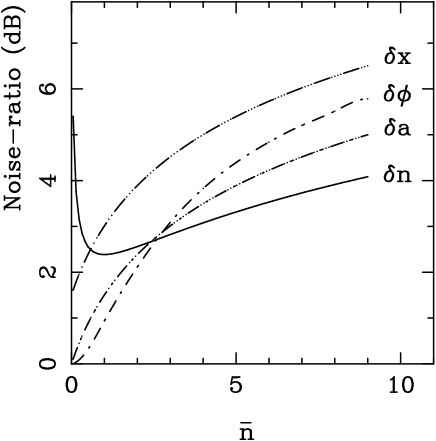
Figure 2: The noises ratio (in dB) for all the quantities considered in this paper. They are plotted for unit quantum efficiency versus $\bar{n}$: this plot has to compared with Fig. 6 of Ref. [6].

References

- [1] D. T. Smithey, M. Beck, M. G. Raymer, A. Faridani, Phys. Rev. Lett. 70, 1244 (1993).
- [2] G. M. D’Ariano, C. Macchiavello, M. G. A. Paris, Phys. Rev. A50 4298 (1994).
- [3] G. M. D’Ariano, U. Leonhardt, H. Paul, Phys. Rev. A52, R1801,(1995).
- [4] G. M. D’Ariano, in in Concepts and Advances in Quantum Optics and Spectroscopy of Solids, ed. by T. Hakioglu and A. S. Shumovsky. (Kluwer, Amsterdam 1996
- [5] D. T. Smithey, M. Beck, J. Cooper, and M. G. Raymer, Phys. Rev. A 48, 3159 (1993).
- [6] G. M. D’Ariano, C. Macchiavello, M. G. A. Paris, Phys. Lett. A195, 31 (1994).
- [7] G. M. D’Ariano, C. Macchiavello, N. Sterpi, J. Mod. Opt., to appear
- [8] G. M. D’Ariano, TOKYO
- [9] I. S. Gradshteyn, I. M. Ryzhik, Table of integral, series, and product, (Academic Press, 1980).
- [10] Th. Richter, Phys. Lett. A 221 327 (1996).
- [11] A. Orlowsky, A. Wünsche, Phys. Rev. A48 4617 (1993).
- [12] J. H. Shapiro, S. S. Wagner, IEEE J. Quantum Electron. QE20, 803 (1984); H. P. Yuen, J. H. Shapiro, IEEE Trans. Inform. Theory IT26, 78 (1980).
- [13] N.G. Walker, J.E. Carrol, Opt. Quantum Electr. 18, 355(1986); N. G. Walker, J. Mod. Opt. 34, 15 (1987).
- [14] Y. Lay, H. A. Haus, Quantum Opt. 1, 99 (1989).
- [15] G. M. D’Ariano, M. G. A. Paris, Phys. Rev. 49 3022 (1994).
- [16] A. Zucchetti, W. Vogel, D.-G. Welsch, Phys. Rev. A54 856 (1996)
- [17] M. G. A. Paris, A. Chizhov, O. Steuernagel, Opt. Comm. 134, 117 (1997).
- [18] A. S. Holevo, Probabilistic and Statistical Aspects of Quantum Theory (North-Holland Publishing, Amsterdam, 1982).
- [19] C. W. Helstrom, Quantum Detection and Estimation Theory (Academic Press, New York, 1976).
- [20] Popov V P and Yarunin V S 1992 J. Mod. Opt. 39 1525