Equivalence between Bell’s inequality and a constraint
on stochastic field theories for EPR states

Abstract

A generalized form of EPR state is defined, embracing both classical and nonclassical states. It is shown that for such states, Bell’s inequality is equivalent to a constraint on stochastic field theories. Thus, violation of Bell’s inequality can be observed also for weak violation of stochastic field theories. The Schrödinger cat state is shown to be an example of this.

I Introduction

In their classical paper [1], Einstein, Podolsky and Rosen (EPR) considered a twoparticle state. They pointed out that for a suitable choice of experimental parameters, it was possible to “predict with certainty” the outcome of a measurement on particle 2 on basis of a measurement on particle 1. They claimed that “there exists an element of physical reality corresponding to this physical quantity”. Since these elements of reality are not reflected in the theory, they concluded that quantum theory is incomplete. They saw that alternatively the reality of the second system might “depend upon the process of measurement carried out on the first system, which does not disturb the second system in any way”. This is the possibility of nonlocality, which they immediately rejected: “No reasonable definition of reality could be expected to permit this.”

EPR considered position and momentum observables, which have a continuous spectrum. Bohm reformulated the EPR problem in terms of dichotomic observables by using the singlet spin-$\frac{1}{2}$ state [2]. Also for this state it is possible to “predict with certainty” the outcome of a spin measurement on particle 2 on basis of a measurement on particle 1. A particular orientation of the spin-filters must be used to achieve this.

Bell derived a contradiction with quantum theory by using EPR’s two fundamental assumptions of locality and realism [3]. He employed the singlet spin-$\frac{1}{2}$ state introduced by Bohm.

Greenberger, Horne and Zeilinger found a contradiction between quantum theory and local realism without the use of inequalities [4]. They employed a three-particle entangled state where it was possible to “predict with certainty” the outcome of a measurement at two different locations on basis of a single measurement in a third location.

Hardy derived contradictions between quantum theory and local realism without the use of inequalities for two-particle states [5, 6]. Also here, “elements of reality” played an essential role in the derivation.

Gisin and Peres recently showed that any nonfactorable pure state violates Bell’s inequality [7]. A similar result was derived by Mann, Revzen and Schleich [8]. These proofs employ operators for which no general measurement method is known. The experimental testing of local realism has only been performed with entangled two-particle states (reviews of experiments are given in Refs. [9, 10, 11, 12]). There does not exist any general experiment which can be used to test whether an arbitrary state violates local realism.

In this paper, I consider in particular a family of states which will be called EPR states. These states allow a property of one subsystem to be predicted with certainty from a measurement on another subsystem with spacelike separation. According to the definition given here, an EPR state may be either classical or nonclassical, it may be a multiparticle state or possess an indefinite particle number, and it may be either pure or mixed. Several examples of EPR states are given, such as entangled states, single photon states, coherent states and “Schrödinger cat” states. In fact, any single mode state, pure or mixed, can be transformed into an EPR state by use of beamsplitters.

I demonstrate that any EPR state which violates an inequality for stochastic field theories also violates Bell’s inequality, and vice versa.

In stochastic field theories the Glauber-Sudarshan $P$-distribution is nonnegative and not more singular than a delta function [13]. Some quantum states violate such inequalities (reviews can be found in Refs. [14, 15]). Other researchers have found that strong violation of a Cauchy-Schwarz inequality and stochastic field theories is required to observe violation of Bell’s inequality [15, 16]. I show that violation of local realism can also be observed for weak violation of stochastic field theories.

II Elements of reality and correlation strength

In this section, I propose a definition for a generalized form of EPR states. A normalized correlation is introduced, and it is shown that the correlation strength is maximized in an EPR state. The correlation strength is expressed in terms of operators for the input channels to the interferometer.

A A general experiment

Consider the experiment depicted in Fig. 1. The lefthand and righthand side of the experiment is designated by indices $k=1$ and 2, respectively. A phase delay $\theta_{k}$ is inserted into channel $b_{k}$. Afterwards this channel is mixed with channel $a_{k}$ on a semireflecting beamsplitter $BS_{k}$, yielding output channels $c_{k}$ and $d_{k}$.

Let the photon number operator for channel $\mu_{k}$ be designated by $\hat{n}_{\mu_{k}}$ ($\mu=a,b,c,d$ and $k=1,2$). We shall say that a state is an EPR state if it is possible to find a parameter choice ($\theta_{1},\theta_{2}$) so that

$$\langle\hat{n}_{c_{1}}\hat{n}_{d_{2}}\rangle=\langle\hat{n}_{d_{1}}\hat{n}_{c_{2}}\rangle = 0,$$ (2)

$$\langle\hat{n}_{c_{1}}\hat{n}_{c_{2}}\rangle+\langle\hat{n}_{d_{1}}\hat{n}_{d_{2}}\rangle \neq 0.$$ (3)

If $\langle\hat{n}_{\mu_{1}}\hat{n}_{\nu_{2}}\rangle=0$ ($\mu,\nu=c,d$), the joint probability of finding at least one photon both in channels $\mu_{1}$ and $\nu_{2}$ vanishes. On the other hand, if $\langle\hat{n}_{\mu_{1}}\hat{n}_{\nu_{2}}\rangle>0$, this same probability is nonvanishing. Still, in the latter case, there may of course be a nonvanishing probability of finding zero photons in at least one of the two channels. On basis of these considerations, we conclude that that a state satisfying the conditions (II A) support EPR elements of reality in the following sense: If at least one photon is found in channel $c_{1}$ ($d_{1}$), it can be predicted with certainty that

• no photons will be found in channel $d_{2}$ ($c_{2}$)

• zero or more photons will be found in channel $c_{2}$ ($d_{2}$).

The maximally entangled state which is usually employed in Bell-type experiments is an EPR state according to the definition above. However, this definition even encompasses states where for a certain subsensemble no coincidences occur between the two sides of the interferometer. Moreover, we shall see that not all EPR states violate local realism. In fact, EPR states can be generated from any single-mode state. Several example states illustrating these effects will be considered in section IV.

We introduce operators for the photon number difference and the photon number sum for the output channels from beamsplitter $BS_{k}$,

$$\hat{D}_{k} = \hat{n}_{c_{k}}-\hat{n}_{d_{k}},$$ (5)

$$\hat{S}_{k} = \hat{n}_{c_{k}}+\hat{n}_{d_{k}}.$$ (6)

The correlation between the leftside and rightside interferometers can be quantified by the normalized ratio

$$E={\langle\hat{D}_{1}\hat{D}_{2}\rangle\over\langle\hat{S}_{1}\hat{S}_{2}\rangle}.$$ (7)

Since the photon number difference cannot exceed the photon number sum, the modulus of $E$ is restricted to unity,

$$\mid E\mid\leq 1.$$ (8)

Using the definitions (II A), we may write

$$E={\langle\hat{n}_{c_{1}}\hat{n}_{c_{2}}\rangle-\langle\hat{n}_{c_{1}}\hat{n}_{d_{2}}\rangle-\langle\hat{n}_{d_{1}}\hat{n}_{c_{2}}\rangle+\langle\hat{n}_{d_{1}}\hat{n}_{d_{2}}\rangle\over\langle\hat{n}_{c_{1}}\hat{n}_{c_{2}}\rangle+\langle\hat{n}_{c_{1}}\hat{n}_{d_{2}}\rangle+\langle\hat{n}_{d_{1}}\hat{n}_{c_{2}}\rangle+\langle\hat{n}_{d_{1}}\hat{n}_{d_{2}}\rangle}.$$ (9)

If the conditions (II A) are fulfilled, it follows that $E=1$.

Assume that the annihilation and creation operators for channel $\mu_{k}$ are designated by $\hat{\mu}_{k}$ and $\hat{\mu}_{k}^{{\dagger}}$, respectively. The annihilation operators for the input and output channels are connected by a unitary transformation

$$\left(\begin{array}[]{c}\hat{c}_{k}\\ \hat{d}_{k}\end{array}\right)={1\over\sqrt{2}}\left(\begin{array}[]{cc}1&1\\ -1&1\end{array}\right)\left(\begin{array}[]{cc}1&0\\ 0&e^{i\theta_{k}}\end{array}\right)\left(\begin{array}[]{c}\hat{a}_{k}\\ \hat{b}_{k}\end{array}\right).$$ (10)

Using this, the operators for the photon number difference and sum may be written as

$$\hat{D}_{k} = \hat{a}_{k}^{{\dagger}}\hat{b}_{k}e^{i\theta_{k}}+\hat{a}_{k}\hat{b}_{k}^{{\dagger}}e^{-i\theta_{k}},$$ (12)

$$\hat{S}_{k} = \hat{n}_{a_{k}}+\hat{n}_{b_{k}}.$$ (13)

Note, in particular, that only the photon number difference is modified by phase changes. It can be shown [17] that $E$ may be written in the form

$$E=A_{1}\cos(\theta_{1}-\theta_{2}+\xi)+A_{2}\cos(\theta_{1}+\theta_{2}+\zeta),$$ (14)

The coefficients $A_{k}$ will be called “correlation-amplitudes”. They are nonnegative, and defined as

$$A_{1} = {2\mid\langle\hat{a}_{1}^{{\dagger}}\hat{b}_{1}\hat{a}_{2}\hat{b}_{2}^{{\dagger}}\rangle\mid\over\langle(\hat{n}_{a_{1}}+\hat{n}_{b_{1}})(\hat{n}_{a_{2}}+\hat{n}_{b_{2}})\rangle},$$ (16)

$$A_{2} = {2\mid\langle\hat{a}_{1}^{{\dagger}}\hat{b}_{1}\hat{a}_{2}^{{\dagger}}\hat{b}_{2}\rangle\mid\over\langle(\hat{n}_{a_{1}}+\hat{n}_{b_{1}})(\hat{n}_{a_{2}}+\hat{n}_{b_{2}})\rangle},$$ (17)

where

$$\xi=\arg\langle\hat{a}_{1}^{{\dagger}}\hat{b}_{1}\hat{a}\hat{b}_{2}^{{\dagger}}\rangle,$$ (19)

$$\zeta=\arg\langle\hat{a}_{1}^{{\dagger}}\hat{b}_{1}\hat{a}_{2}^{{\dagger}}\hat{b}_{2}\rangle.$$ (20)

According to Eq. (14), $E$ can be modulated between $\pm A$, where

$$A=A_{1}+A_{2}.$$ (21)

This quantity can be regarded as a normalized measure of the correlation strength. Also, it can be seen as the total correlation amplitude. It is always nonnegative, and cannot exceed unity since the modulus of $E$ cannot exceed unity. For EPR states (II A) we have

$$A=1.$$ (22)

Conversely, if $A=1$, it can be shown that the state supports EPR elements or reality in the sense of Eq. (II A). Moreover, if $A=1$, a parameter choice can be found for which $E=-1$, and for which

$$\langle\hat{n}_{c_{1}}\hat{n}_{c_{2}}\rangle=\langle\hat{n}_{d_{1}}\hat{n}_{d_{2}}\rangle = 0,$$ (24)

$$\langle\hat{n}_{c_{1}}\hat{n}_{d_{2}}\rangle+\langle\hat{n}_{d_{1}}\hat{n}_{c_{2}}\rangle \neq 0.$$ (25)

B Homodyne detection

In the special case where the channels $b_{k}$ are coherent state local oscillators (see Fig. 2), the density operator may be written as

$$\hat{\rho}=\hat{\rho}_{a}\otimes\hat{\rho}_{b},$$ (26)

where

$$\hat{\rho}_{b}=\hat{\rho}_{b_{1}}\otimes\hat{\rho}_{b_{2}}$$ (27)

and

$$\hat{\rho}_{b_{k}}=\mid\beta_{k}e^{i\theta_{k}}\rangle_{b_{k}}\quad{}_{b_{k}}{\langle\beta_{k}e^{i\theta_{k}}\mid}.$$ (28)

Now the local oscillator phases $\theta_{k}$ play the role of local parameters. The amplitudes $\beta_{k}$ may be chosen to be real, and it can be shown [17, 18] that $E$ is maximized by the choice

$$\beta_{1}\beta_{2} = \sqrt{\langle\hat{n}_{a_{1}}\hat{n}_{a_{2}}\rangle},$$ (30)

$${\beta_{1}\over\beta_{2}} = \sqrt{{\langle\hat{n}_{a_{1}}\rangle\over\langle\hat{n}_{a_{2}}\rangle}}.$$ (31)

This leads to the following form [18] for the correlation amplitudes $A_{k}$,

$$A_{1}={\mid g^{(1,1)}\mid\over 1+\sqrt{g^{(2,2)}}},$$ (33)

$$A_{2}={\mid g^{(2,0)}\mid\over 1+\sqrt{g^{(2,2)}}},$$ (34)

where

$$g^{(1,1)} = {\langle\hat{a}_{1}^{{\dagger}}\hat{a}_{2}\rangle\over\sqrt{\langle\hat{n}_{a_{1}}\rangle\langle\hat{n}_{a_{2}}\rangle}},$$ (36)

$$g^{(2,0)} = {\langle\hat{a}_{1}^{{\dagger}}\hat{a}_{2}^{{\dagger}}\rangle\over\sqrt{\langle\hat{n}_{a_{1}}\rangle\langle\hat{n}_{a_{2}}\rangle}},$$ (37)

$$g^{(2,2)} = {\langle\hat{a}_{1}^{{\dagger}}\hat{a}_{2}^{{\dagger}}\hat{a}_{2}\hat{a}_{1}\rangle\over\langle\hat{n}_{a_{1}}\rangle\langle\hat{n}_{a_{2}}\rangle}.$$ (38)

We see that the correlation amplitudes $A_{k}$ can be defined in terms of Glauber coherence functions [19]. In particular, $g^{(1,1)}$ and $g^{(2,2)}$ are known as the degree of first and second order coherence (also sometimes called the degree of second and fourth order coherence). They can be observed, e.g., as the interference visibility and the coincidence rate in a Mach-Zehnder interferometer.

III Correlation inequalities

In this section, inequalities are derived for the correlation amplitudes $A_{k}$ in stochastic field theories, locally realistic theories and quantum theory. The connection between the inequalities is discussed, particularly for EPR states.

A An inequality for stochastic field theories

In appendix A, it is shown that stochastic field theories impose the restrictions

$$A_{k}\leq{1\over 2}\quad(k=1,2).$$ (39)

Thus stochastic field theories restrict each correlation amplitude in itself. Both amplitudes may reach the maximal value of $1/2$ simultaneously. This is seen, e.g., in a coherent state.

B Bell’s inequality

It has been shown that in local, realistic theories, the quantity

$$B=E(\theta_{1},\theta_{2})-E(\theta_{1}^{\prime},\theta_{2})+E(\theta_{1},\theta_{2}^{\prime})+E(\theta_{1}^{\prime},\theta_{2}^{\prime})$$ (40)

is restricted by the condition [9, 15]

$$\mid B\mid\leq 2.$$ (41)

Tan et al. [17] showed that by a proper choice of phases $\theta_{k}$, the maximal value of $B$ is

$$B_{\max}=2\sqrt{2}\>\sqrt{A_{1}^{2}+A_{2}^{2}}.$$ (42)

It follows that local realism is violated unless

$$A_{1}^{2}+A_{2}^{2}\leq{1\over 2}.$$ (43)

This is a necessary but not sufficient condition for a state to be describable in terms of a local, hidden variable theory.

C Quantum inequalities

If no interconnection existed between the four terms in the expression $B$ in Eq. (40), it would have a maximum of 4. However, we saw that in locally realistic theories the maximum is 2, and it follows from the considerations above that the same limit applies in stochastic field theories. Tsirelson showed that in quantum theory the allowed maximum is [20]

$$\mid B\mid\leq 2\sqrt{2}.$$ (44)

It follows from (42) that Tsirelson’s inequality can be written as

$$A_{1}^{2}+A_{2}^{2}\leq 1.$$ (45)

This is a necessary, but not a sufficient condition on the amplitudes $A_{k}$. A necessary and sufficient condition within quantum theory is found by combining Eqs. (8) and (21),

$$A_{1}+A_{2}\leq 1.$$ (46)

D Comparison of the inequalities

The inequalities (39), (43), (45) and (46) have been illustrated in Fig. 3. We see that stochastic field theories allow the smallest range of amplitudes $A_{k}$. Within locally realistic theories, a larger range of amplitudes is allowed, and an even larger range of amplitudes is permitted in quantum theory. The widest range of amplitudes is allowed by the Tsirelson inequality, but it is seen to permit amplitudes forbidden by quantum theory.

It is interesting to note that the limits imposed by stochastic field theories, local realism and quantum theory intersect in the point $A_{1}=A_{2}=1/2$. Note furthermore that EPR states are represented by the limit line for quantum theory. Thus we see that any EPR state for which $A_{k}\neq 1/2$ violates both local realism and stochastic field theories.The farther away from the central point $A_{1}=A_{2}=1/2$, the stronger the violation.

If we consider states where one amplitude $A_{k}$ is zero, the maximal amplitude allowed by stochastic field theories is $1/2$, in locally realistic theories it is $1/\sqrt{2}$ and in quantum theory it is 1. This is somewhat reminiscent of the result found by Su and Wódkiewicz [16]. They examined the interference visibility of the intensity correlation in two-photon experiments, and found that stochastic field theories restricts this visibility to $1/2$, local realism to $1/\sqrt{2}$ and quantum theory to 1. Their conclusion was that violation of local realism requires strong violation of classical field theory. This is in agreement with the results found here, provided that one amplitude $A_{k}$ vanishes. For an entangled two-photon state, one of the amplitudes $A_{k}$ must vanish (see Sec. IV). However, Fig. 3 shows that in EPR states, violation of local realism can be observed also for weak violation of stochastic field theories.

Another interesting observation is that if one of the amplitudes $A_{k}$ exceeds the limit of $1/2$ imposed by stochastic field theories, then according to the quantum limit (46) the other amplitude must be smaller than $1/2$. Thus, although quantum theory allows the amplitudes to exceed the classical limit (39), it instead imposes a complementarity relation (46) between the two.

IV Some EPR states

In this section, various EPR states are considered. They are mostly well known, some classical and some nonclassical.

The section is divided into two subsections for two different experimental setups; a general setup (Fig. 1) and a setup using coherent local oscillators (Fig. 2). The task is essentially to describe possible contents in the “black boxes” in Figs. 1 and 2.

A The general setup

1 An arbitrary single mode state

Consider an arbitrary single mode state, pure or mixed. Assume that this state is first mixed with vacuum on a semireflecting beamsplitter (see Fig. 4). Next, assume that each output channel from this beamsplitter is again mixed with vacuum on a semireflecting beamsplitter. It can then be shown (see App. B) that this produces an EPR state with the properties $A_{1}=A_{2}=\frac{1}{2}$. Such states therefore are classical in the sense that they do not violate the Cauchy-Schwarz and Bell inequalities (39) and (43).

It is interesting that a highly coherent state can be produced from any single mode state. This shows that a quantized field behaves in many ways just like a classical field.

2 Entangled states

A maximally entangled state can be written as [21]

$$\mid\psi\rangle={1\over\sqrt{2}}( \mid 1\rangle_{a_{1}}\otimes\mid 0\rangle_{b_{1}}\otimes\mid 1\rangle_{a_{2}}\otimes\mid 0\rangle_{b_{2}}$$ (47)

$$+ \mid 0\rangle_{a_{1}}\otimes\mid 1\rangle_{b_{1}}\otimes\mid 0\rangle_{a_{2}}\otimes\mid 1\rangle_{b_{2}}).$$ (48)

The photons are either in channel $a_{1}$ and $a_{2}$ or in channels $b_{1}$ and $b_{2}$. This is equivalent to the situation in the singlet spin-$\frac{1}{2}$ state, where either the left spin is up and the right is down or vice versa. For this state, $A_{1}=0$ and $A_{2}=1$. Thus the state is both an EPR state and it yields maximal violation of local realism. An equivalent maximally entangled state is

$$\mid\psi\rangle={1\over\sqrt{2}}( \mid 1\rangle_{a_{1}}\otimes\mid 0\rangle_{b_{1}}\otimes\mid 0\rangle_{a_{2}}\otimes\mid 1\rangle_{b_{2}}$$ (49)

$$+ \mid 0\rangle_{a_{1}}\otimes\mid 1\rangle_{b_{1}}\otimes\mid 1\rangle_{a_{2}}\otimes\mid 0\rangle_{b_{2}}).$$ (50)

Here the photons are either in channel $a_{1}$ and $b_{2}$ or $b_{1}$ and $a_{2}$. For this state, $A_{1}=1$ and $A_{2}=0$.

3 Two independent photons

Consider the two-photon state

$$\mid\psi\rangle=\mid 1\rangle\>\otimes\mid 1\rangle.$$ (51)

Such states can be generated, e.g., in parametric down-conversion. Due to the product form, the two photons are independent. Assume that each photon is mixed with vacuum on a beamsplitter (cf. Fig. 5). In terms of output states from the beamsplitter, this may be written

$$\mid\psi\rangle=\frac{1}{2}(\mid 1\rangle_{a_{1}}\otimes\mid 0\rangle_{a_{2}}+\mid 0\rangle_{a_{1}}\otimes\mid 1\rangle_{a_{2}} )$$ (52)

$$\otimes(\mid 1\rangle_{b_{1}}\otimes\mid 0\rangle_{b_{2}}+\mid 0\rangle_{b_{1}}\otimes\mid 1\rangle_{b_{2}} )$$ . (53)

This is still a product state between the $a$- and $b$-channels. There has been some discussion whether such states can violate local realism, the argument being that it is really generated from a product state [22, 23]. However, the $a$-channels are later pairwise mixed with $b$-channels, and there is no longer a product form between eigenstates for the left and right sides of the interferometer. Here it is found that $A_{1}=1$, $A_{2}=0$. Thus this is an EPR state which violates local realism maximally. Note that EPR elements of reality can only be predicted in 50% of the outcomes, because in the rest 50% of the outcomes, the two photons will go to the same side of the interferometer.

B A setup with local oscillators

1 Coherent states

For coherent states

$$\mid\psi\rangle_{a}=\mid\alpha_{1}\rangle_{a_{1}}\otimes\mid\alpha_{2}\rangle_{a_{2}}$$ (54)

we find that $\mid g^{(1,1)}\mid=\mid g^{(2,0)}\mid=g^{(2,2)}=1$. It therefore follows from Eqs. (II B) that $A_{k}=1/2$. Thus, coherent states are EPR states, and they neither violate Bell’s inequality (43) nor the constraint (39) on stochastic field theories. This is in agreement with the conclusions in Ref. [8].

2 A split single photon

Consider the split single photon state [17, 24, 25, 26]

$$\mid\psi\rangle_{a}={1\over\sqrt{2}}\left(\mid 1\rangle_{a_{1}}\otimes\mid 0\rangle_{a_{2}}+\mid 0\rangle_{a_{1}}\rangle_{b_{1}}\otimes\mid 1\rangle_{a_{2}}\right).$$ (55)

It yields $g^{(1,1)}=1$, $g^{(2,0)}=0$, $g^{(2,2)}=0$, and thus $A_{1}=1$, $A_{2}=0$. Thus it yields a strong violation both of local realism and of stochastic field thories.

Note that according to the conditions (II B), the local oscillator amplitudes should vanish. This is not possible in practice if the purpose is to measure $E$, since then no coincidences occur at all. However, for sufficiently small local oscillator amplitudes, the state behaves “almost” as an EPR state [25].

3 A split “Schrödinger cat”

As an example of an EPR state yielding both weak violation of Bell’s inequality and the constraint (39) on stochastic field theories, consider the state

$$\mid\psi\rangle_{a}=N\,\left(\mid\alpha\rangle_{a_{1}}\>\otimes\mid\alpha\rangle_{a_{2}}+e^{i\phi}\mid-\alpha\rangle_{a_{1}}\>\otimes\mid-\alpha\rangle_{a_{2}}\right),$$ (56)

where the normalization constant is

$$N=\left[\,2\left(1+e^{-4\mid\alpha\mid^{2}\,}\cos\phi\right)\right]^{-1/2}.$$ (57)

These states can be generated from a “Schrödinger cat state” [27]

$$\mid\psi\rangle=N\,\left(\,\mid\sqrt{2}\alpha\rangle+e^{i\phi}\mid-\sqrt{2}\alpha\rangle\,\right)$$ (58)

by mixing with vacuum at a semireflecting beamsplitter. For parameter choices $\phi=0$ and $\phi=\pi$ we have even and odd coherent states [28], while $\phi=\pi/2$ yield “Yurke-Stoler” states [27]. Atomic Schrödinger cat states have recently been generated experimentally [29, 30]. It can be shown that

$$g^{(1,1)} = 1,$$ (60)

$$g^{(2,0)} = {1+e^{-4\mid\alpha\mid^{2}}\cos\phi\over 1-e^{-4\mid\alpha\mid^{2}}\cos\phi},$$ (61)

$$g^{(2,2)} = \left(g^{(2,0)}\right)^{2}.$$ (62)

By inserting into Eqs. (II B), it follows that

$$A_{1} = {1\over 2}\left(1-e^{-4\mid\alpha\mid^{2}}\cos\phi\right),$$ (64)

$$A_{2} = {1\over 2}\left(1+e^{-4\mid\alpha\mid^{2}}\cos\phi\right).$$ (65)

It is easily seen that

$$A_{1}+A_{2}=1.$$ (66)

The Schrödinger cat states are therefore EPR states, regardless of the phase choice $\phi$. It also follows that

$$A_{1}^{2}+A_{2}^{2}={1\over 2}\left[1+e^{-8\mid\alpha\mid^{2}}\cos^{2}\phi\right].$$ (67)

Thus, both Bell’s inequality and inequality (39) are violated for any choice of parameters except when $\phi=\pi/2$. Even if the parameters are chosen so that only a weak violation of stochastic field theories and inequality (39) takes place, Bell’s inequality is also violated. Note, however, that although these states display a small violation of local realism even for macroscopic amplitudes $\mid\alpha\mid$, this violation vanishes exponentially. Therefore, these states are not suitable for demonstrating violation of local realism in macroscopic states.

V Conclusion

It has been shown that violation of local realism can be observed also for weak violation of classical field theories. It was shown that Bell’s inequality is equivalent to a constraint on classical field theories.

Violation of local realism requires that a certain two-point correlation is stronger than classically [31]. However, it also requires that another correlation form is reduced below the classical limit, as was shown in this paper.

The Bell inequality used in this paper involves an additional assumption related to the “no-enhancement assumption” [9, 15, 32, 33]. Therefore, the experiments discussed in this paper may rule out only hidden variable theories which fulfill this assumption. This is a common feature of all Bell inequalities that have been experimentally tested so far. Inequalities derived without this assumption in general require higher detector efficiencies in order to be tested [9, 34].

There exist EPR states which display nonclassical properties but which nevertheless do not violate the constraint (39) on classical theories. An example of this is the split Yurke-Stoler state (see section IV B 3). Such states of course do not violate the Bell-inequality (43) either. Thus, the experiment presented here does not demonstrate violation of local realism of every nonclassical EPR state. However, if the EPR state violates the classical inequality (39), it also violates the Bell inequality (43).

It should be noted that whereas a classical Glauber-Sudarshan $P$- distribution is a sufficient condition for a state to obey local realism, a nonclassical $P$-distribution is in general only a necessary and not a sufficient condition for the violation of local realism. One may imagine, e.g., a product state where either of the sub-states possess some highly nonclassical $P$-distribution. Such a state does not violate any Bell inequality [7].

A Constraint on stochastic field theories

The density operator for the experiment shown in Fig. 1 may be represented in terms of a Glauber-Sudarshan quasi-distribution $P(\alpha_{1},\alpha_{2},\beta_{1},\beta_{2})$ as

$$\hat{\rho} = \int P(\alpha_{1},\alpha_{2},\beta_{1},\beta_{2})\mid\alpha_{1}\rangle_{a_{1}}\>{}_{a_{1}}{\langle\alpha_{1}\mid}\>\otimes\mid\alpha_{2}\rangle_{a_{2}}\>{}_{a_{2}}{\langle\alpha_{2}\mid}$$ (A1)

$$\otimes \mid\beta_{1}\rangle_{b_{1}}\>{}_{b_{1}}{\langle\beta_{1}\mid}\>\otimes\mid\beta_{2}\rangle_{b_{2}}\>{}_{b_{2}}{\langle\beta_{2}\mid}\>d^{2}\alpha_{1}\>d^{2}\alpha_{2}\>d^{2}\beta_{1}\>d^{2}\beta_{2}.$$ (A2)

According to Eqs. (II A), the amplitudes $A_{k}$ may be written as

$$A_{1} = {2\mid\int P(\alpha_{1},\alpha_{2},\beta_{1},\beta_{2})\alpha_{1}^{*}\beta_{1}\alpha_{2}^{*}\beta_{2}\>d^{2}\alpha_{1}\>d^{2}\alpha_{2}\>d^{2}\beta_{1}\>d^{2}\beta_{2}\mid\over\int P(\alpha_{1},\alpha_{2},\beta_{1},\beta_{2})(\mid\alpha_{1}\mid^{2}+\mid\beta_{1}\mid^{2})(\mid\alpha_{2}\mid^{2}+\mid\beta_{2}\mid^{2})\>d^{2}\alpha_{1}\>d^{2}\alpha_{2}\>d^{2}\beta_{1}\>d^{2}\beta_{2}},$$ (A4)

$$A_{2} = {2\mid\int P(\alpha_{1},\alpha_{2},\beta_{1},\beta_{2})\alpha_{1}^{*}\beta_{1}^{*}\alpha_{2}\beta_{2}\>d^{2}\alpha_{1}\>d^{2}\alpha_{2}\>d^{2}\beta_{1}\>d^{2}\beta_{2}\mid\over\int P(\alpha_{1},\alpha_{2},\beta_{1},\beta_{2})(\mid\alpha_{1}\mid^{2}+\mid\beta_{1}\mid^{2})(\mid\alpha_{2}\mid^{2}+\mid\beta_{2}\mid^{2})\>d^{2}\alpha_{1}\>d^{2}\alpha_{2}\>d^{2}\beta_{1}\>d^{2}\beta_{2}}.$$ (A5)

For any complex numbers $\alpha_{k}$ and $\beta_{k}$ the inequality

$$\mid\alpha_{k}\mid^{2}+\mid\beta_{k}\mid^{2}\>\geq\>2\mid\alpha_{k}\beta_{k}\mid$$ (A6)

applies. This inequality was recently used to demonstrate a nonclassical two-photon effect [35, 36]. If the state can be described in terms of stochastic field theories, the $P$-distribution is nonnegative and not more singular than a delta-function [13]. For such $P$-distributions it follows that

$$A_{1}\> \leq \>{\mid\int P(\alpha_{1},\alpha_{2},\beta_{1},\beta_{2})\alpha_{1}^{*}\beta_{1}\alpha_{2}^{*}\beta_{2}\>d^{2}\alpha_{1}\>d^{2}\alpha_{2}\>d^{2}\beta_{1}\>d^{2}\beta_{2}\mid\over 2\int P(\alpha_{1},\alpha_{2},\beta_{1},\beta_{2})4\mid\alpha_{1}\alpha_{2}\beta_{1}\beta_{2}\mid\>d^{2}\alpha_{1}\>d^{2}\alpha_{2}\>d^{2}\beta_{1}\>d^{2}\beta_{2}},$$ (A8)

$$A_{2}\> \leq \>{\mid\int P(\alpha_{1},\alpha_{2},\beta_{1},\beta_{2})\alpha_{1}^{*}\beta_{1}^{*}\alpha_{2}\beta_{2}\>d^{2}\alpha_{1}\>d^{2}\alpha_{2}\>d^{2}\beta_{1}\>d^{2}\beta_{2}\mid\over 2\int P(\alpha_{1},\alpha_{2},\beta_{1},\beta_{2})4\mid\alpha_{1}\alpha_{2}\beta_{1}\beta_{2}\mid\>d^{2}\alpha_{1}\>d^{2}\alpha_{2}\>d^{2}\beta_{1}\>d^{2}\beta_{2}},$$ (A9)

and finally

$$A_{k}\leq{1\over 2},\quad(k=1,2).$$ (A10)

B Splitting of an arbitrary single-mode state

Consider an arbitrary single mode state, defined in terms of the Sudarshan $P$-distribution as

$$\hat{\rho}_{1}=\int P(\alpha)\mid\alpha\rangle\langle\alpha\mid d^{2}\alpha.$$ (B1)

Assume that this state is mixed with vacuum on a semireflecting beamsplitter, the total density operator being $\hat{\rho}_{2}=\hat{\rho}_{1}\otimes\mid 0\rangle\langle 0\mid$ (cf. Fig. 4). A coherent state is transformed according to

$$\mid\alpha\rangle\>\otimes\mid 0\rangle=\mid{\alpha\over\sqrt{2}}\rangle\>\otimes\mid{\alpha\over\sqrt{2}}\rangle,$$ (B2)

where the right side is expressed in terms of output states. Thus the density operator $\hat{\rho}_{2}$ can be expressed in terms of the output states as

$$\hat{\rho}_{2}=\int P(\alpha)\mid{\alpha\over\sqrt{2}}\rangle\langle{\alpha\over\sqrt{2}}\mid\otimes\mid{\alpha\over\sqrt{2}}\rangle\langle{\alpha\over\sqrt{2}}\mid d^{2}\alpha.$$ (B3)

Next, each output channel is again mixed with vacuum on a semireflecting beamsplitter (cf. Fig. 4), the total density operator now becoming

$$\hat{\rho}_{4}=\rho_{2}\>\otimes\mid 0\rangle\langle 0\mid\otimes\mid 0\rangle\langle 0\mid.$$ (B4)

In terms of the output states, the density operator then may be written as

$$\hat{\rho}_{4}=\int P(\alpha)\mid{\alpha\over 2}\rangle_{a_{1}}\>{}_{a_{1}}\langle{\alpha\over 2}\mid\otimes\mid{\alpha\over 2}\rangle_{b_{1}}\>{}_{b_{1}}\langle{\alpha\over 2}\mid\otimes\mid{\alpha\over 2}\rangle_{a_{2}}\>{}_{a_{2}}\langle{\alpha\over 2}\mid\otimes\mid{\alpha\over 2}\rangle_{b_{2}}\>{}_{b_{2}}\langle{\alpha\over 2}\mid d^{2}\alpha,$$ (B5)

or, by a change of integration variables,

$$\hat{\rho}_{4}=4\int P(2\beta)\mid\beta\rangle_{a_{1}}\>{}_{a_{1}}\langle\beta\mid\otimes\mid\beta\rangle_{b_{1}}\>{}_{b_{1}}{\langle}\beta\mid\otimes\mid\beta\rangle_{a_{2}}\>{}_{a_{2}}\langle\beta\mid\otimes\mid\beta\rangle_{b_{2}}\>{}_{b_{2}}\langle\beta\mid d^{2}\beta.$$ (B6)

We now may find the numerator and denominator for the amplitudes $A_{k}$ in Eqs. (II A). We thus find that

$$\langle (\hat{a}_{1}^{{\dagger}}\hat{a}_{1}+\hat{b}_{1}^{{\dagger}}\hat{b}_{1})(\hat{a}_{2}^{{\dagger}}\hat{a}_{2}+\hat{b}_{2}^{{\dagger}}\hat{b}_{2})\rangle=\mathrm{Tr}\>\left[\rho_{4}\>(\hat{a}_{1}^{{\dagger}}\hat{a}_{1}+\hat{b}_{1}^{{\dagger}}\hat{b}_{1})(\hat{a}_{2}^{{\dagger}}\hat{a}_{2}+\hat{b}_{2}^{{\dagger}}\hat{b}_{2})\right]$$ (B7)

$$= 16\>\mathrm{Tr}\>[\int P(2\beta)\mid\beta\mid^{4}\>\mid\beta\rangle_{a_{1}}\>{}_{a_{1}}\langle\beta\mid\otimes\mid\beta\rangle_{b_{1}}\>{}_{b_{1}}{\langle}\beta\mid\otimes\mid\beta\rangle_{a_{2}}\>{}_{a_{2}}\langle\beta\mid\otimes\mid\beta\rangle_{b_{2}}\>{}_{b_{2}}\langle\beta\mid d^{2}\beta\>].$$ (B8)

Likewise, we find that

$$2 \mid\langle\hat{a}_{1}^{{\dagger}}\hat{b}_{1}\hat{a}_{2}^{{\dagger}}\hat{b}_{2}\rangle\mid=2\mid\mathrm{Tr}\>\left[\rho_{4}\>\hat{a}_{1}^{{\dagger}}\hat{b}_{1}\hat{a}_{2}^{{\dagger}}\hat{b}_{2}\right]\mid$$ (B9)

$$= 8\>\mathrm{Tr}\>[\int P(2\beta)\mid\beta\mid^{4}\>\mid\beta\rangle_{a_{1}}\>{}_{a_{1}}\langle\beta\mid\otimes\mid\beta\rangle_{b_{1}}\>{}_{b_{1}}{\langle}\beta\mid\otimes\mid\beta\rangle_{a_{2}}\>{}_{a_{2}}\langle\beta\mid\otimes\mid\beta\rangle_{b_{2}}\>{}_{b_{2}}\langle\beta\mid d^{2}\beta\>]$$ (B10)

and

$$2 \mid\langle\hat{a}_{1}^{{\dagger}}\hat{b}_{1}^{{\dagger}}\hat{a}_{2}\hat{b}_{2}\rangle\mid=2\mid\mathrm{Tr}\>\left[\rho_{4}\>\hat{a}_{1}^{{\dagger}}\hat{b}_{1}^{{\dagger}}\hat{a}_{2}\hat{b}_{2}\right]\mid$$ (B11)

$$= 8\>\mathrm{Tr}\>[\int P(2\beta)\mid\beta\mid^{4}\>\mid\beta\rangle_{a_{1}}\>{}_{a_{1}}\langle\beta\mid\otimes\mid\beta\rangle_{b_{1}}\>{}_{b_{1}}{\langle}\beta\mid\otimes\mid\beta\rangle_{a_{2}}\>{}_{a_{2}}\langle\beta\mid\otimes\mid\beta\rangle_{b_{2}}\>{}_{b_{2}}\langle\beta\mid d^{2}\beta\>].$$ (B12)

It thus follows that

$$\langle(\hat{a}_{1}^{{\dagger}}\hat{a}_{1}+\hat{b}_{1}^{{\dagger}}\hat{b}_{1})(\hat{a}_{2}^{{\dagger}}\hat{a}_{2}+\hat{b}_{2}^{{\dagger}}\hat{b}_{2})\rangle=4\mid\langle\hat{a}_{1}^{{\dagger}}\hat{b}_{1}\hat{a}_{2}^{{\dagger}}\hat{b}_{2}\rangle\mid=4\mid\langle\hat{a}_{1}^{{\dagger}}\hat{b}_{1}^{{\dagger}}\hat{a}_{2}\hat{b}_{2}\rangle\mid,$$ (B13)

and, by substituting into Eqs. (II A), we conclude that

$$A_{k}=\frac{1}{2}\quad(k=1,2).$$ (B14)

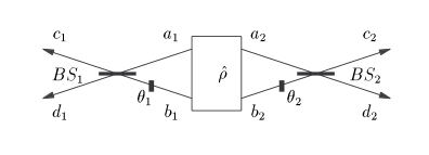
FIG. 1.: A general Bell experiment.

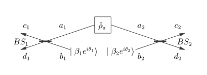
FIG. 2.: A Bell experiment involving two local oscillators.

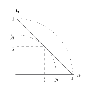
FIG. 3.: The limits on the correlation amplitudes $A_{k}$. Solid line: Constraint on quantum theory. This line also defines EPR states. Dashed line: Constraint on stochastic field theories. Dash-dotted line: Bell’s inequality. Dotted line: Tsirelson’s inequality.

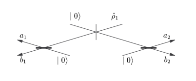
FIG. 4.: Splitting of an arbitrary single mode state to produce an EPR state

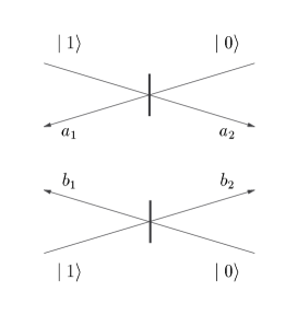
FIG. 5.: Generating an EPR state from two independent photons

REFERENCES

• [1] A. Einstein, B. Podolsky, and N. Rosen, Phys. Rev. 47, 777 (1935).
• [2] D. Bohm, Quantum Theory (Prentice-Hall, New York, 1951).
• [3] J. S. Bell, Physics (Long Island City, N.Y.) 1, 195 (1964).
• [4] D. M. Greenberger, M. A. Horne, and A. Zeilinger, in Bell’s Theorem, Quantum Theory and Conceptions of the Universe, edited by M. Kafatos (Kluwer Academic Publishers, Dordrecht, 1989), pp. 69–72.
• [5] L. Hardy, Phys. Rev. Lett. 68, 2981 (1992).
• [6] L. Hardy, Phys. Lett. 167, 17 (1992).
• [7] N. Gisin and A. Peres, Phys. Lett. A 162, 15 (1992).
• [8] A. Mann, M. Revzen, and W. Schleich, Phys. Rev. A 46, 5363 (1992).
• [9] J. F. Clauser and A. Shimony, Rep. Prog. Phys. 41, 1881 (1978).
• [10] L. E. Ballentine, Am. J. Phys. 55, 785 (1987).
• [11] D. Home and F. Selleri, Nuovo Cimento 14, 1 (1991).
• [12] R. Y. Chiao, P. G. Kwiat, and A. M. Steinberg, Quant. Semiclass. Opt. 7, 259 (1995).
• [13] L. Mandel and E. Wolf, in Optical Coherence and Quantum Optics (Cambridge University Press, New York, 1995), Chap. 11.8, pp. 540–541.
• [14] R. Loudon, Rep. Prog. Phys. 43, 913 (1980).
• [15] M. D. Reid and D. F. Walls, Phys. Rev. A 34, 1260 (1986).
• [16] C. Su and K. Wódkiewicz, Phys. Rev. A 44, 6097 (1991).
• [17] S. M. Tan, M. J. Holland, and D. F. Walls, Opt. Commun. 77, 285 (1990).
• [18] L. M. Johansen, Phys. Lett. A 219, 15 (1996).
• [19] R. J. Glauber, Phys. Rev. 130, 2529 (1963).
• [20] B. S. Cirel’son, Lett. Math. Phys. 4, 93 (1980).
• [21] M. A. Horne, A. Shimony, and A. Zeilinger, Phys. Rev. Lett. 62, 2209 (1989).
• [22] L. De Caro and A. Garuccio, Phys. Rev. A 50, R2803 (1994).
• [23] P. G. Kwiat, Phys. Rev. A 52, 3380 (1995).
• [24] B. J. Oliver and C. R. Stroud Jr., Phys. Lett. A 135, 407 (1989).
• [25] S. M. Tan, D. F. Walls, and M. J. Collett, Phys. Rev. Lett. 66, 252 (1991).
• [26] L. Hardy, Phys. Rev. Lett. 73, 2279 (1994).
• [27] B. Yurke and D. Stoler, Phys. Rev. Lett. 57, 13 (1986).
• [28] V. V. Dodonov, I. A. Malkin, and V. I. Man’ko, Physica 72, 597 (1974).
• [29] C. Monroe, D. M. Meekhof, B. E. King, and D. J. Wineland, Science 272, 1131 (1996).
• [30] M. W. Noel and C. R. Stroud, Jr., Phys. Rev. Lett. 77, 1913 (1996).
• [31] A. Peres, Am. J. Phys. 46, 745 (1978).
• [32] E. Santos, Phys. Rev. Lett. 68, 894 (1992).
• [33] S. M. Tan, D. F. Walls, and M. J. Collett, Phys. Rev. Lett. 68, 895 (1992).
• [34] A. Garg and N. D. Mermin, Phys. Rev. D 35, 3831 (1987).
• [35] J. D. Franson, Phys. Rev. Lett. 67, 290 (1991).
• [36] J. D. Franson, Phys. Rev. A 44, 4552 (1991).
Refer to caption