Quantum computation with phase drift errors.

Abstract

We present results of numerical simulations of the evolution of an ion trap quantum computer made out of $18$ ions which are subject to a sequence of nearly $15000$ laser pulses in order to find the prime factors of $N=15$. We analyze the effect of random and systematic phase drift errors arising from inaccuracies in the laser pulses which induce over (under) rotation of the quantum state. Simple analytic estimates of the tolerance for the quality of driving pulses are presented. We examine the use of watchdog stabilization to partially correct phase drift errors concluding that, in the regime investigated, it is rather inefficient.

2

The key ingredient for quantum computation is the use of quantum parallelism which takes advantage of the fact that the dimensionality of the Hilbert space of the computer is exponentially dependent on its physical size. Feynman [1] pointed out that classical computers are intrinsically inefficient when simulating the dynamics of a quantum system since for a chain of $L$ spins we need to store $O(2^{L})$ complex amplitudes in memory. Since this quantity scales exponentially with the size, he reasoned, a quantum computer would be much more efficient requiring, as nature does, only $O(L)$ sites. Shor’s discovery [2] of a quantum algorithm for efficient factoring of integers is solid evidence that quantum computers could exponentially outperform their classical counterparts in problems which are not motivated by quantum mechanics per se. The last two years have witnessed an intense research effort aimed at examining the possibilities for taking quantum computation from the realm of ideas to the real world of the laboratory. However, practical implications of a “quantum revolution” for computation are still not clear. In this work we will analyze the performance of the ion–trap quantum information processor [3], which is currently under study by various experimental groups around the world (see [4] for a review). For concreteness we analyze the evolution of a quantum computer which runs a program to find the prime factors of a small number ($N=15$). Such program can be best represented by a quantum circuit decomposing into a complex sequence of elementary gates, i.e. unitary operations affecting qubits individually or in pairs [5]. In our simulations, which tested several factoring circuits [6], we followed the quantum state of $n_{i}=18$ cold trapped ions subject to a predetermined sequence of $n_{p}\approx 15000$ (resonant and off–resonant) laser pulses.

These simulations face the same problem which prompted Feynman to propose the use of quantum computers in the first place: As their Hilbert space increases exponentially with their size, any dynamical study rapidly becomes a very hard computational task. Thus, to our knowledge, evolution corresponding to factoring in the proposed implementations of quantum computers has never been simulated beyond the level of a few qubits or small fragments of the complete algorithm [3]. Here, we present the first results of large numerical simulation of an ion trap quantum computer evolving under realistic (but still rather oversimplified) conditions.

We aim at examining the tolerance of quantum computation to errors which are likely to occur in any optically driven quantum–processor. In fact, for quantum gates to properly operate, most laser pulses are designed to invert population between internal levels ($\pi$–pulses). However, the Rabi flopping frequency depends on a variety of physical effects which cause imperfections: Realistic $\pi$–pulses (or any other type of pulse) will always be $(\pi+\epsilon)$–pulses, being $\epsilon$ a random variable whose expectation value $\bar{\epsilon}$ and dispersion $\sigma$ characterize the quality of the experimental setup. In our study we analyzed the impact of these timing errors showing that a successful quantum computation (even on a rather small scale) imposes stringent limitations in the quality of laser pulses. Perhaps most importantly, we obtained and verified simple analytic expressions that could be used for estimating the fidelity of the final state of the computer. Our results make evident that error correction and fault tolerant computation [7] are necessary for successfully implementing simple circuits. These techniques would make posible arbitrarily large computations if the precision of the driving laser pulses are above a certain threshold. Unfortunately, simulating circuits which incorporate quantum error correcting codes is still beyond our capabilities: encoding a single qubit into $k$ (which should be at least 3) makes the time and memory requirements to grow by a factor $2^{k}$.

We have also set out to test the effectiveness of the watchdog (or quantum Zeno) effect for error correction. The basic physics of this effect is rather well known: Consider a two level system which is initially in state $|0\rangle$ and is subject to a sequence of rotations by an angle $\theta$. After $k$ such rotations the probability for measuring the initial state is $P(0)=\cos^{2}(k\theta)$, which vanishes when $k\theta=\pi/2$. However, measuring the state after each rotation tends to slow down evolution: the probability for finding the qubit always in state $|0\rangle$ is $P_{w}(0)=\cos^{2k}(\theta)$, which is close to one if $\theta$ is sufficiently small. At first sight, using this quantum Zeno effect to stabilize a quantum computation may seem implausible since to implement it one would have to know the ideal state of the computer at some times. However in an ideal factoring circuit, some of the qubits disentangle from the rest of the computer at predetermined steps of the algorithm allowing for watchdog stabilization. With our simulations we tested this simple idea confirming the existence of watchdog stabilization but concluding that the technique is rather inefficient in the ion trap quantum computer.

In this implementation each qubit is stored in the internal levels of a single ion. Ions are linearly trapped and laser cooled to their translational ground state (in the Lamb–Dicke limit). Two long-lived atomic ground states $|g\rangle$ and $|e\rangle$ of each ion play the role of the computational states (an additional auxiliary level $|e^{\prime}\rangle$ is needed for implementing quantum gates). Each ion can be addressed by a laser and Rabi oscillations between the two computational states can be induced by tunning the laser frequency to the energy difference $\hbar\omega$ between ground and excited state. In this case, the quantum state of the qubit evolves as $|\Psi(t)\rangle=U(t)|\Psi(0)\rangle$, where the matrix of $U(t)$ in the $(|g\rangle,|e\rangle)$ basis is:

$$U(t)=\left(\begin{array}[]{cc}\cos\Omega t&-ie^{-i\Phi}\sin\Omega t\\ -ie^{i\Phi}\sin\Omega t&\cos\Omega t\\ \end{array}\right)$$ (1)

Thus, controlling the Rabi frequency $\Omega$, the laser phase $\Phi$ and the pulse duration $t$, arbitrary single qubit rotations can be performed. To implement two-bit gates one induces interactions between qubits using the center of mass mode as an intermediary: Applying a laser pulse to ion $n$ with a frequency $\omega-\nu$, where $\hbar\nu$ is the energy of a single phonon of the CM mode, Rabi oscillations are induced between states $|g\rangle_{\text{n}}|1\rangle_{\text{CM}}$ and $|e\rangle_{\text{n}}|0\rangle_{\text{CM}}$. For these states the evolution operator is also (1), while states $|g\rangle_{\text{n}}|0\rangle_{\text{CM}}$ and $|e\rangle_{\text{n}}|1\rangle_{\text{CM}}$ remain unchanged by the interaction. These off-resonance pulses allow swapping information to and from the center of mass conditioned on the state of the $n$th qubit. As Cirac and Zoller showed [3], by combining the two types of pulses applied on two different ions (and using an auxiliary level as a kind of “work–space”) universal quantum gates can be implemented. Errors in $\Omega t$ and $\Phi$, such as the ones arising from fluctuations in the laser intensity which produce variations of $\Omega$, will result in over(under) rotations. Such phase drift errors are the ones of concern here. Other sources of errors, such us the decoherence of the CM mode or the spontaneous decay of the ions, will be ignored. In effect we assume that the computer evolves isolated from the environment being affected only by unitary errors.

The factoring circuit is based on Shor’s algorithm [2]. Prime factors of $N$ are found by obtaining the order $r$ of a number $y$ which is coprime with $N$. This is the smallest integer such that $y^{r}=1\ \text{mod}\ N$ (with $r$ one computes the greatest common divisor between $N$ and $x^{r/2}-1$, which is a factor of $N$ whenever $r$ is even and $x^{r/2}\neq 1\ \text{mod}\ N$). To find $r$ one first chooses $y$ at random and starts the computer in state $|\Psi_{0}\rangle={1\over\sqrt{q}}\sum_{j=0}^{q-1}|j\rangle_{1}|0\rangle_{2}$. Here, $|j\rangle_{1,2}$ represent two registers of the computer whose states are defined by the binary representation of $j$ ($q$ must be between $N^{2}$ and $2N^{2}$). Then, by applying a unitary transformation mapping state $|j\rangle_{1}|0\rangle_{2}$ onto $|j\rangle_{1}|y^{j}\,\text{mod}\,N\rangle_{2}$, the state of the computer is transformed into $|\Psi_{1}\rangle={1\over\sqrt{q}}\sum_{j=0}^{q-1}|j\rangle_{1}|y^{j}\,\text{mod}\,N\rangle_{2}$. Finally, one Fourier transforms the first register and measures it. The probability $P(c)$ for the outcomes of such measurement, whose analytic expression can be derived using standard quantum mechanics, is a strongly peaked distribution with the peaks separated by a multiple of $1/r$. Thus, measuring the distance between peaks one efficiently gets information about $r$ (see Fig. 1.b).

The most complicated part of the various factoring circuits [6] is the modular exponentiation section (Fourier transform can be efficiently implemented as shown in [8]). The complexity of the modular exponentiation network is such that the circuit involves $O(100)L^{3}$ elementary two bit gates [6] (the two registers of the computer require $2L$ and $L$ qubits respectively). As unitary operators are invertible, the circuit must use reversible logic for which one needs a number of extra “work–qubits” in intermediate steps of the calculation. For the simplest circuits, such number is $2L+1$. However, other networks reduce the size of the workspace enlarging the number of operations. For example, another circuit we investigated has $L+1$ work–qubits but requires $O(10)L^{5}$ elementary operations (notably, for small numbers this circuit outperforms all others both in space and time). We will not discuss any circuit details here. For the purpose of analising the physical constraints implied by efficient factoring on the accuracy of laser pulses it is sufficient to say that the simulations were performed on circuits involving the following characteristics: 18 two level ions were subjected to 15000 laser pulses ($\sim 10^{4}$ off–resonant and $\sim 5\times 10^{3}$ resonant). Eight of these ions were used in the first register, four in the second and six were used as work–qubits. If all degrees of freedom are taken into account the Hilbert space of the computer is $2\times 3^{18}$ dimensional (each ion contributes with three levels and the CM is effectively two dimensional). Unfortunately, this is too much for a classical computer. However, if we consider all pulses involving the auxiliary level $|e^{\prime}\rangle$ of each ion as perfect a substantial saving is achieved. In this case, the effective dimension of the Hilbert space is $2^{19}$ which allows for numerical simulations. Taking this into account, the erroneous pulses amount to 75% - 80% of the total. The errors in $\Omega t$ and $\Phi$ were taken as random variables normally distributed with dispersion $\sigma$ and mean $\bar{\epsilon}$.

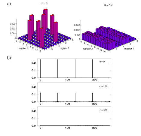
FIG. 1.: a) Probability for a measurement of the two registers of a factoring computer. After an error–free modular exponentiation circuit, the computer should be in a superposition of the form $|j\rangle|y^{j}\,\text{mod}\,N\rangle$. As $y=7$, the only states present should be: $|0\rangle|1\rangle$, $|1\rangle|7\rangle$, $|2\rangle|4\rangle$, etc (left figure). Timing errors distributed with dispersion $\sigma=5\%$ produce a probability showing no resemblance to the ideal one. b) Probability of measuring a value in the first register after Fourier transform for $\sigma=0,\ 1$ and $5\%$. For the last case all periodicity is lost and a uniform distribution arises. If $\sigma\mathchoice{\mathrel{\vbox{\hbox{$\buildrel\displaystyle<\over{\displaystyle\sim}$}}}}{\mathrel{\vbox{\hbox{$\buildrel\textstyle<\over{\textstyle\sim}$}}}}{\mathrel{\vbox{\hbox{$\buildrel\scriptstyle<\over{\scriptstyle\sim}$}}}}{\mathrel{\vbox{\hbox{$\buildrel\scriptscriptstyle<\over{\scriptscriptstyle\sim}$}}}}1\%$ the distribution shows minor changes in amplitude.

An illustrative example of the data we computed can be seen in Fig. 1 where we represent the joint probability for measuring the two registers of the computer in values $(a,x)$ before the Fourier transform is calculated (Fig. 1.b shows the distribution after Fourier transform is applied). For the case of no systematic error ($\bar{\epsilon}=0$) it is clear that a dispersion of $5\%$ in the accuracy of the pulses completely wipes out the signal one wants to observe (note that the signal disappears before applying the FT circuit. As discussed in [3] the FT circuit is quite resistant to this level of errors but our result shows that, unfortunately, this is not the case for modular exponentiation where many more operations are needed). A reasonable parameter quantifying the accuracy of the quantum computer is the fidelity, which is defined as the overlap between the actual state (obtained after evolution subject to noise) and the ideal one: $F=|\langle\Psi_{\text{actual}}|\Psi_{\text{ideal}}\rangle|^{2}$. Our observations show that a fidelity below $1/5$ implies the loss of the signal one wants to observe (in general $F$ is closely related to the probability of observing the system in the correct state, i.e. measuring the first register on a peak in Fig. 1b). In Fig. 2 we show the dependence of fidelity upon the dispersion of the errors. The numerical results follow remarkably well a simple formula that can be derived by assuming one has $l$ independent qubits each one of which is subject to $n/l$ erroneous pulses. In this way (treating the center of mass motion separately, as it is subject to a larger number of pulses) we conclude that the mean fidelity (averaging over the ensemble of errors) is

$$\bar{F}=\left[{1\over 2}\left(1+e^{-2n_{\text{t}}\sigma^{2}/l}\right)\right]^{l}\ \left[{1\over 2}\left(1+e^{-2\sigma^{2}n_{\text{cm}}}\right)\right],$$ (2)

where $n_{\text{t}}$ is the total number of pulses and $n_{\text{cm}}$ is the number of off-resonance ones (which involve the center of mass). This rough estimate was also used to estimate the dependence of the fidelity on the number of operations (for fixed dispersion $\sigma$) giving also good quantitative agreement with the simulations. We numerically computed a fidelity for every realization of the noise finding the average over many (i.e. a few tens) noise realizations. Error bars in Figure 2 correspond to the dispersion around the mean of the numerically computed result. Fortunately, fluctuations are relatively small and therefore each run gives a reasonable idea of the average result. The reason for this is that each run corresponds to a random choice of many (nearly $15000$) independent random variables. Therefore, fluctuations between different runs are effectively suppressed.

It is also interesting to estimate the number of dimensions explored by the state of the computer, which while moving on a large Hilbert space is subject to random perturbations. For this purpose we computed the entropy of the density matrix $\rho_{\text{av}}$, obtained by averaging the state vector on the ensemble of noise realizations. Linear entropy $S_{\text{lin}}=-\log_{2}(\,\text{Tr}\,\rho_{\text{av}}^{2}\,)$ (which provides a simple lower bound to von–Neumann entropy) turns out to be well approximated by:

$$S_{\text{lin}}=l+1-\log_{2}\left[(1+e^{-4n_{\text{t}}\sigma^{2}/l})^{l}(1+e^{-4n_{\text{cm}}\sigma^{2}})\right].$$ (3)

This equation was shown to agree with numerical results and predicts that for dispersions above a few percents the computer explores the entire available Hilbert space (enough statistics to numerically test the above formula was only gathered for dispersions below $2\%$).

FIG. 2.: Fidelity as a function of the noise dispersion $\sigma$ (for $\bar{\epsilon}=0$) at the end of the modular exponentiation circuit for factoring $N=15$ (with $q=256$ and $y=7$). The dashed line is the naïve qualitative estimate given by equation (2) with $n_{\text{t}}=1.5\times 10^{4}$, $n_{\text{cm}}=10^{4}$.

To analyze the effectiveness of watchdog stabilization we simulated a smaller version of our factoring $N=15$ circuit with only the first three controlled multipliers. In these simulations we assumed a systematic error using $\bar{\epsilon}=1.1\sigma$. Whenever a work–qubit was expected to be in a state $|0\rangle$ a measurement was performed on it. As the center of mass is supposed to return to the ground state after each gate, a measurement of its state was also carried out (in practice this could be done using a “red light ion” as suggested in [10]). The probability for finding all these qubits in the correct state was recorded and the computation was continued on the correct branches only. The final fidelity, defined as the probability for the sequence of correct results, was computed and compared with the previously described one (when no watchdog was performed). The simulations show that watchdog stabilization produces a minor improvement in the fidelity: For example, when $\sigma=0.1\%$ the fidelity with watchdog was 0.67 as opposed to 0.64 without it. To estimate the improvement one should expect we computed the fidelity of $l$ independent qubits which are subject to watchdog stabilization after each of $n/l$ rotations by an angle $\bar{\epsilon}$. In this case, the result is rather surprising: this ideal watchdog would produce a fidelity close to $0.99$, a number which is much larger than the one computed numerically. This inefficiency of the stabilization method can be explained as follows: Measuring the state of a few qubits (the ones that disentangle from the rest of the computer at some intermediate times) one is doing a “partial watchdog”. Thus, after the measurement we know with certainty that the measured qubits are in the “correct” state but the rest of the computer may be in an erroneous one. To test this simple explanation we run a numerical simulation where, after each measurement, the state of the computer was projected onto the ideal one. In this case, the agreement with the naïve (independent qubit) estimate was good being the fidelity close to $0.99$.

One of the interesting results of our study is that, although the factoring circuit continuously correlates the qubits, the dependence of fidelity on the noise parameters, can be estimated using a simple model where non–systematic errors affect each qubit independently (with this model, equation (2) can be easily obtained). However, for purely systematic errors ($\sigma=0$) we were not able to obtain a simple analytic estimate for the fidelity fitting the results of our simulations. For example, assuming that every qubit evolves independently under the influence of $n/l$ pulses which produce a rotation in an angle $\bar{\epsilon}$ one gets a formula for the mean fidelity which differs from eq. (2) by a term $\cos 2\bar{\epsilon}n/l$ multiplying each exponential. This naïve estimate predicts a lower fidelity than the one we numerically computed. The reason for this seems to be the existence of cancellations of errors associated, in a nontrivial way, with the reversible nature of the circuit (for example, in a controlled not gate systematic errors exactly cancel when the control qubit is in the ground state but propagate otherwise). This suggests that pulse sequences implementing logic gates should be designed to properly compensate for systematic over(under) rotations. If this is achieved, the remaining fidelity is well approximated by equation (2).

We acknowledge the hospitality of the ITP at Santa Barbara where this work was completed. This research was supported in part by the NSF grant No. PHY94–07194. JPP was also supported by grants from UBACyT, Fundación Antorchas and Conicet (Argentina).

REFERENCES

- [1] R. Feynman, Int. J. Theo. Phys., 21, 467 (1982).
- [2] P. W. Shor, in Proceedings of the 35th Annual Symposium on Foundations of Computer Science. edited by S.Goldwasser (IEEE Computer Society, Los Alamitos, CA, 1994), p. 116.
- [3] J. I. Cirac and P. Zoller, Phys. Rev. Lett.74, 4091 (1995).
- [4] A. Steane, Report No. quant-ph/9608011.
- [5] A. Barenco, et. al., Phys. Rev. A52, 3457 (1994).
- [6] C. Miquel, J.P. Paz and R. Perazzo, Phys. Rev. A54, 2605 (1996); V. Vedral, A. Barenco and A. Ekert, Phys. Rev. A54, 139 (1996); D. Beckman, A. N. Chari, S. Devabhaktumi, J. Preskill, Phys. Rev. A54, 1034; E. Knill, Private communication.
- [7] P. Shor, Phys. Rev. A(1995); A. Steane, Phys. Rev. Lett.77, 793 (1996); R. Laflamme, C. Miquel, J. P. Paz and W. Zurek, Phys. Rev. Lett.77, 198 (1996); C. Bennet D.P. DiVincenzo, J.A. Smolin and W.K. Wooters, Phys. Rev. A54, 3824 (1996); E. Knill and R. Laflamme (1996) Report No. quant-ph/9604034.
- [8] R. B. Griffiths and C. Niu, Phys. Rev. Lett.76, 3228 (1996)
- [9] W. H. Zurek, Phys. Rev. Lett.53, 391 (1984)
- [10] J. I. Cirac, T. Pellizzari and P. Zoller, Science, 273, 1207 (1996).
- [11] W. H. Zurek, Phys. Today 44, 36 (1991).