FSUJ TPI QO-2/97

March, 1997

Photon-added state preparation via conditional measurement on a beam splitter
M. Dakna, L. Knöll, D.–G. Welsch
Friedrich-Schiller-Universität Jena Theoretisch-Physikalisches Institut

Max-Wien Platz 1, D-07743 Jena, Germany

Abstract

We show that conditional output measurement on a beam splitter may be used to produce photon-added states for a large class of signal-mode quantum states, such as thermal states, coherent states, squeezed states, displaced photon-number states, and coherent phase states. Combining a mode prepared in such a state and a mode prepared in a photon-number state, the state of the mode in one of the output channels of the beam splitter “collapses” to a photon-added state, provided that no photons are detected in the other output channel. We present analytical and numerical results, with special emphasis on photon-added coherent and squeezed vacuum states. In particular, we show that adding photons to a squeezed vacuum yields superpositions of quantum states which show all the typical features of Schrödinger-cat-like states.

1 Introduction

It is well known that according to von Neumann’s projection principle [1] conditional measurement may be a fruitful method for quantum-state manipulation and engineering. In particular, when a system, such as a correlated two-mode optical field or a correlated atom-field system, is prepared in an entangled state of two subsystems and a measurement is performed on one subsystem, then the quantum state of the other subsystem can be reduced to a new state. Systems that have typically been considered are the waves produced by parametric amplifiers [2, 3, 4] and degenerate four-wave mixers [5], the interfering fields in the output channels of a beam splitter [4, 6], and systems of the Jaynes-Cummings type in cavity QED [7] or trapped-ion studies [8]. Further, state reduction via continuous measurement has also been considered [9, 10, 11, 4]. Conditional measurement offers new possibilities of generating extremely nonclassical states, such as photon-number states [5, 8, 10, 12, 13] and Schrödinger-cat-like states [3, 11, 14].

In this paper we show that zero-photon conditional output measurement on a beam splitter can be used advantageously to generate photon-added states for a large class of quantum states of the signal mode, such as thermal states, coherent states, squeezed states, displaced photon-number states, coherent phase states etc.. It can be expected that repeated application of the photon creation operator to the signal-mode quantum state can produce extremely nonclassical states. Photon adding can therefore be expected to improve the performance of noise reduction schemes [15]. In particular, the states that are obtained from coherent states by repeatedly applying to them the photon creation operator – the photon-added coherent states – can be regarded as non-Gaussian squeezed states and were first introduced and discussed in [16] and it was proposed that they can be produced in nonlinear processes in cavities. We show that photon-added coherent states can also be generated via conditional output measurement on a beam splitter, mixing a signal mode prepared in a coherent state with a second mode prepared in a photon-number state.

We further show that when a signal mode prepared in a squeezed vacuum is mixed with photon-number states and zero-photon conditional output measurements are performed, then photon-added squeezed vacuum states can be produced. We analyze the states in terms of the photon-number and quadrature-component distributions and the Wigner and Husimi functions. We show that photon-added squeezed vacuum states exhibit all the typical properties of Schrödinger-cat-like states, so that photon adding can be regarded as a method for producing Schrödinger cats. In particular, they are shown to be superpositions of two non-Gaussian squeezed coherent states that tend to Gaussian squeezed coherent states for sufficiently large number of added photons. It is worth noting that although the scheme bears some resemblance to that in [14], the two schemes are quite different from each other. That concerns both the second input quantum state (which is the vacuum in [14]) and the conditional output measurement (detection of a nonzero number of photons in [14]).

The paper is organized as follows. In Sec. 2 the basic scheme is explained and the conditional output states are derived. The possibility of the generation of photon-added states is studied in Sec. 3, with special emphasis on photon-added coherent and squeezed vacuum states. The problem of mixed photon-added states is addressed in Sec. 4. A summary and concluding remarks are given in Sec. 5.

2 Basis equations

It is well known that the input–output relations at a lossless beam splitter can be characterized by the $\rm SU(2)$ Lie algebra [17, 18]. In the Heisenberg picture, the photon destruction operators of the outgoing modes, $\hat{b}_{k}$ ($k\!=\!1,2$), can be obtained from those of the incoming modes, $\hat{a}_{k}$, as

$$\hat{b}_{k}=\sum_{k^{\prime}=1}^{2}T_{k,k^{\prime}}\,\hat{a}_{k^{\prime}},$$ (1)

where

$$(T_{k,k^{\prime}})=e^{i\varphi_{0}}\left(\begin{array}[]{cc}\cos\theta\;e^{i\varphi_{T}}&\sin\theta\;e^{i\varphi_{R}}\\ -\sin\theta\;e^{-i\varphi_{R}}&\cos\theta\;e^{-i\varphi_{T}}\end{array}\right)$$ (4)

is a SU(2) matrix whose elements are given by the complex transmittance $T$ and reflectance $R$ of the beam splitter,

$$T=\cos\theta\;e^{i\varphi_{T}},\quad R=\sin\theta\;e^{i\varphi_{R}}.$$ (5)

Using the Schrödinger picture, the photonic operators are left unchanged, but the density operator is transformed. In this case the output-state density operator $\hat{\varrho}_{\rm out}$ can be related to the input-state density operator $\hat{\varrho}_{\rm in}$ as

$$\hat{\varrho}_{\rm out}=\hat{V}^{\dagger}\hat{\varrho}_{\rm in}\hat{V},$$ (6)

where $\hat{V}$ can be given by [17, 18]

$$\hat{V}=e^{-i(\varphi_{T}-\varphi_{R})\hat{L}_{3}}\,e^{-2i\theta\hat{L}_{2}}\,e^{-i(\varphi_{T}+\varphi_{R})\hat{L}_{3}},$$ (7)

with

$$\hat{L}_{2}=\textstyle\frac{1}{2i}(\hat{a}_{1}^{\dagger}\hat{a}_{2}-\hat{a}_{2}^{\dagger}\hat{a}_{1}),\quad\hat{L}_{3}=\textstyle\frac{1}{2}(\hat{a}_{1}^{\dagger}\hat{a}_{1}-\hat{a}_{2}^{\dagger}\hat{a}_{2}).$$ (8)

Note that $\varphi_{0}$ is a global phase factor that may be omitted without loss of generality, $\varphi_{0}\!=\!0$. Applying elementary parameter-differentiation techniques [19], we can derive the operator identity

$$e^{-2i\theta\hat{L}_{2}}=e^{\tan(\theta)\hat{a}_{2}^{\dagger}\hat{a}_{1}}\,e^{2\ln\cos(\theta)\hat{L}_{3}}\,e^{-\tan(\theta)\hat{a}_{1}^{\dagger}\hat{a}_{2}},$$ (9)

which [together with Eq. (5)] enables us to rewrite $\hat{V}^{\dagger}$, Eq. (7), as

$$\hat{V}^{\dagger}=T^{\hat{n}_{1}}\,e^{-R^{*}\hat{a}^{\dagger}_{2}\hat{a}_{1}}\,e^{R\hat{a}^{\dagger}_{1}\hat{a}_{2}}\,T^{-\hat{n}_{2}}\,,$$ (10)

where $\hat{n}_{k}=\hat{a}^{\dagger}_{k}\hat{a}_{k}$.

Now, let us assume (Fig. 1) that the modes that are fed into the first and second input channels of the beam splitter are prepared in a state described by a density operator $\hat{\varrho}_{{\rm in}1}$ and a Fock state $\hat{\varrho}_{{\rm in}2}$ $\!=$ $\!|n_{0}\rangle\langle n_{0}|$, respectively (for a review on the problem of the generation of Fock states, see [20]). The input-state density operator can then be written as

$$\hat{\varrho}_{\rm in}(n_{0})=\hat{\varrho}_{{\rm in}1}\otimes|n_{0}\rangle\langle\,n_{0}|.$$ (11)

Using Eqs. (6), (10), and (11), after some calculation the output-state density operator $\hat{\varrho}_{\rm out}$ $\!\equiv$ $\!\hat{\varrho}_{\rm out}(n_{0})$ can be given by

$$\hat{\varrho}_{\rm out}(n_{0})=\frac{1}{|T|^{2n_{0}}}\sum_{n_{2}=0}^{\infty}\sum_{m_{2}=0}^{\infty}\sum_{k=0}^{n_{0}}\sum_{j=0}^{n_{0}}(R^{*})^{m_{2}+j}R^{n_{2}+k}$$ (12)

$$\times\frac{(-1)^{n_{2}+m_{2}}}{\sqrt{k!j!m_{2}!n_{2}!}}\sqrt{\!{n_{0}\choose k}\!{n_{0}\choose j}\!{n_{0}\!-\!k\!+\!m_{2}\choose m_{2}}\!{n_{0}\!-\!j\!+\!n_{2}\choose n_{2}}}$$

$$\times\,T^{\hat{n}_{1}}{\hat{a}_{1}}^{m_{2}}({\hat{a}_{1}^{\dagger}})^{k}\hat{\varrho}_{{\rm in}1}\hat{a}_{1}^{j}({\hat{a}_{1}^{\dagger}})^{n_{2}}(T^{*})^{\hat{n}_{1}}\otimes|n_{0}-k+m_{2}\rangle\langle n_{0}-j+n_{2}|.$$

It can easily be seen that when the second input channel is unused, i.e., $n_{0}$ $\!=$ $\!0$, then Eq. (12) reduces to the relation considered in [4, 6, 14].

From Eq. (12) we see that the output modes are, in general, highly correlated. When the photon number of the mode in the second output channel is measured and $m_{2}$ photons are detected, then the mode in the first output channel is prepared in a quantum state whose density operator $\hat{\varrho}_{{\rm out}1}(n_{0},m_{2})$ reads as

$$\hat{\varrho}_{{\rm out}1}(n_{0},m_{2})=\frac{\langle m_{2}|\hat{\varrho}_{\rm out}(n_{0})|m_{2}\rangle}{{\rm Tr}_{1}(\langle m_{2}|\hat{\varrho}_{\rm out}(n_{0})|m_{2}\rangle)}\,.$$ (13)

The probability of such an event is given by

$$P(n_{0},m_{2})={\rm Tr}_{1}(\langle m_{2}|\hat{\varrho}_{\rm out}{(n_{0})}|m_{2}\rangle)=\!\!\sum_{n_{1}=\mu-\nu}^{\infty}\sum_{j=\mu}^{n_{0}}\sum_{k=\mu}^{n_{0}}\;\!\!|R|^{2(j+k-\nu)}|T|^{2(n_{1}+\nu-n_{0})}$$ (14)

$$\times\,\frac{(-1)^{j+k}n_{0}!\,n{{}_{1}}!}{(n_{1}+\nu)!(n_{0}-\nu)!}{n_{0}-\nu\choose j-\nu}{n_{0}-\nu\choose k-\nu}{n_{1}+j\choose j}{n_{1}+k\choose k}\langle n_{1}|\hat{\varrho}_{{\rm in}1}|n_{1}\rangle,$$

where

$$\nu=n_{0}-m_{2},\;\mu=\max(0,\nu).$$ (15)

3 Generation of photon-added states

Let us now assume that the (signal) mode in the first input channel is prepared in a mixed state

$$\hat{\varrho}_{{\rm in}1}=\sum_{\Phi}\tilde{p}_{\Phi}\,|\Phi\rangle\langle\Phi|$$ (16)

($\sum_{\Phi}\tilde{p}_{\Phi}$ $\!=$ $\!1$, $0$ $\!\leq$ $\!\tilde{p}_{\Phi}$ $\!\leq$ $\!1$) and restrict attention to the events that no photons are recorded in the second output channel, i.e.,

$$m_{2}=0,\qquad\nu=n_{0}$$ (17)

in Eqs. (12) – (14). Note that such events can be detected using highly efficient avalanche photodiodes. Combining Eqs. (12) and (13) and using Eqs. (16) and (17), we find that the mode in the first output channel is prepared in a state

$$\hat{\varrho}_{{\rm out}1}(n_{0},m_{2}=0)=\sum_{\Phi}\tilde{p}_{\Phi}|\,\Psi_{n_{0}}\rangle\big{\langle}\Psi_{n_{0}}|\,,$$ (18)

where

$$|\Psi_{n_{0}}\rangle=\frac{1}{\sqrt{{\cal N}_{n_{0}}}}\,(\hat{a}^{\dagger}_{1})^{n_{0}}\,T^{\hat{n}_{1}}|\Phi\rangle,$$ (19)

${\cal N}_{n_{0}}$ being a normalization constant,

$${\cal N}_{n_{0}}=\langle\Phi|(T^{\ast})^{\hat{n}_{1}}\hat{a}_{1}^{n_{0}}(\hat{a}^{\dagger}_{1})^{n_{0}}T^{\hat{n}_{1}}|\Phi\rangle.$$ (20)

The probability of observing the conditional state $\hat{\varrho}_{{\rm out}1}(n_{0},m_{2}=0)$ can easily be found from Eq. (14) and reads

$$P(n_{0})\equiv P(n_{0},m_{2}=0)|R|^{2n_{0}}\sum_{n_{1}=0}^{\infty}|T|^{2n_{1}}{n_{1}+n_{0}\choose n_{0}}\langle n_{1}|\hat{\varrho}_{{\rm in}1}|n_{1}\rangle.$$ (21)

The states $|\Psi_{n_{0}}\rangle$, Eq. (19), are obviously the conditional states observed in the case when the mode in the first input channel is prepared in a pure state $|\Phi\rangle$. From Eq. (19) we see that for chosen $n_{0}$ the conditional state $|\Psi_{n_{0}}\rangle$ is a photon-added state, with $n_{0}$ photons being added to the state $|\Psi\rangle$ $\!\sim$ $\!T^{\hat{n}_{1}}|\Phi\rangle$. In particular when the absolute value of the transmittance is close to unity, $|T|$ $\!\approx$ $\!1$, then the state $|\Psi\rangle$ is – apart from a rotation in the phase space – close to the input state $|\Phi\rangle$. To be more specific, let us consider the expansion of $|\Phi\rangle$ in the Fock basis,

$$|\Phi\rangle=\sum_{n_{1}=0}^{\infty}c_{n_{1}}|n_{1}\rangle,$$ (22)

and assume that

$$c_{n_{1}}\approx 0\quad{\rm for}\quad n_{1}>n_{\rm max}.$$ (23)

We see that (apart from the rotation mentioned) $|\Psi\rangle$ $\!\approx$ $|\Phi\rangle$, provided that

$$|T|^{n_{1}}\approx 1\quad{\rm for}\quad n_{1}\leq n_{\rm max}.$$ (24)

Note that for any physical state $|\Phi\rangle$ the expansion in Eq. (22) can always be approximated to any desired degree of accuracy by truncating it at $n_{\rm max}$ if $n_{\rm max}$ is suitably large.

However, there are classes of states for which the corresponding photon-added states can be produced even when $|T|$ is not close to unity. Let us consider a class of $\alpha$ parametrized states $|\Phi(\alpha)\rangle$ such that

$$|\Phi(\alpha)\rangle=\sum_{n_{1}=0}^{\infty}c_{n_{1}}(\alpha)|n_{1}\rangle,\quad{\rm with}\quad c_{n_{1}}(\alpha)\propto\alpha^{n_{1}}.$$ (25)

Since in this case the relation $|\Psi\rangle$ $\!\sim$ $\!T^{\hat{n}_{1}}|\Phi(\alpha)\rangle$ $\!=$ $\!|\Phi(T\alpha)\rangle$ is valid, the state $|\Psi\rangle$ obviously belongs to the class of states $|\Phi(\alpha)\rangle$. Hence when the input state $|\Phi\rangle$ belongs to the class of states $|\Phi(\alpha)\rangle$, then the conditional output state

$$|\Psi_{n_{0}}\rangle\sim(\hat{a}^{\dagger})^{n_{0}}|\Psi\rangle\sim(\hat{a}^{\dagger})^{n_{0}}|\Phi(T\alpha)\rangle$$ (26)

is a photon-added states, with the photons being added to a state $|\Psi\rangle$ that also belongs to the class of states $|\Phi(\alpha)\rangle$. The extension of the above given considerations to mixed states is straightforward. Typical examples of classes of photon-added states that can be produced in this way are thermal states, coherent states, squeezed states, displaced Fock states, and coherent phase states.

When the number of added photons, $n_{0}$, is sufficiently small compared to the photon numbers that mainly contribute to the state $|\Psi\rangle$ and the photon-number distribution $|\langle n_{1}|\Psi\rangle|^{2}$ is sufficiently slowly varying with $n_{1}$, then the photon-added state $|\Psi_{n_{0}}\rangle$ exhibits, in general, properties that are similar to those of the state $|\Psi\rangle$. Writing

$$|\Psi_{n_{0}}\rangle\sim(\hat{a}^{\dagger})^{n_{0}}|\Psi\rangle\sim\sum_{n_{1}=0}^{\infty}\frac{\tilde{c}_{n_{1}}}{\tilde{c}_{n_{1}+n_{0}}}\,\tilde{c}_{n_{1}+n_{0}}\left[\frac{(n_{1}+n_{0})!}{n_{1}!}\right]^{1/2}|n_{1}+n_{0}\rangle$$ (27)

($\tilde{c}_{n_{1}}$ $\!=$ $\!T^{n_{1}}c_{n_{1}}$) and using the approximations

$$\frac{\tilde{c}_{n_{1}}}{\tilde{c}_{n_{1}+n_{0}}}\approx 1,\quad\left[\frac{(n_{1}+n_{0})!}{n_{1}!}\right]^{1/2}\approx(\bar{n})^{n_{0}/2},$$ (28)

we approximately derive

$$|\Psi_{n_{0}}\rangle\sim|\Psi\rangle\sim\sum_{n_{1}=0}^{\infty}\tilde{c}_{n_{1}}|n_{1}\rangle,$$ (29)

i.e., photon adding leaves the state $|\Psi\rangle$ nearly unchanged. With increasing number of added photons qualitatively new properties are expected to be observed. To illustrate the method, let us consider photon-added coherent and squeezed vacuum states in more detail.

3.1 Coherent states

Let us first assume that the input field is prepared in a coherent state, i.e., $\hat{\varrho}_{{\rm in}1}$ $\!=$ $\!|\Phi\rangle\langle\Phi|$, where

$$|\Phi\rangle\equiv|\beta\rangle=e^{-|\beta|^{2}/2}\sum_{n=0}^{\infty}\frac{\beta^{n}}{\sqrt{n!}}\,|n\rangle,$$ (30)

with $\beta=|\beta|e^{\varphi_{\beta}}$. According to Eq. (19), the conditional output states then reads

$$|\Psi_{n_{0}}\rangle=\frac{1}{\sqrt{{\cal N}^{\prime}_{n_{0}}}}(\hat{a}^{\dagger})^{n_{0}}|\beta^{\prime}\rangle,$$ (31)

where $\beta^{\prime}$ $\!=$ $\!T\beta$ and

$${\cal N}^{\prime}_{n_{0}}=n_{0}!\,{\rm L}_{n_{0}}\!\left(-|\beta^{\prime}|^{2}\right),$$ (32)

${\rm L}_{n_{0}}(x)$ being the Laguerre polynomial. The states are photon-added coherent states and can be represented in the Fock basis as

$$|\Psi_{n_{0}}\rangle=\frac{e^{-|\beta^{\prime}|^{2}/2}}{\sqrt{{\cal N}^{\prime}_{n_{0}}}}\sum_{n=0}^{\infty}\frac{(\beta^{\prime})^{n}}{\sqrt{n!}}\left[\frac{(n+n_{0})!}{n!}\right]^{1/2}|n+n_{0}\rangle.$$ (33)

From Eqs. (21) and (30), the probability of producing photon-added coherent states is given by

$$P(n_{0})=|R|^{2n_{0}}e^{-|\beta|^{2}}\sum_{n=0}^{\infty}{n+n_{0}\choose n_{0}}\frac{|\beta^{\prime}|^{2n}}{n!}\,.$$ (34)

Using the relations [21]

$${\rm L}_{n_{0}}^{n}(0)={n+n_{0}\choose n_{0}}$$ (35)

and

$$\sum_{n=0}^{\infty}{\rm L}_{n_{0}}^{n}(x)\frac{z^{n}}{n!}=e^{z}{\rm L}_{n_{0}}(x-z)$$ (36)

(${\rm L}_{n_{0}}^{n}(x)$ is the associated Laguerre polynomial), we find that

$$P(n_{0})=|R|^{2n_{0}}e^{-|R|^{2}|\beta|^{2}}{\rm L}_{n_{0}}(-|\beta^{\prime}|^{2}).$$ (37)

In Fig. 2 the probability $P(n_{0})$ is plotted for two values of the beam-splitter transmittance $|T|$. If $|T|$ and/or $n_{0}$ are not too small, $P(n_{0})$ as a function of $|\beta|$ can attain a maximum, the position of which is determined by the (positive) solution of the equation

$$\left|T\right|^{2}{\rm L}_{n_{0}}(-|\beta^{\prime}|^{2})=\left|R\right|^{2}{\rm L}_{n_{0}-1}^{1}(-|\beta^{\prime}|^{2}).$$ (38)

We see that even if $|\beta|$ or $n_{0}$ are increased the probability $P(n_{0})$ for detecting zero photons may increase due to destructive interference. In particular Fig. 2(b) reveals that the maximum is shifted towards larger values of $|\beta|$ when $n_{0}$ is increased. For example, assuming a highly transmitting beam splitter such that $|T|^{2}$ $\!=$ $\!0.99$, probabilities $P(n_{0})$ of about of $10$% may be possible, provided that $|\beta|$ and $n_{0}$ are sufficiently large ($|\beta|$ $\!\approx$ $\!40$, $n_{0}$ $\!\approx$ $\!20$).

Photon-added coherent states (31) were introduced and studied in detail in [16], with special emphasis on their nonclassical properties, such a squeezing and sub-Poissonian photon statistics (for their quantum-phase statistics, see [23]). In particular, in [16] analytical results for the Wigner and Husimi functions are given. We therefore may restrict attention to the quadrature-component distribution (i.e., the phase-parametrized field-strength distribution)

$$p_{n_{0}}(x,\varphi)=|\langle x,\varphi|\Psi_{n_{0}}\rangle|^{2},$$ (39)

which can be measured in balanced homodyne detection. For this purpose we expand the eigenvectors $|x,\varphi\rangle$ of the quadrature components

$$\hat{x}(\varphi)=2^{-1/2}\left(e^{-i\varphi}\hat{a}+e^{i\varphi}\hat{a}^{\dagger}\right)$$ (40)

in the photon-number basis [24],

$$|x,\varphi\rangle=(\pi)^{-1/4}\exp\!\left(-\textstyle\frac{1}{2}x^{2}\right)\sum_{n=0}^{\infty}\frac{e^{in\varphi}}{\sqrt{2^{n}n!}}\,{\rm H}_{n}(x)|n\rangle$$ (41)

(H_n is the Hermite polynomial). Using the identity [21]

$$\sum_{k=0}^{\infty}\frac{z^{k}}{k!}\,{\rm H}_{k+n}(x)=\,\exp\!\left(2xz-z^{2}\right){\rm H}_{n}(x-z),$$ (42)

we find that

$$p_{n_{0}}(x,\varphi)=\frac{2^{-n_{0}}}{{\cal N}^{\prime}_{n_{0}}\sqrt{\pi}}\exp\!\left\{-\left[x-\sqrt{2}|\beta^{\prime}|\cos(\varphi+\varphi_{\beta^{\prime}})\right]^{2}\right\}$$ (43)

$$\hskip 86.11084pt\times\,\left|{\rm H}_{n_{0}}\!\left(x-2^{-1/2}|\beta^{\prime}|e^{i(\varphi+\varphi_{\beta^{\prime}})}\right)\right|^{2},$$

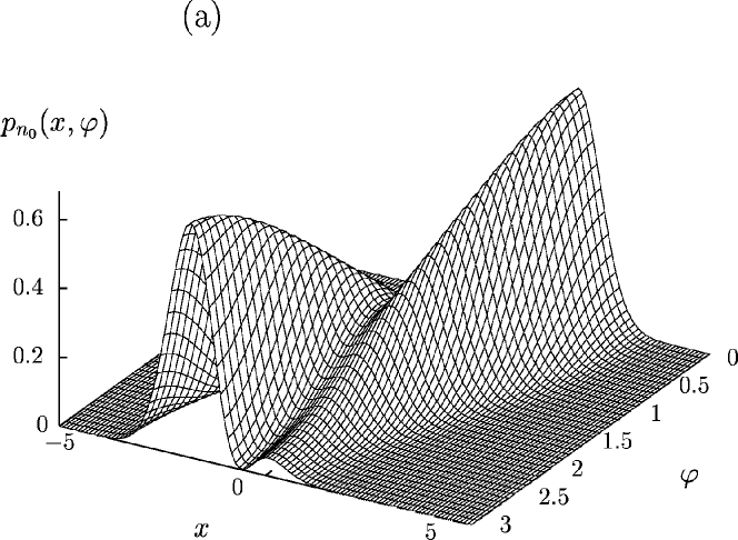
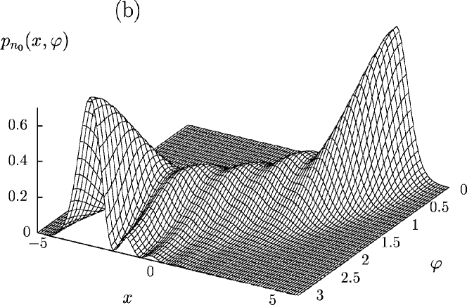
Figure 3: The quadrature-component distribution of photon-added coherent states for $\beta^{\prime}$ $\!=$ $\!0.89$ ($|\beta|$ $\!=$ $\!1$, $|T|^{2}$ $\!=$ $\!0.8$) and two values of $n_{0}$ [ (a) $n_{0}$ $\!=$ $\!1$; (b) $n_{0}$ $\!=$ $\!4$].

where $\varphi_{\beta^{\prime}}=\varphi_{\beta}+\varphi_{T}$. Plots of $p_{n_{0}}(x,\varphi)$ are given in Fig. 3 for $n_{0}$ $\!=$ $\!1$ [$P(n_{0})$ $\!\approx$ $\!30\%$] and $n_{0}$ $\!=$ $\!4$ [$P(n_{0})$ $\!\approx$ $\!0.84\%$]. The $\pi$ periodic narrowing (broadening) of the quadrature-component distribution reveals that photon-added coherent states can be regarded as some kind of squeezed states. Nevertheless, they are in general quite different from the two-photon coherent states [22] widely used in squeezed-light description. It is worth noting that in contrast to the familiar two-photon coherent states the photon-added coherent states are non-Gaussian states. In particular, the variance of $\hat{x}(\varphi)$ is given by [16]

$$(\Delta\hat{x}(\varphi))^{2}=\langle\hat{x}(\varphi)^{2}\rangle-\langle\hat{x}(\varphi)\rangle^{2}$$ (44)

$$\hskip 4.30554pt=\,\frac{1}{2{\rm L}_{n_{0}}(-2|\beta^{\prime}|^{2})^{2}}\bigg{\{}2|\beta^{\prime}|^{2}\big{[}{\rm L}_{n_{0}}^{2}(-|\beta^{\prime}|^{2}){\rm L}_{n_{0}}(-|\beta^{\prime}|^{2})$$

$$\hskip 4.30554pt-\,{\rm L}_{n_{0}}^{1}(-|\beta^{\prime}|^{2})^{2}\big{]}\cos(2(\varphi+\varphi_{\beta^{\prime}}))-2|\beta^{\prime}|^{2}{\rm L}_{n_{0}}^{1}(-|\beta^{\prime}|^{2})^{2}$$

$$\hskip 4.30554pt-\,{\rm L}_{n_{0}}(-|\beta^{\prime}|^{2})^{2}+2(n_{0}+1){\rm L}_{n_{0}}(-|\beta^{\prime}|^{2}){\rm L}_{n_{0}+1}(-|\beta^{\prime}|^{2})\bigg{\}}.$$

With increasing number of added photons, $n_{0}$, the squeezing effect is (for chosen $|\beta|^{\prime}$ $\!>$ $\!0$) enhanced. Needless to say that when $n_{0}$ $\!=$ $\!0$ (i.e., when no photons are added), then the conditional state $|\Psi_{0}\rangle$ simply reduces to the coherent state $|\beta^{\prime}\rangle$. Finally, it should be noted that when the vacuum is mixed with a Fock state and the zero-photon measurement in one of the output channels of the beam splitter is replaced with a measurement of the $Q$ function (in perfect six- or eight-port balanced homodynings), then the conditional states of the other output channel are similar to the photon-added coherent states [6].

3.2 Squeezed vacuum states

Let us now consider a squeezed-vacuum input state

$$|\Phi\rangle=|0\rangle_{\rm s}=\hat{S}(\xi)|0\rangle,$$ (45)

where

$$\hat{S}(\xi)|0\rangle=\exp\!\left\{-\textstyle\frac{1}{2}\left[(\xi\hat{a}^{\dagger})^{2}-\xi^{\ast}\hat{a}^{2}\right]\right\}|0\rangle=(1-|\kappa|^{2})^{1/4}\sum_{n=0}^{\infty}\frac{[(2n)!]^{1/2}}{2^{n}\,n!}\,\kappa^{n}|2n\rangle,$$ (46)

with $\xi$ $\!=$ $\!|\xi|e^{i\varphi_{\xi}}$ and $\kappa$ $\!=$ $\!e^{i\varphi_{\xi}}\tanh|\xi|$. The conditional output states (19) are seen to be photon-added squeezed vacuum states

$$|\Psi_{n_{0}}\rangle=\frac{1}{\sqrt{{\cal N}^{\prime}_{n_{0}}}}(\hat{a}^{\dagger})^{n_{0}}\hat{S}(\xi^{\prime})|0\rangle,$$ (47)

where $\xi^{\prime}$ $\!=$ $\!|\xi^{\prime}|e^{i(\varphi_{\xi}+2\varphi_{T})}$, and $\tanh|\xi^{\prime}|$ $\!=$ $\!|T|^{2}\tanh|\xi|$. In the photon-number basis they read as

$$|\Psi_{n_{0}}\rangle=\frac{(1-|\kappa^{\prime}|^{2})^{1/4}}{\sqrt{{\cal N}^{\prime}_{n_{0}}}}\sum_{n=n_{0}}^{\infty}b_{n,n_{0}}(\kappa^{\prime})\,|n\rangle,$$ (48)

where

$$b_{n,n_{0}}(\kappa^{\prime})=\frac{\sqrt{n!}}{\Gamma\!\left[\frac{1}{2}(n-n_{0})+1\right]}\,{\textstyle\frac{1}{2}\left[1+(-1)^{n-n_{0}}\right]}\left(\textstyle\frac{1}{2}\kappa^{\prime}\right)^{(n-n_{0})/2}$$ (49)

and $\kappa^{\prime}$ $\!=$ $\!T^{2}\kappa$. Note that when $n_{0}$ $\!=$ $\!0$ then $|\Psi_{n_{0}}\rangle$ simply reduces to a squeezed vacuum state (46), with $\kappa^{\prime}$ in place of $\kappa$.

For the sake of tranceparency and without loss of generality we will assume that $\kappa^{\prime}$ is real, i.e., $\!\varphi_{\xi}+2\varphi_{T}$ $\!=$ $\!k\pi$, with $k$ being an integer. Note that the effect of other phases is simply a rotation in phase space. Using the doubling formula for the Gamma-function,

$$\frac{\Gamma(2n)}{\Gamma(n+1/2)}=\frac{4^{n}}{2\sqrt{\pi}}\,\Gamma(n),$$ (50)

and the Gauss-series of the hypergeometric function [25],

$${\rm F}(a,b,c;z)=\frac{\Gamma(c)}{\Gamma(a)\Gamma(b)}\sum_{n=0}^{\infty}\frac{\Gamma(a+n)\Gamma(b+n)}{\Gamma(c+n)}\frac{z^{n}}{n!},$$ (51)

the normalization constant ${\cal N}^{\prime}_{n_{0}}$ can be derived to be

$${\cal N}^{\prime}_{n_{0}}=\sqrt{1\!-\!\kappa^{\prime 2}}\,n_{0}!\,{\rm F}\!\left[\textstyle\frac{1}{2}(n_{0}+1),\textstyle\frac{1}{2}(n_{0}+2),1;\kappa^{\prime 2}\right].$$ (52)

From Eqs. (21) and (46) [together with Eqs. (50) and (51)] the probability of producing photon-added squeezed vacuum states is derived to be

$$P(n_{0})=|R|^{2n_{0}}\sqrt{1\!-\!|\kappa|^{2}}\,{\rm F}\!\left(n_{0}+1,\textstyle\frac{1}{2},1;\kappa^{\prime 2}\right).$$ (53)

Examples of $P(n_{0})$ are plotted in Fig. 4. In particular we see that for not too small transmittance of the beam splitter (and chosen $n_{0}$) the probability $P(n_{0})$ can increase with the value of $|\kappa|$, which is similar to the behavior shown in Fig. 3 for a coherent input state. Note that the mean photon number of the squeezed vacuum (46) is given by $|\kappa|^{2}/(1-|\kappa|^{2})$.

Using Eq. (48), the photon-number distribution

$$p_{n_{0}}(n)=|\langle\,n|\Psi_{n_{0}}\rangle|^{2}$$ (54)

of the photon-added squeezed vacuum states can be given by

$$p_{n_{0}}(n)=\frac{1}{{\cal N}^{\prime\prime}_{n_{0}}}\left|b_{n,n_{0}}(\kappa^{\prime})\right|^{2}\quad{\rm if}\quad n\geq n_{0}$$ (55)

and $p_{n_{0}}(n)$ $\!=$ $\!0$ elsewhere, and

$${\cal N}^{\prime\prime}_{n_{0}}=n_{0}!\,{\rm F}\!\left[\textstyle\frac{1}{2}(n_{0}+1),\textstyle\frac{1}{2}(n_{0}+2),1;\kappa^{\prime 2}\right].$$ (56)

From Eqs. (55) and (49) we easily see that when the number of the added photons, $n_{0}$, is even (odd), then the photon-number distribution is nonzero only for even (odd) photon numbers. This oscillating behavior of the photon-number distribution obviously reflects the fact that only even photon numbers contribute to the squeezed vacuum state to which photons are added. In particular the mean photon number

$$\langle\hat{n}\rangle=\sum_{n}n\,p_{n_{0}}(n)$$ (57)

may be rewritten as

$$\langle\hat{n}\rangle=\kappa^{\prime}\frac{\partial}{\partial\kappa^{\prime}}\log\!\left[\kappa^{\prime n_{0}}{\cal N}^{\prime\prime}_{n_{0}}\right].$$ (58)

Using standard formulas for the derivative of the hypergeometric function [25], we find that

$$\langle\hat{n}\rangle=n_{0}+{\textstyle\frac{1}{2}}\kappa^{\prime 2}(n_{0}+1)(n_{0}+2)\,\frac{{\rm F}\!\left[\frac{1}{2}(n_{0}+3),\frac{1}{2}(n_{0}+4),2;\kappa^{\prime 2}\right]}{{\rm F}\!\left[\frac{1}{2}(n_{0}+1),\frac{1}{2}(n_{0}+2),1;\kappa^{\prime 2}\right]}\,.$$ (59)

As expected, for $\kappa^{\prime}$ $\!\to$ $\!0$ $\langle\hat{n}\rangle$ approaches $n_{0}$ and it increases with $\kappa^{\prime}$ and $n_{0}$. Examples of the photon-number distribution are shown in Fig. 5 for $n_{0}$ $\!=$ $\!1$ [$P(n_{0})$ $\!\approx$ $\!23\%$] and $n_{0}$ $\!=$ $\!4$ [$P(n_{0})$ $\!\approx$ $\!0.45\%$].

Let us now turn to the quadrature-component distribution. Combining Eqs. (39), (41), and (48), we derive

$$p_{n_{0}}(x,\varphi)=\frac{2^{-n_{0}}}{{\cal N}^{\prime\prime}_{n_{0}}\sqrt{\pi\Delta^{n_{0}+1}}}\,\exp\!\left(-\frac{1-\kappa^{\prime 2}}{\Delta}\,x^{2}\right)\left|{\rm H}_{n_{0}}\!\left[\sqrt{(1-\kappa^{\prime}e^{i2\varphi})/\Delta}\,x\right]\right|^{2},$$ (60)

where

$$\Delta=1+\kappa^{\prime 2}-2\kappa^{\prime}\cos(2\varphi).$$ (61)

Note that in the derivation of Eq. (60) the summation formula [21]

$$\sum_{k=0}^{\infty}\frac{z^{k}}{k!}\,{\rm H}_{2k+n}(x)=(1+4z)^{-n/2-1/2}$$ (62)

$$\hskip 8.61108pt\times\,\exp\!\left(\frac{4zx^{2}}{1+4z}\right){\rm H}_{n}\!\left(\frac{x}{\sqrt{1+4z}}\right)\quad\left(|z|<\textstyle\frac{1}{2}\right)$$

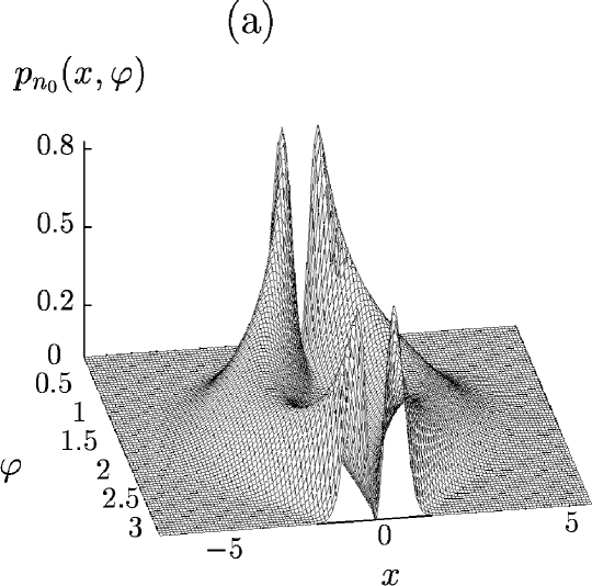
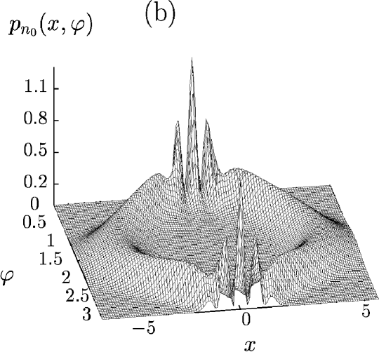
Figure 6: The quadrature-component distribution of photon-added squeezed vacuum states for $\kappa^{\prime}$ $\!=$ $\!0.6$ ($|\kappa|$ $\!=$ $\!0.67$, $|T|^{2}$ $\!=$ $\!0.8$) and two values of $n_{0}$ [(a) $n_{0}$ $\!=$ $\!1$; (b) $n_{0}$ $\!=$ $\!4$].

has been used. The quadrature-component distributions plotted in Fig. 6 correspond to the same parameters as in Fig. 5. From inspection of Fig. 6, interference fringes for $\varphi$ close to $0$ or $\pi$ are seen, whereas for $\varphi$ near $\pi/2$ two separated peaks are observed. The behavior is typical of a Schrödinger-cat-like superposition of two macroscopically distinguishable states.

Next let us calculate the Wigner function

$$W_{n_{0}}(x,p)=\frac{1}{\pi}\int\limits_{-\infty}^{+\infty}{d}y\,e^{2ipy}\langle x\!-\!y|\Psi_{n_{0}}\rangle\langle\Psi_{n_{0}}|x\!+\!y\rangle.$$ (63)

Using Eqs. (41) and (48) [together with Eq. (62)], after some calculation we obtain

$$W_{n_{0}}(x,p)=\frac{2e^{-\lambda x^{2}}}{\pi^{3/2}{\cal N}^{\prime\prime}_{n_{0}}[2(\kappa^{\prime}+1)]^{n_{0}+1}}$$ (64)

$$\hskip 34.44434pt\times\int\limits_{-\infty}^{+\infty}{d}ye^{-\lambda y^{2}+2ipy}\,{\rm H}_{n_{0}}\!\left(\frac{x\!-\!y}{\sqrt{1\!+\!\kappa^{\prime}}}\right){\rm H}_{n_{0}}\!\left(\frac{x\!+\!y}{\sqrt{1\!+\!\kappa^{\prime}}}\right),$$

where

$$\lambda=\frac{1-\kappa^{\prime}}{1+\kappa^{\prime}}\,.$$ (65)

Performing the $y$ integration [21] yields

$$W_{n_{0}}(x,p)=\!\frac{|\kappa^{\prime}|^{n_{0}}\sqrt{2}}{\pi{\cal N}^{\prime\prime}_{n_{0}}[2(1\!-\!\kappa^{\prime 2})]^{n_{0}+1/2}}\exp\!\left(\!-\lambda x^{2}\!-\!\frac{p^{2}}{\lambda}\!\right)$$ (66)

$$\hskip 34.44434pt\times\sum_{k=0}^{n_{0}}\!{n_{0}\choose k}^{2}\!k!\!\left(\frac{-2}{|\kappa^{\prime}|}\right)^{k}\left|{\rm H}_{n_{0}-k}\!\left[i\sqrt{\frac{\lambda}{\kappa^{\prime}}}\left(x\!+\!i\frac{p}{\lambda}\right)\right]\right|^{2}\!\!.$$

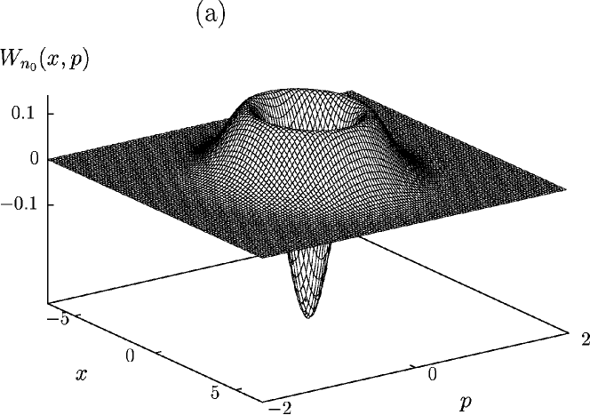
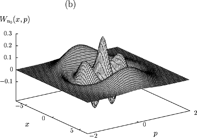
Figure 7: The Wigner function of photon-added squeezed vacuum states for $\kappa^{\prime}$ $\!=$ $\!0.6$ ($|\kappa|$ $\!=$ $\!0.67$, $|T|^{2}$ $\!=$ $\!0.8$) and two values of $n_{0}$ [(a) $n_{0}$ $\!=$ $\!1$; (b) $n_{0}$ $\!=$ $\!4$].

The Wigner functions in Fig. 7 are plotted for the same parameters as in Figs. 5 and 6. We again recognize the typical features of Schrödinger-cat-like states.

Finally, let us consider the Husimi function

$$Q_{n_{0}}(x,p)=\frac{1}{2\pi}\,|\langle\alpha|\Psi_{n_{0}}\rangle|^{2},$$ (67)

where $|\alpha\rangle$ is a coherent state and $\alpha$ $\!=$ $\!2^{-1/2}(x\!+\!ip)$. Recalling the expansion of the coherent states in the Fock basis, Eq. (30), and using Eq. (48), we easily find that

$$Q_{n_{0}}(x,p)=\frac{(x^{2}+y^{2})^{n_{0}}}{\pi 2^{n_{0}+1}{\cal N}^{\prime\prime}_{n_{0}}}\,\exp\!\left\{-\textstyle\frac{1}{2}\left[(1-\kappa^{\prime})x^{2}+(1+\kappa^{\prime})p^{2}\right]\right\}.$$ (68)

Note that the Husimi function is a phase-space function that can be measured in multiport balanced homodyning, such as six-port [26] or eight-port [27] detections. Since the Husimi function can be regarded as a smoothed Wigner function, the oscillating behavior and the negative values that are typical of the Wigner function (see Fig. 7) cannot be observed.

Schrödinger cat-like states are commonly defined as superpositions of two macroscopically distinguishable states. From Eqs. (48) and (49) it is seen that $|\Psi_{n_{0}}\rangle$ can be given by the superposition

$$|\Psi_{n_{0}}\rangle=A\left(|\Psi^{(+)}_{n_{0}}\rangle+|\Psi^{(-)}_{n_{0}}\rangle\right),$$ (69)

where

$$|\Psi^{(\pm)}_{n_{0}}\rangle=\frac{1}{\sqrt{{{\cal N}^{\prime\prime(\pm)}_{n_{0}}}}}\sum_{n=n_{0}}^{\infty}b^{(\pm)}_{n,n_{0}}(\kappa^{\prime})\,|n\rangle,$$ (70)

with

$$b^{(\pm)}_{n,n_{0}}(\kappa^{\prime})=\frac{\sqrt{n!}}{\Gamma[(n-n_{0})/2+1]}\left(\pm\sqrt{\textstyle\frac{1}{2}\kappa^{\prime}}\right)^{n-n_{0}}\!\!\!.$$ (71)

Using standard relations [25], the normalization factor ${{\cal N}^{\prime\prime(\pm)}_{n_{0}}}$ in Eq. (70) can be expressed in terms of derivatives of the hypergeometric function,

$${{\cal N}^{\prime\prime(\pm)}_{n_{0}}}=\frac{\partial^{n_{0}}}{\partial{\kappa^{\prime}}^{n_{0}}}{\kappa^{\prime}}^{n_{0}}\bigg{\{}{\rm F}\!\left(\textstyle\frac{1}{2},1,1;\kappa^{\prime 2}\right)+\frac{2}{\pi}\kappa^{\prime}{\rm F}\!\left(1,1,\textstyle\frac{3}{2};\kappa^{\prime 2}\right)\bigg{\}}\,,$$ (72)

and the normalization constant in Eq. (69) is given by $A$ $\!=$ $\!\frac{1}{2}({{\cal N}^{\prime\prime(\pm)}_{n_{0}}}/{\cal N}^{\prime\prime}_{n_{0}})^{1/2}$.

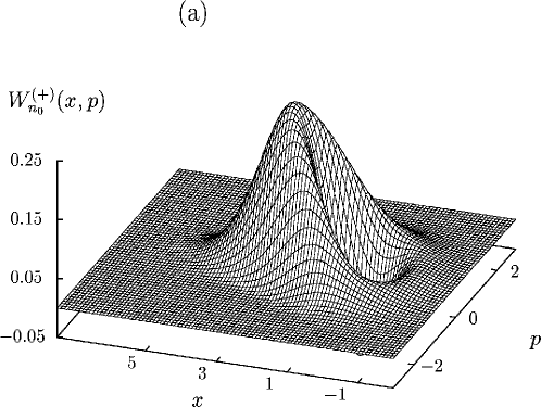
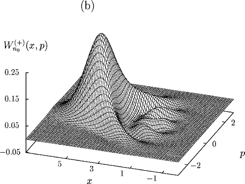
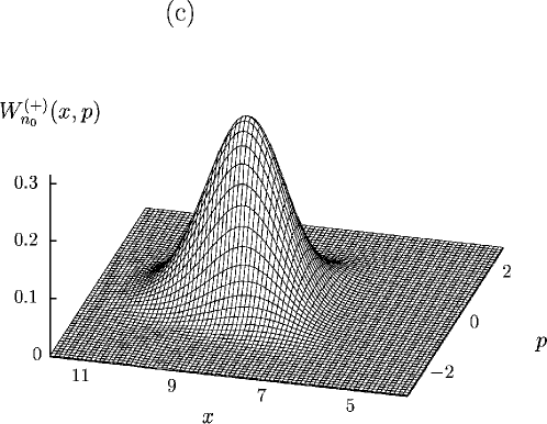
Figure 8: The Wigner function of the component states $|\Psi_{n_{0}}^{(+)}\rangle$ for $\kappa^{\prime}$ $\!=$ $\!0.6$ ($|\kappa|$ $\!=$ $\!0.67$, $|T|^{2}$ $\!=$ $\!0.8$) and three values of $n_{0}$ [(a) $n_{0}$ $\!=$ $\!1$; (b) $n_{0}$ $\!=$ $\!4$; (c) $n_{0}$ $\!=$ $\!15$].

To demonstrate the nonclassical properties of the component states $|\Psi^{(\pm)}_{n_{0}}\rangle$, in Fig. 8 we have plotted the Wigner function $W_{n0}^{(+)}(x,p)$ of $|\Psi^{(+)}_{n_{0}}\rangle$ for various values of $n_{0}$. We see that with increasing $n_{0}$ the Wigner function becomes less structurized and the negative values are more and more suppressed [e.g., for $\kappa^{\prime}$ $\!=$ $\!0.6$ and $n_{0}$ $\!=$ $\!15$ the Wigner function attains negative values of the order of magnitude of $-10^{-4}$, Fig. 8(c)]. It is worth noting that the component states $|\Psi^{(\pm)}_{n_{0}}\rangle$ can be regarded as non-Gaussian squeezed coherent states that tend to the familiar Gaussian squeezed coherent states as $n_{0}$ becomes sufficiently large. To illustrate the difference between the states $|\Psi^{(\pm)}_{n_{0}}\rangle$ and the Gaussian squeezed coherent states, let us consider the Husimi function $Q_{n_{0}}^{(\pm)}(x,p)$ $\!=$ $\!|\langle\alpha|\Psi_{n_{0}}^{(\pm)}\rangle|^{2}$, with $\alpha$ $\!=$ $\!2^{-1/2}(x\!+\!ip)$. Using the expansions (30) and (70), we derive

$$Q_{n_{0}}^{(\pm)}(x,p)=\frac{|\alpha|^{2n_{0}}e^{-|\alpha|^{2}}}{2\pi{{\cal N}^{\prime\prime}_{n_{0}}}^{(\pm)}}\,\exp\!\left[{\textstyle\frac{1}{2}}\kappa^{\prime}\left(\alpha^{2}+{\alpha^{\ast}}^{2}\right)\right]\left|{\rm Erfc}\!\left(\mp\sqrt{\textstyle\frac{1}{2}\kappa^{\prime}}\alpha\right)\right|^{2}.$$ (73)

Here, the relation [28]

$$\sum_{n=0}^{\infty}\frac{z^{n}}{\Gamma(\frac{1}{2}n+1)}=\exp(z^{2})\,{\rm Erfc}(-z)$$ (74)

has been used, where ${\rm Erfc}(z)$ is the complementary complex error function defined by

$${\rm Erfc}(z)=1-{\rm Erf}(z)=\frac{2}{\sqrt{\pi}}\int_{z}^{\infty}{d}z\,e^{-t^{2}}.$$ (75)

From Eq. (73) the asymptotic form of $Q_{n_{0}}^{(\pm)}(x,p)$ for large $n_{0}$ is derived to be (see Appendix A)

$$Q_{n_{0}}^{(\pm)}(x,p)\approx\frac{n_{0}!}{4\pi^{2}\!n_{0}{{\cal N}^{\prime\prime}_{n_{0}}}^{(\pm)}}\,\exp(-|\alpha\mp\sqrt{n_{0}}|^{2})\exp\!\left[{\textstyle\frac{1}{2}\kappa^{\prime}}\left(\alpha^{2}+{\alpha^{\ast}}^{2}\right)\right].$$ (76)

From inspection of Eq. (76) we see that for large $n_{0}$ the Husimi function $Q_{n_{0}}^{(\pm)}(x,p)$ becomes a single-peaked Gaussian centered at $\pm\sqrt{n_{0}}$, i.e., when $n_{0}$ $\!\to$ $\!\infty$ then the states $|\Psi_{n_{0}}^{(\pm)}\rangle$ tend to the familiar Gaussian squeezed coherent states.

4 Mixed photon-added states

So far we have assumed that a mode prepared in a photon-number state $|n_{0}\rangle$ is fed into one of the input ports of a beam splitter, so that exactly $n_{0}$ photons can be added to the state of the (signal) mode fed into the other input port. In practice however, it may be more realistic to consider a statistical mixture of photon-number states rather than a pure state, because of smoothings in the generation of photon-number states [20]. It is worth noting that – apart from some smearing – the above given results remain valid as long as the statistical mixture of photon-number states is sub-Poissonian. Let us return to Eq. (11) and assume that

$$\hat{\varrho}_{\rm in}(n_{0})=\hat{\varrho}_{{\rm in}1}\otimes\hat{\varrho}_{{\rm in}2},$$ (77)

where

$$\hat{\varrho}_{{\rm in}2}=\sum_{n_{0}}\tilde{p}_{n_{0}}\,|n_{0}\rangle\langle n_{0}|\,.$$ (78)

To be more specific, let us consider (as an example of a sub-Poissonian distribution) a binomial probability distribution,

$$\tilde{p}_{n_{0}}={N\choose n_{0}}p^{n_{0}}(1-p)^{N-n_{0}}\quad{\rm if}\quad n_{0}\leq N$$ (79)

and $\tilde{p}_{n_{0}}$ $\!=$ $\!0$ elsewhere ($0$ $\!<$ $\!p$ $\!<$ $\!1$). Note that for $p$ $\!\to$ $\!0$, $N$ $\!\to$ $\!\infty$, and $pN$ finite, the binomial distribution (79) reduces to a Poisson distribution, with $\bar{n}$ $\!=$ $\!pN$ being the mean photon number. Using Eqs. (77) and (78), in place of Eq. (18) we easily find that detection of no photons in one of the output channels of the beam splitter now yields the conditional (mixed photon-added) state

$$\hat{\varrho}_{{\rm out}1}(m_{2}=0)=\sum_{n_{0}}\tilde{p}_{n_{0}}\,\hat{\varrho}_{{\rm out}1}(n_{0},m_{2}=0)=\sum_{n_{0},\Phi}\tilde{p}_{n_{0}}\tilde{p}_{\Phi}|\,\Psi_{n_{0}}\rangle\big{\langle}\Psi_{n_{0}}|$$ (80)

in the other output channel. Accordingly, the probability of detecting the state is the average of $P(n_{0})$ given in Eq. (21),

$$P=\sum_{n_{0}}\tilde{p}_{n_{0}}P(n_{0}).$$ (81)

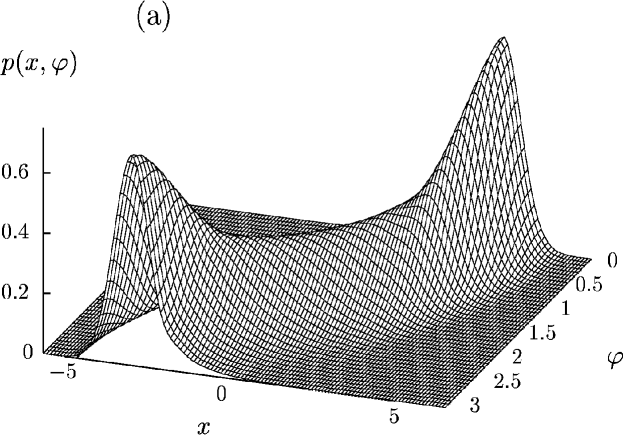
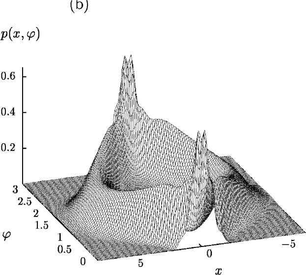
Figure 9: The quadrature-component distributions of mixed photon-added coherent (a) and squeezed vacuum (b) states for $p$ $\!=$ $\!0.8$ and $N$ $\!=$ $\!5$ in Eq. (79), the values of the other parameters being the same as in Figs. 3 and 6.

Examples of the quadrature-component distributions $p(x,\varphi)$ $\!=$ $\!\sum_{n_{0}}\tilde{p}_{n_{0}}\,p_{n_{0}}(x,\varphi)$ of mixed photon-added coherent and squeezed vacuum states are plotted in Figs. 9(a) and (b), respectively. In the figures it is assumed that $p$ $\!=$ $\!0.8$ and $N$ $\!=$ $\!5$ [i.e., the mean photon number and the photon-number variance are $\bar{n}$ $\!=$ $\!4$ and $\overline{(\Delta n)^{2}}$ $\!=$ $\!0.8$, respectively]. Comparing Figs. 9(a) and (b) with Figs. 3(b) and 6(b), respectively, we see that the typical nonclassical features (such as squeezing and quantum interference) are preserved, even when the photon number state $|n_{0}\rangle$ is replaced with a sub-Poissonian mixed state (78) (i.e., a smeared photon-number state). As expected, the probabilities (81) of observing the mixed photon-added states become smaller than those obtained for pure Fock-state inputs [$P\approx\!0.07\%$ for the mixed photon-added coherent state in Fig. 9(a) and $P\approx\!0.04\%$ for the mixed photon-added squeezed vacuum state in Fig. 9(b)].

5 Conclusion

We have studied the problem of generating photon-added states using conditional output measurement on a beam splitter. When a single-mode radiation field is mixed with a mode prepared in a photon-number number state, then the mode in one of the output channels photon-added is prepared in a photon-added state, provided that in the other output channel no photons are detected. We have studied the conditions under which the photon-added states can be regarded as photon-added input states or states that belong the same class of states as the photon-added input states do. Typical examples of input states to which photons can be added in this way are thermal states, coherent states, squeezed states, displaced photon-number states, and coherent phase states.

Photon-added states are highly nonclassical states in general. In particular, photon-added coherent states can be regarded as non-Gaussian squeezed states, as can be seen, e.g., from the derived expression for the quadrature-component distribution. Another interesting class of states that can be produced in the way described are photon-added squeezed vacuum states, which exhibit all the typical properties of Schrödinger-cat-like states. Photon adding to a squeezed vacuum can therefore be regarded as a method for producing Schrödinger-cats. We have analyzed the photon-added squeezed vacuum states in terms of the photon-number and the quadrature-component distributions and phase-space functions, such as the Wigner and Husimi functions, and have presented both analytical and numerical results. We have shown that photon-added squeezed vacuum states may be regarded as superpositions of two non-Gaussian squeezed coherent states that tend to the familiar (Gaussian) squeezed coherent states as the number of added photons goes to infinity.

With regard to possible experimental implementations, we have also performed calculations allowing for an input mode prepared in a statistical mixture of Fock states in place of a pure Fock state. As expected, mixtures of Fock states give rise to conditional states that can be regarded, in a sense, as smeared photon-added states. It is worth noting that when the photon-number distribution of the mixtures is typically sub-Poissonian, then the characteristic nonclassical features of photon-added states can be observed. In the paper we have demonstrated the effect of smearing assuming a binomial photon-number distribution. In particular, combining mixed Fock states of that type with a squeezed vacuum, the conditional output states also exhibit, in general, properties that are typically observed for Schrödinger-cat-like states. That is to say, the characteristic properties of squeezed vacuum states are (apart of some smearing) preserved. Clearly, when the photon-number distribution of the mixed Fock states becomes Poissonian, then the nonclassical properties that are typically associated with photon-added states disappear.

Appendix Appendix A Derivation of Eq. (76)

To find the asymtotoic form (76) of $Q_{n_{0}}^{(\pm)}(x,p)$ defined in Eq. (73), we first consider the asymptotic behavior of $|\alpha|^{2n_{0}}e^{-|\alpha|^{2}}$ for $n_{0}$ $\!\to$ $\!\infty$,

$$|\alpha|^{2n_{0}}e^{-|\alpha|^{2}} \approx \!\frac{n_{0}!}{2\pi\!n_{0}}\,\exp\!\left(-\frac{|\alpha^{2}-n_{0}|^{2}}{2n_{0}}\right)$$ (A 1)

$$= \frac{n_{0}!}{2\pi\!n_{0}}\,\exp\!\left(-\frac{|\alpha+\sqrt{n_{0}}|^{2}\;|\alpha-\sqrt{n_{0}}|^{2}}{2n_{0}}\right),$$

which may be approximated by the sum of two Gaussians centered at $\alpha$ $\!=$ $\!\pm\sqrt{n_{0}}$,

$$|\alpha|^{2n_{0}}e^{-|\alpha|^{2}}\approx\frac{n_{0}!}{2\pi\!n_{0}}\,\left[\exp\!\left(-|\alpha\!-\!\sqrt{n_{0}}|^{2}\right)+\exp\!\left(-|\alpha\!+\!\sqrt{n_{0}}|^{2}\right)\right].$$ (A 2)

Next let us consider the infinite-series approximation of the complementary complex error function [28],

$${\rm Erfc}(x+iy)\approx{\rm Erfc}(x)+\frac{e^{-x^{2}}}{2\pi x}\left[1-\cos(2xy)+i\sin(2xy)\right]$$ (A 3)

$$\hskip 51.6665pt+\,\frac{2e^{-x^{2}}}{\pi}\sum_{n=1}^{\infty}\frac{e^{-n^{2}/4}}{n^{2}+4x^{2}}\left[f_{n}(x,y)+ig_{n}(x,y)\right],$$

where $f_{n}(x,y)$ and $g_{n}(x,y)$ are given by

$$f_{n}(x,y)=2x[1-\cosh(ny)\cos(2x)]+n\sinh(ny)\sin(2xy)$$

and

$$g_{n}(x,y)=2x\cosh(ny)\sin(2x)+n\sinh(ny)\cos(2xy).$$ (A 4)

From Eq. (A 3) [together with Eqs. (Appendix A) and (A 4)] we easily see that

$${\rm Erfc(x+iy)}\approx{\rm Erfc(x)}\quad{\rm if}\quad|x|\gg 1.$$ (A 5)

Further the approximations

$${\rm Erfc}(x) \approx 0\quad{\rm if}\quad x\gg 1,$$ (A 6)

$${\rm Erfc}(-x) \approx 0\quad{\rm if}\quad x\ll-1.$$ (A 7)

are valid [28]. Recalling Eq. (73), we see that the argument $x\!+\!iy$ in Eq. (A 3) corresponds to $\mp\sqrt{\textstyle\frac{1}{2}\kappa^{\prime}}\alpha$. Since for chosen $\kappa^{\prime}$ ($\kappa^{\prime}$ $\!\neq$ $\!0$) and sufficiently large $n_{0}$ the Gaussians in Eq. (A 2) are nonzero only for large $|\alpha|$, we can apply the approximations (A 5) – (A 7), which [together with Eq. (A 2)] yields the asymptotic form (76). Note that due to the error function only one of the two Gaussians in Eq. (A 2) survives.

Figure 1: Scheme of the experimental setup. When a signal mode prepared in a state $\hat{\varrho}_{{\rm in}1}$ is mixed with another input mode prepared in a Fock state $|n_{0}\rangle$ and in one of the output channels of the beam splitter no photons are recorded by a detector (D), then the quantum state $\hat{\varrho}_{{\rm out}1}$ of the mode in the other output channel “collapses” to a photon-added state.

Figure 2: The probability of producing photon-added coherent states is shown as a function of $|\beta|$ for two values of the beam-splitter transmittance [(a) $|T|^{2}$ $\!=$ $\!0.3$; (b) $|T|^{2}$ $\!=$ $\!0.8$] and various values of $n_{0}$.

Figure 4: The probability of producing photon-added squeezed vacuum states is shown as a function of $|\kappa|$ for two values of the beam-splitter transmittance [(a) $|T|^{2}$ $\!=$ $\!0.3$; (b) $|T|^{2}$ $\!=$ $\!0.8$] and various values of $n_{0}$.

Figure 5: The photon-number distribution of photon-added squeezed vacuum states for $\kappa^{\prime}$ $\!=$ $\!0.6$ ($|\kappa|$ $\!=$ $\!0.67$, $|T|^{2}$ $\!=$ $\!0.8$) and two values of $n_{0}$ ($n_{0}$ $\!=$ $\!1$, full bars; $n_{0}$ $\!=$ $\!4$, dashed bars).

References

- [1] J.von Neumann, Mathematical Foundations of Quantum Mechanics (Princeton University Press, Princeton, N.J.,1955).
- [2] K. Watanabe and Y. Yamamoto, Phys. Rev. A 38, 3556 (1988).
- [3] S. Song, C.M. Caves, and B. Yurke, Phys. Rev. A 41, 5261 (1990); B. Yurke, W. Schleich, and D.F. Walls, Phys. Rev. A 42, 1703 (1990).
- [4] M. Ban, Phys. Rev. A 49, 5078 (1994).
- [5] M. Ban, Opt. Commun. 130, 365 (1996).
- [6] M. Ban, J. Mod. Opt. 43, 1281 (1996).
- [7] M Brune, S. Haroche, S. Lefèvre, J.M. Raimond, and N. Zagury, Phys. Rev. Lett. 65, 976 (1990); M Brune, S. Haroche, S. J.M. Raimond, L. Davidovich, and N. Zagury, Phys. Rev. 45, 5193 (1992); K. Vogel, V.M. Akulin, and W.P. Schleich, Phys. Rev. Lett. 71, 1816 (1993).
- [8] J.I. Cirac, R. Blatt, A. S. Parkins, and P. Zoller, Phys. Rev. Lett. 70, 762 (1993); R.L. de Matos Filho and W. Vogel, Phys. Rev. Lett. 76, 4520 (1996).
- [9] M. Ueda, Phys. Rev. A 41, 3875 (1990); M. Ueda, N. Imoto , and T. Ogawa, Phys. Rev. A 41, 3891 (1990); M. Ueda and M. Kitagawa, Phys. Rev. Lett. 68, 3424 (1992).
- [10] M. Ueda, N. Imoto, H. Nagoaka, and T. Ogawa, Phys. Rev. A 46, 2859 (1992);
- [11] T. Ogawa, M. Ueda, N. Imoto, Phys. Rev. A 43, 6458 (1991);
- [12] G. J. Milburn and D. F. Walls, Phys. Rev. A 30, 56 (1984); H. P. Yuen, Phys. Rev. Lett. 56, 2176 (1985); A. S. Parkins, P. Marte, P. Zoller, and H. J. Kimble, Phys. Rev. Lett. 71, 3095 (1993); M. J. Holland, D. F. Walls, and P. Zoller, Phys. Rev. Lett. 67, 1716 (1991);
- [13] H. Paul, P. Törmä, T. Kiss, and I. Jex, Journal of Optics and Fine Mechanics, to be published.
- [14] M. Dakna, T. Anhut, T. Opatrný. L. Knöll, and D.–G. Welsch, Phys. Rev. A (to be published).
- [15] G. Björk and Y. Yamamoto, Phys. Rev. A 37, 4229 (1987).
- [16] G. S. Agarwal and K. Tara, Phys. Rev. A 43, 492 (1991).
- [17] B. Yurke, S.L. McCall, and J.R. Klauder, Phys. Rev. A 33, 4033 (1986).
- [18] R.A. Campos, B.E.A. Saleh, and M.C. Teich, Phys. Rev. A 40, 1371 (1989).
- [19] R.M. Wilcox, J. Math. Phys. 8, 962 (1967).
- [20] L. Davidovich, Rev. mod. phys. 68, 127 (1996).
- [21] A. P. Prudnikov, Yu. A. Brychkov and O. J Marichev, Integral and Series, Vol 2 (Gordon and Breach, New Yok, 1986).
- [22] H. P. Yuen, Phys. Rev. A 13, 2226 (1976).
- [23] R. Nath and S. K. Muthu, Quantum Semiclass. Opt. 8, 915 (1996).
- [24] W. Vogel and D.-G. Welsch, Lectures on Quantum Optics (Akademie Verlag, Berlin, 1994).
- [25] A. Erdelyi, Higher Transcendental Functions, Batman Manuscript Project, Vol 2 (McGraw-Hill, New York, 1953).
- [26] N.G. Walker, J. Mod. Opt. 34, 15 (1987); A. Zucchetti, W. Vogel, and D.-G. Welsch, Phys. Rev. A 54, 856 (1996); M.G.A. Paris, A.V. Chizhov, and O. Steuernagel, Opt. Commun. 134, 117 (1997).
- [27] N.G. Walker and J.E. Caroll, Electron. Lett. 20, 981 (1984); M. Freyberger, K. Vogel, and W.P. Schleich, Phys. Lett. A 176, 41 (1993).
- [28] M. Abramowitz and I. A. Stegun, Hanbook of Mathematical Functions (harry Deutsch, 1984).