Least-squares inversion for density-matrix reconstruction

Abstract

We propose a method for reconstruction of the density matrix from measurable time-dependent (probability) distributions of physical quantities. The applicability of the method based on least-squares inversion is – compared with other methods – very universal. It can be used to reconstruct quantum states of various systems, such as harmonic and and anharmonic oscillators including molecular vibrations in vibronic transitions and damped motion. It also enables one to take into account various specific features of experiments, such as limited sets of data and data smearing owing to limited resolution. To illustrate the method, we consider a Morse oscillator and give a comparison with other state-reconstruction methods suggested recently.

I Introduction

During the last years the problem of quantum-state measurement has been of increasing interest. Advances in the experimental techniques, which have allowed the physicists to measure not only single observables of a quantum-mechanical system but – for certain systems – the quantum state as a whole, have stimulated both experimental and theoretical research. A number of proposals for measuring quantum states have been made and various quantum-mechanical systems have been considered.

In quantum optics balanced homodyning has been a very fruitful method for tomographical reconstruction [2] of the quantum state of optical fields. Measuring the quadrature-component statistics and using inverse Radon transform techniques, the method was successfully applied to the determination of the Wigner function of single-mode signal fields [3]. The method (also called optical homodyne tomography) has also been extended to direct sampling of the density matrix in a quadrature-component basis [4] and in the Fock basis [5, 6]. Tomographical methods can also be used for reconstructing the quantum state of matter systems, such as molecular vibrations [7] or the transverse motion of an atom beam [8]. In the case of molecular vibrations the time- and frequency-resolved fluorescence spectrum of the molecule plays the role of the quadrature components, provided that the vibrational frequencies in the two electronic states are almost equal to each other and the vibrational motion is approximately harmonic. Further, tomographical methods have been considered in the reconstruction of the (harmonic) center-of-mass motion of trapped atoms [9].

Including in the balanced detection scheme additional vacuum inputs, the quantum state of optical fields can be directly measured in terms of phase-space functions [10]. Using unbalanced homodyning, the displaced photon-number statistics of the signal field can be measured, from which the quantum state can be obtained in terms of phase-space functions [11] and the density matrix in the Fock basis [12]. The method also applies to matter systems and was used to reconstruct the quantum state of the (harmonic) center-of mass motion of trapped ions [13]. In this case the coherent displacements are induced by rf fields that are resonant to the motional frequency.

The methods considered so far are restricted to undamped harmonic oscillators. However, in many physical systems anharmonic motions (modified by dampings) are observed. Recently, interesting nonclassical quantum states have been prepared in systems that are typically anharmonic. Examples are the generation of amplitude-squeezed states in molecules [7, 14] and of Schrödinger cat-like states in atomic Rydberg wave packets [15]. A first attempt has been made to reconstruct the quantum state of anharmonic molecular vibrations using time-resolved fluorescence spectroscopy [16]. It has been shown that the density matrix can be obtained by inversion of high-dimensional systems of linear equations. An approach has been given in [17], extending the pattern-function formalism to more general than harmonic potentials and reconstructing the density matrix from the time-dependent position distribution. However, the quantities that are typically measured in molecular spectroscopy are different from position distributions in general. For example, the time-gated fluorescence spectrum measured in experiments of the type described in [7] is determined by the Franck-Condon overlap factors of the vibrational wave functions in two electronic states. For anharmonic vibrations this spectrum cannot be identified with distributions of the type of position distributions and therefore it should be used directly in order to reconstruct the density matrix [18].

In any case there have been a number of open questions, such as those of the determination of suitable sampling functions mapping the measured data onto the density matrix, the choice of optimum observational times, and the inclusion into the scheme of damping effects and data smearing. The aim of the present paper is to offer possible answers to some of them. For all the systems mentioned the general problem to be solved is the inversion of linear equations that relate the measured quantities to the density-matrix elements of the system under study. This can be done in a very effective way using the least-squares method, which dates back to the eras of Legendre and Gauss [19]. Actually, the method has been used in the context of quantum-state reconstruction problems, such as the reconstruction of the quantum state of cavity fields by quantum-state endoscopy [20], vibrations of trapped ions [13], and optical field by balanced [21] and unbalanced [12] homodyning.

For comparison with previous work [17, 22], we will restrict attention to the reconstruction of the density matrix from the time-dependent position distribution of a particle moving in an anharmonic potential. We show that the least-squares method can advantageously be used in order to reduce the statistical error. We further show that the flexibility of the method enables us to perform the reconstruction from data recorded during shorter time intervals and to take into account typical experimental features, such as smeared and imperfect data. Finally, the method can also be used to reconstruct quantum states of damped systems. It is worth noting that the applicability of the method only requires that there are measurable quantities that are linear combinations of all the relevant density-matrix elements of the quantum state of the system under study.

The paper is organized as follows. In Sec. II the problem of construction of sampling functions is considered. Sections III and IV, respectively, are devoted to the questions of observational time and data smearing. Concluding remarks are given in Sec. V. Elements of the least-squares method and the statistical-error analysis are outlined in Apps. A and B.

II Sampling functions

Let us consider a quantum-mechanical system and assume that at some initial time it is prepared in a state with density matrix $\varrho_{n,n^{\prime}}$ $\!=$ $\!\langle n|\hat{\varrho}|n^{\prime}\rangle$, where $|n\rangle$ are the energy eigenstates of the system Hamiltonian. Further, let us assume that there is a measurable time-dependent (probability) distribution $p(x,t)$ of a quantity $x$ that can be given by a linear combination of all density-matrix elements $\varrho_{n,n^{\prime}}$ that are initially excited, with linearly independent coefficient functions $S_{n,n^{\prime}}(x,t)$,

$$p(x,t)=\sum_{n,n^{\prime}}S_{n,n^{\prime}}(x,t)\,\varrho_{n,n^{\prime}}.$$ (1)

When we consider, e.g., a particle that moves in a potential well and is initially prepared in a bound state (e.g., a molecular vibration in a vibronic system below the dissociation level), only the discrete part of the energy spectrum is excited ($n$ $\!=$ $\!1,2,3,\ldots$). For the sake of transparency, in what follows we restrict attention to discrete spectra. However, replacing in Eq. (1) the sums with integrals (or combinations of sums and integrals), excitations of continuous parts of the spectrum can be treated accordingly. For any physical state the density-matrix elements $\varrho_{n,n^{\prime}}$ must eventually decrease indefinitely with increasing $n(n^{\prime})$. Therefore it follows that the expression on the right-hand side of Eq. (1) can always be approximated to any desired degree of accuracy by setting

$$\varrho_{n,n^{\prime}}\approx 0\quad{\rm for}\quad n(n^{\prime})>n_{\rm max},$$ (2)

if $n_{\rm max}$ is suitably large. From the assumptions made it is is clear, that Eq. (1) can, in principle, be inverted in order to obtain the quantum state from the measured function $p(x,t)$.

A powerful method for solving the problem is least-squares inversion. To illustrate the method, let us us suppose that $p(x,t)$ is a (one-dimensional) position probability of a particle moving in a potential well. When during the time interval of observation the temporal evolution of the quantum state of the particle is only governed by the system Hamiltonian, then Eq. (1) together with Eq. (2) can be written as

$$p(x,t)=\sum_{n,n^{\prime}\leq n_{\rm max}}S_{n,n^{\prime}}(x,t)\,\varrho_{n,n^{\prime}},$$ (3)

where $S_{n,n^{\prime}}(x,t)$ is given by

$$S_{n,n^{\prime}}(x,t)=\psi_{n}(x)\psi_{n^{\prime}}(x)\,e^{-i(\omega_{n}-\omega_{n^{\prime}})t}.$$ (4)

Here $\omega_{n}\!-\!\omega_{n^{\prime}}$ are the transition frequencies of the system, the energy eigenfunctions in the position representation being given by $\psi_{n}(x)$.

A Harmonic oscillators

The simplest system is an undamped harmonic oscillator of frequency $\omega_{\rm h}$. The equidistant energy spectrum, $\omega_{n}\!-\!\omega_{n^{\prime}}$ $\!=$ $(n\!-\!n^{\prime})\omega_{\rm h}$, enables us to separate single diagonals of the density matrix. Introducing the Fourier transform

$$p^{(k)}(x)=\frac{1}{T}\int_{0}^{T}d{t}\,e^{i\omega_{k}t}p(x,t),$$ (5)

where $\omega_{k}$ $\!=$ $\!k\omega_{\rm h}$, $k$ $\!=$ $\!0,1,2,\ldots$, and $T$ $\!=$ $\!2\pi$, we can express $p^{(k)}(x)$ in terms of $\varrho_{n,n+k}$ as

$$p^{(k)}(x)=\sum_{n=0}^{n_{\rm max}-k}\psi_{n+k}(x)\psi_{n}(x)\,\varrho_{n+k,n}$$ (6)

[$\psi_{n}(x)$ $\!=$ $\!(\sqrt{\pi}2^{n}n!)^{-1/2}$ $\!\exp(-x^{2}/2){\rm H}_{n}(x)$, $x$ being dimensionless]. Using the least-squares method, Eq. (6) can easily be inverted to obtain the density-matrix elements in terms of the measured quantities. Comparing Eq. (6) with Eq. (A1) and applying Eq. (A7), the reconstructed density matrix elements $\tilde{\varrho}_{n+k,n}$ are given by

$$\tilde{\varrho}_{n+k,n}=\int{d}x\,K_{n}^{(k)}(x)\,p^{(k)}(x),$$ (7)

where

$$K_{n}^{(k)}(x)=\sum_{l=0}^{n_{\rm max}-k}F^{(k)}_{n,l}B_{l}^{(k)}(x).$$ (8)

Here, the matrix ${\bf F}^{(k)}$ is the inverse of the matrix ${\bf G}^{(k)}$, ${\bf F}^{(k)}$ $\!=$ $\!({\bf G}^{(k)})^{-1}$, with the matrix ${\bf G}^{(k)}$ being defined by

$$G^{(k)}_{m,n}=\int{d}x\,B_{m}^{(k)}(x)B_{n}^{(k)}(x)$$ (9)

($m,n=0,1,\dots n_{\rm max}\!-\!k$), and

$$B_{l}^{(k)}(x)=\psi_{l+k}(x)\psi_{l}(x).$$ (10)

From Eqs. (8) – (10) it follows that

$$\int{d}x\,K^{(k)}_{n}(x)B^{(k)}_{n^{\prime}}(x)=\delta_{n,n^{\prime}}.$$ (11)

It was found [21] that when $n$ $\!\ll$ $\!n_{\rm max}$ then the integral kernels (8) are essentially identical to the sampling (pattern) functions derived in [5]. Moreover, it can be shown that only for values of $n(n^{\prime})$ that are close to $n_{\rm max}$ the two methods yield substantially different sampling functions, the oscillating behavior of the least-squares sampling functions being less pronounced than those in [5]. This suggests that the statistical error of the reconstructed density-matrix elements $\tilde{\varrho}_{n,n^{\prime}}$ with $n(n^{\prime})$ close to $n_{\rm max}$ is smaller for the least-squares method than for the method in [5], because the statistical fluctuation depends on the squares of the sampling functions [see Eq. (B5)]. The decrease of the statistical error can be understood as a consequence of the a priori information on the state to be reconstructed: the reconstructed elements $\tilde{\varrho}_{n,n^{\prime}}$ with $n(n^{\prime})$ close to $n_{\rm max}$ cannot be “contaminated” by neighboring elements with indices above $n_{\rm max}$. Clearly, when the probability of finding excited levels above $n_{\rm max}$ is not negligibly small, then the least-squares method can cause a systematical error. Taking into account the complete set of density-matrix elements, we have, in place of Eq. (6),

$$p^{(k)}(x)=\sum_{n=0}^{\infty}\psi_{n+k}(x)\psi_{n}(x)\,\varrho_{n+k,n}$$ (13)

$$\quad=\left(\sum_{n=0}^{n_{\rm max}-k}+\sum_{n=n_{\rm max}-k}^{\infty}\right)\psi_{n+k}(x)\psi_{n}(x)\,\varrho_{n+k,n}.$$

Using Eqs. (7) and (11), we derive

$$\tilde{\varrho}_{n,n+k}=\varrho_{n,n+k}$$ (15)

$$\quad+\!\!\sum_{n^{\prime}=n_{\rm max}-k+1}^{\infty}\varrho_{n^{\prime}+k,n^{\prime}}\int{d}x\,K^{(k)}_{n}(x)\psi_{n^{\prime}+k}(x)\psi_{n^{\prime}}(x),$$

where the second term represents the systematical error.

B Anharmonic systems

In order to treat the more general case of non-equidistant energy levels, Eq. (6) can be generalized to

$$p^{(k)}(x)=\sum_{n,n^{\prime}\leq n_{\rm max}\atop\omega_{n}-\omega_{n^{\prime}}=\omega_{k}}\psi_{n}(x)\psi_{n^{\prime}}(x)\,\varrho_{n,n^{\prime}},$$ (17)

where $p^{(k)}(x)$ is defined by

$$p^{(k)}(x)=\lim_{T\to\infty}\frac{1}{T}\int_{0}^{T}dt\ e^{i\omega_{k}t}p(x,t).$$ (18)

We see that it is impossible in general to separate single diagonals of the density matrix by integrating the position probability over some finite time interval. Actually, integration over an infinite time interval needs doing in order to exactly single out terms oscillating at chosen transition-frequencies of the system, which is of course illusory. We will study this problem in Sec. III in more detail. Here we assume that the terms are (approximately) singled out and the density-matrix reconstruction can be performed inverting Eq. (17) in the same way as for the harmonic oscillator, i.e.,

$$\tilde{\varrho}_{n,n^{\prime}}=\int{d}x\,K_{n,n^{\prime}}(x)\,p^{(k)}(x),$$ (19)

where

$$K_{n,n^{\prime}}(x)=\sum_{m,m^{\prime}\leq n_{\rm max}\atop\omega_{m}-\omega_{m^{\prime}}=\omega_{k}}F_{n,n^{\prime};m,m^{\prime}}B_{m,m^{\prime}}(x).$$ (20)

The double-indices $n,n^{\prime}$ $(m,m^{\prime})$ are to be chosen such that $\omega_{n(m)}$ $\!-$ $\!\omega_{n^{\prime}(m^{\prime})}$ $\!=$ $\!\omega_{k}$, and $n,n^{\prime}$ $\!(m,m^{\prime})$ $\!\leq$ $\!n_{\rm max}$. For chosen $k$ the matrix ${\bf F}$ is given by ${\bf F}$ $\!=$ $\!{\bf G}^{-1}$, where

$$G_{n,n^{\prime};m,m^{\prime}}=\int dx\ B_{n,n^{\prime}}(x)B_{m,m^{\prime}}(x),$$ (21)

$$B_{n,n^{\prime}}(x)=\psi_{n}(x)\psi_{m}(x).$$ (22)

To give an example, let us consider the bound motion of a particle in an anharmonic potential of the Morse type,

$$U(x)=\frac{1}{2a^{2}}\left(e^{-ax}-1\right)^{2}$$ (23)

($a$ $\!>$ $\!0$). There are $n_{M}$ bound states, where $n_{M}$ $\!=$ $\![[a^{-2}-1/2]]$, with $[[y]]$ being the integral part of $y$. Their wave functions are given by $\psi_{n}(x)$ $\!=$ $\!N_{n}e^{-z/2}z^{b/2}L_{n}^{b}(z)$ ($n$ $\!=$ $\!0,1,\dots n_{\rm M}$), where $z$ $\!=$ $\!2a^{-2}e^{-ax}$, $b$ $\!=$ $\!2a^{-2}-2n-1$, $N_{n}^{2}$ $\!=$ $\!abn!/\Gamma(n+b+1)$ [23]. Restricting attention to bound states we can work with $n_{\rm max}$ $\!\leq$ $\!n_{M}$. In Fig. 1 we have plotted examples of sampling functions $K_{n}(x)$ $\!\equiv$ $\!K_{n,n}(x)$ that are required for the determination of the diagonal density-matrix elements $\varrho_{nn}$ [i.e., $\omega_{k}$ $\!=$ $\!0$ in Eqs. (17) and (18)], including into the calculation all bound states (i.e., $n_{\rm max}$ $\!=$ $\!n_{M}$), which exactly corresponds to the case considered in [22] applying the irregular wave-function method (IWM) given in [17]. Comparing the sampling functions with those of IWM, from Fig. 1 we see that the latter yields sampling functions that show substantially larger oscillations than those obtained by means of least-squares inversion. In particular, we see that the effect is much stronger than for harmonic oscillators. A reconstruction based on least-squares inversion is therefore expected to give rise to substantially smaller statistical fluctuations than IWM.

To demonstrate this, we have performed computer simulations of measurements and reconstructed the diagonal density-matrix elements from a set of $5\times 10^{3}$ measured data, on assuming the system is initially prepared in a state $\langle n|\psi\rangle$ $\!\propto$ $\!\alpha^{n}(n!)^{-1/2}$. The exact density-matrix elements $\varrho_{nn}$ and the exact time-averaged position distribution are shown in Figs. 2(a) and 2(b), respectively. The position distribution reveals a structure of two peaks located at the turning points. The peak on the side of weaker potential is broader than the peak in the region of strong repulsive force. Comparing Figs. 2(c) and 2(d), we see that the reconstruction based on least-squares inversion [Fig. 2(c)] yields much less fluctuating results (especially for larger values of the quantum number $n$) than that using IWM [Fig. 2(d)]. The reason is that in the relevant $x$ interval, in which the position distribution is essentially nonzero, the least-squares sampling functions become weakly oscillating around zero when the quantum number $n$ is increased, whereas larger values are attained at such $x$ values for which the position probability is small [cf. Figs. 1 and 2(b)]. Hence, the least-squares method is suited for extracting the information about the density-matrix elements from the position distribution even when the position distribution is not measured exactly. This is not the case when the IWM is used, since the associated pattern functions rapidly oscillate with large amplitudes over the whole region of probable positions, so that the position distribution must be measured with high precision in order to extract from it the relevant information on the density-matrix elements.

III Observational time

Let us now turn to the problem of measurement time. In the case of an undamped harmonic oscillator the situation is simple. Since the motion is periodic, observation of the position distribution over one period $T$ must yield all information about the quantum state. Moreover, taking into account the symmetry $p(x,t+T/2)$ $\!=$ $\!p(-x,t)$, we see that observation over one half period is already sufficient for the quantum-state reconstruction, so that $T/2$ can be chosen as observational time. In general the excitation energies are not equidistant, and they are not discrete even for a bound system. Anharmonicities prevent the energy levels from being equidistant and dampings that accompany any motion give rise to line broadenings.

In order to approximately apply IWM to the density-matrix reconstruction of an anharmonic bound system, it has been suggested to choose the observational time $T$ in Eq. (5) such that it is long compared with all inverse transition frequencies [17]. For a Morse oscillator observational times that correspond to fractional revivals have been proposed [22]. To be more specific, the first fractional revival for a Morse oscillator appears for $T_{1}$ $\!=$ $\!2\pi(n_{M}+1/2)/\Omega$, where $\Omega$ $\!=$ $\!(1-a^{2}/2)$. Since the proposed observational times can be comparable or even longer than the characteristic damping times, terms oscillating at discrete frequencies could not be singled out in this way. The question raises as to whether or not it is possible to reconstruct the density matrix from data measured during a substantially shorter time interval.

A Factorable sampling functions

To answer the question, we recall that owing to the finite value of $n_{\rm max}$ there is only a finite number of exponential functions

$$g_{k}(t)=e^{-i\omega_{k}t}\qquad(\omega_{k}=\omega_{n}\!-\!\omega_{n^{\prime}})$$ (24)

that – as long as dampings can be neglected – govern the time evolution of $p(x,t)$ [cf. Eqs. (3) and (4)]. We can then construct sets of functions that are biorthonormal to these exponentials in a chosen time interval in order to appropriately decompose $p(x,t)$ and extract from the decomposition the density-matrix elements. In principle, any interval (small compared with the damping times) can be used. Moreover, there are various possibilities of constructing a biorthonormal system to a finite set of linearly independent functions on a given interval. A possible way is to construct them as linear combinations of the exponentials $g_{k}(t)$, where the expansion coefficients can be calculated using least-squares inversion. From App. A [see Eqs.(A1) and (A7)] in a very similar way as in the preceding section the orthonormal set of functions can be given by

$$f_{k}(t)=\sum_{l}F_{k,l}\,g_{l}^{\ast}(t),$$ (25)

where ${\bf F}={\bf G}^{-1}$ and the matrix ${\bf G}$ reads as

$$G_{k,l}=\int_{0}^{T}{d}t\,g_{k}^{\ast}(t)g_{l}(t),$$ (26)

with $T$ being the length of the chosen time interval. From the construction of the functions $f_{k}(t)$ it is clear that

$$\int_{0}^{T}{d}t\,f_{k}(t)g_{k^{\prime}}(t)=\delta_{k,k^{\prime}}.$$ (27)

In place of Eq. (18) we have

$$p^{(k)}(x)=\int_{0}^{T}dt\ f_{k}(t)p(x,t),$$ (28)

and the reconstructed density matrix is then

$$\tilde{\varrho}_{n,n^{\prime}}=\int{d}x\int_{0}^{T}{d}t\,K_{n,n^{\prime}}(x)f_{k}(t)\,p(x,t),$$ (29)

with $K_{n,n^{\prime}}(x)$ from Eq. (20).

B Nonfactorable sampling functions

The matrix ${\bf G}$ in Eq. (26) depends on the chosen time interval. When the time interval is too short, then the functions $g_{k}(t)$ tend to linearly dependent functions. The functions $f_{k}(t)$ become strongly oscillating with large amplitudes, so that even small experimental inaccuracies can give rise to big errors. To get reasonable values of the statistical fluctuations, the required interval of time integration may be too large. The observational time however can be drastically reduced when the inversion of Eq. (3) is performed in time and space simultaneously. Direct application of least-squares inversion to Eq. (3) yields

$$\tilde{\varrho}_{n,n^{\prime}}=\int\!dx\int_{0}^{T}\!{d}t\,K_{n,n^{\prime}}(x,t)\,p(x,t),$$ (30)

where the time- and position-dependent (nonfactorable) sampling functions are given by

$$K_{n,n^{\prime}}(x,t)=\sum_{m,m^{\prime}\!\leq\!n_{\rm max}}F_{n,n^{\prime};m,m^{\prime}}S_{m,m^{\prime}}^{\ast}(x,t)$$ (31)

and ${\bf F}$ $\!=$ $\!{\bf G}^{-1}$, with the matrix ${\bf G}$ being now defined by

$$G_{m,m^{\prime};n,n^{\prime}}=\int\!{d}x\int_{0}^{T}\!{d}t\,S_{m,m^{\prime}}^{\ast}(x,t)S_{n,n^{\prime}}(x,t),$$ (32)

where the functions $S_{n,n^{\prime}}(x,t)$ are given by Eq. (4).

Results of reconstruction of the density matrix within the framework of Eqs. (30) – (32) are plotted in Fig. 3 for the same system as in Fig. 2. In our computer experiments we have assumed that measurements at $N_{\rm t}$ $\!=$ $\!120$ times in a (relatively small) time interval $T$ $\!=$ $\!6\pi/(\omega_{1}\!-\!\omega_{0})$ are performed and $N_{\rm e}$ $\!=$ $\!5\times 10^{3}$ events at each time are recorded. The grid of measurement points is chosen such that the systematical error owing to discretization is reduced below the statistical one. It should be noted that for chosen value of $N_{\rm t}$ both the systematical and the statistical errors of the off-diagonal density-matrix elements increase with the “distance” from the diagonal elements [for the statistical error, see Fig. 3(c)]. From Figs. 3(a) – 3(d) we see that least-squares reconstruction yields a good estimation of the density-matrix elements even for measurement times much shorter than the (first) fractional-revival time $\approx 24\pi/(\omega_{1}-\omega_{0})$. In particular, Fig 3(d) reveals that the accuracy of the reconstruction is comparable with the accuracy that can be achieved – for a comparable number of total events – in the case when the observational time is extended to infinity.

It should be mentioned that the reconstruction scheme may advantageously be applied also to harmonic oscillators. An example may be balanced homodyne detection of radiation-field modes. Here the phase interval in which the quadrature-component distributions are measured can be reduced below a $\pi$ interval. Recently it was suggested to transfer the formalism of density-matrix reconstruction of quantum harmonic oscillators to classical tomographical reconstruction of objects with space-varying transparencies [24]. This can be advantageous when the probing beam is very weak and a relatively small number of data is available. Application of the least-squares inversion with shorter intervals of the angular variable can make the method also suitable for tomographical reconstruction of objects whose projections on some directions are not available.

It is worth noting that the assumption that the measurements are performed over the whole $x$ axis may also be dropped. When the available $x$ interval is limited, then – in close analogy to limited time intervals – the $x$ integrals in the reconstruction formulas can be reduced to this interval. Hence, the least-squares inversion method enables one to reconstruct the density matrix also in cases when the time and “position” intervals are smaller than the theoretically allowed ones.

C Inclusion of damping

So far we have assumed that damping can be disregarded on the chosen time scale. However, the method can also be extended to damped systems. In this case the dependence on time of the coefficient functions $S_{n,n^{\prime}}(x,t)$ in Eq. (4) is given by appropriately decaying functions in place of purely oscillating exponentials $\exp[-i(\omega_{n}\!-\!\omega_{n^{\prime}})t]$. Suppose that the density matrix evolves according to some master equation

$$\dot{\!\hat{\varrho}}=\hat{\cal L}\hat{\varrho},$$ (33)

where $\hat{\cal L}$ is a linear superoperator,

$$\hat{\cal L}\hat{\varrho}=\frac{1}{i\hbar}[\hat{H},\hat{\varrho}]+\hat{\cal R}\hat{\varrho},$$ (34)

with $\hat{\cal R}$ describing the effect of (Markovian) damping. Since the solution of a master equation (33) can always be represented in the form of

$$\varrho_{m,m^{\prime}}(t)=\sum_{n,n^{\prime}}U_{m,m^{\prime};n,n^{\prime}}(t)\,\varrho_{n,n^{\prime}},$$ (35)

$\varrho_{n,n^{\prime}}$ $\!\equiv$ $\!\varrho_{n,n^{\prime}}(0)$, the above given reconstruction formulas, such as Eqs. (30) – (32) remain valid when the functions $S_{n,n^{\prime}}(x,t)$ given in Eq. (4) are replaced with

$$S_{n,n^{\prime}}(x,t)=\sum_{m,m^{\prime}}\psi_{m}(x)\psi_{m^{\prime}}(x)U_{m,m^{\prime};n,n^{\prime}}(t).$$ (36)

It should be pointed out that in some cases it may happen that the ${\bf G}$ matrix is quasi-singular so that it cannot be inverted in the usual way. Physically it means that the available data do not carry enough information about some of the density-matrix elements. In this case regularized inversion can be used, as discussed in App. A [see Eqs. (A9) and (A10)].

IV Data smearing

In general, an $x$ measurement can only be performed with finite accuracy and the time cannot be controlled precisely, so that in practice one always deals with more or less smeared data. For example, in optical homodyne tomography nonperfect detection yields smeared quadrature-component distributions. In molecular emission tomography [7, 18] time-resolved fluorescence spectra are measured, which necessarily implies that a perfect resolution of frequency and time is impossible. Whereas attempts have been made to compensate for nonperfect detection in optical homodyne tomography [5, 25], an open problem has been the inclusion of data smearing in quantum-state reconstruction for more general systems.

Mathematically, smearing means that instead of $p(x,t)$ a convolution

$$\bar{p}(x,t)=\int\!{d}x^{\prime}\int\!{d}t^{\prime}\,V(t^{\prime}-t)W(x^{\prime}-x)p(x^{\prime},t^{\prime})$$ (37)

is typically measured, where $V(t)$ and $W(x)$ are single-peak functions (centered at zero) describing the time and position windows. Recalling Eqs. (3) and (4), $\bar{p}(x,t)$ can be related to the density-matrix elements as

$$\bar{p}(x,t)=\sum_{n,n^{\prime}\leq n_{\rm max}}\bar{S}_{n,n^{\prime}}(x,t)\,\varrho_{n,n^{\prime}},$$ (38)

where

$$\bar{S}_{n,n^{\prime}}(x,t)=V_{n,n^{\prime}}(t)W_{n,n^{\prime}}(x),$$ (39)

with

$$V_{n,n^{\prime}}(t)=\int{d}t^{\prime}\,e^{-i(\omega_{n}-\omega_{n^{\prime}})t^{\prime}}V(t^{\prime}-t)$$ (40)

and

$$W_{n,n^{\prime}}(x)=\int{d}x^{\prime}\,\psi_{n}(x^{\prime})\psi_{n^{\prime}}(x^{\prime})W(x^{\prime}-x).$$ (41)

The inversion of Eq. (38) can be done in the same way leading to Eqs. (30)-(32), i.e.,

$$\tilde{\varrho}_{n,n^{\prime}}=\int{d}x\int{d}t\,\bar{K}_{n,n^{\prime}}(x,t)\,\bar{p}(x,t),$$ (42)

where $\bar{K}_{n,n^{\prime}}(x,t)$ is calculated according to Eq. (31) [together with Eq. (32)], but with $\bar{S}_{n,n^{\prime}}(x,t)$ in place of $S_{n,n^{\prime}}(x,t)$. The limits of integration in Eq. (42) are given by the chosen intervals of measurement. In practice $\bar{p}(x,t)$ is usually measured on a grid of points $\{x_{l},t_{k}\}$, so that the integrals over $x$ and $t$ in Eq. (42) (and the integrals determining the $\bf G$ matrix) are replaced with sums.

It should be noted that due to data smearing it may be necessary to perform a regularized inversion as mentioned above. For example, when the measured data are relatively insensitive to temporal changes of the quantum state, then it may be better to set some reconstructed density-matrix elements close to zero rather than to let them become very large, “trying to fit the data” as close as possible. Clearly, one must correctly interpret the result – instead of claiming that the elements are measured to be zero one should say that there is not enough evidence for nonzero values.

The application of the method to systems with data smearing is illustrated in Fig. 4 for the same system as in Fig. 3. In the computer simulations of measurements the data are assumed to be smeared over Gaussian windows, $V(t)$ $\!=$ $\!\exp[-t^{2}/(2\sigma_{t}^{2})]$ and $W(x)$ $\!=$ $\!\exp[-x^{2}/(2\sigma_{x}^{2})]$, with $\sigma_{t}$ $\!=$ $\!0.2\pi/(\omega_{1}-\omega_{0})$ and $\sigma_{x}$ $\!=$ $\!0.3$. It is further assumed that during an observational time $T$ $\!=$ $\!6\pi/(\omega_{1}-\omega_{0})$ measurements are performed at $N_{\rm t}$ $\!=$ $\!30$ (equidistant) times and $N_{\rm x}$ $\!=$ $\!15$ (equidistant) positions in an interval $-2$ $\!\leq$ $\!x$ $\!\leq$ $\!10$, the total number of recorded events being $N_{\rm tot}$ $\!=$ $\!10^{5}$. Hence, at a given point $(x_{l},t_{k})$ of the chosen grid the number of recorded events is approximately given by

$$n_{l,k}=\frac{N_{\rm tot}}{T}\int\!dx\int\!dt\ W(x-x_{l})V(t-t_{k})p(x,t).$$ (43)

Since owing to time smearing fast oscillating terms can hardly be resolved, the measured distribution $\bar{p}(x,t)$, Eq. (38), becomes insensitive to off-diagonal density-matrix elements that are far from the diagonal. To obtain reasonable results, regularized inversion of Eq. (38) is necessary. Using the Tikhonov regularization (see App. A), the regularization parameter used in Fig. 4 is $\lambda$ $\!=$ $\!2\times 10^{-3}$. It should be noted that with increasing value of $\lambda$ the statistical error [Fig. 4(b)] decreases, but the systematical error [Fig. 4(c)] increases. Suitable values of $\lambda$ can be obtained from the $L$ curve (see App. A) of the problem which is plotted in Fig. 5. The best values of $\lambda$ correspond to points near the corner. Using singular-value decomposition in place of Tikhonov regularization, similar results can be obtained.

A comparison with results based on measurements on the whole time and position scales and without data smearing is shown in Fig.4(d) for the diagonal density-matrix elements. We see that for smaller values of $n$ the results are almost equally good, however with increasing $n$ the statistical error of the density-matrix elements reconstructed from the smeared data strongly increases. This can be understood from the fact that typical features (such as rapid oscillations and larger values of $x$) of higher-excited state contributions to $p(x,t)$ are less available from the smeared data confined to a limited interval.

In the examples given above we have included in the reconstruction of the density matrix all bound states of the anharmonic oscillator ($n_{\rm max}$ $\!=$ $\!n_{M}$). If there is some a priori knowledge on the quantum state of the system, it may be possible to choose $n_{\rm max}$ such that $n_{\rm max}$ $\!<$ $\!n_{M}$. In this way the dimension of the matrix that must be inverted can be reduced. An advantage is that the statistical error can also be reduced. To illustrate such a case, in Fig. 6 we have applied the reconstruction scheme to a Morse oscillator whose anharmonicity ($a$ $\!=$ $\!0.15$) is smaller than that in Figs. 2 – 4, so that $n_{M}$ $\!=$ $\!43$. Assuming that the system is again prepared in a state of the form considered in Figs. 2 – 4, with the same parameter $\alpha$ $\!=$ $\!-1.5$, we have set $n_{\rm max}$ $\!=$ $\!9$. With increasing $n_{\rm max}$ the systematical error (owing to truncation) can be decreased, but the statistical error is increased. Therefore, for given number of available data (and given state) one expects that there is an optimum value of $n_{\rm max}$ for which the systematical error is just below the statistical one.

V Summary and conclusions

We have considered the problem of reconstruction of the density matrix $\varrho_{n,m}$ from the data available in realistic experiments. The studied systems can be linear oscillators as well as more general systems with non equidistant energy spectra. To obtain the complete quantum state, the measured quantities must be related to all (nonvanishing) density-matrix elements that must necessarily be known for characterizing the state. Then the problem to be solved is the inversion of sets of linear equations. Having enough experimental data, such a system of linear equations can be overdetermined with respect to the density-matrix elements sought. This enables one to perform the inversion in different ways. Here we have applied the least-squares method. The density-matrix elements are obtained as linear combinations of the observed quantities, so that they fit the measured data as close as possible. The main features of the method can be summarized as follows.

(i) The application of the method is not restricted to the reconstruction of the density matrix from certain specific quantities, such as the time-dependent position distribution considered in IWM. Least-squares inversion can always be applied when there are measurable quantities that can be related to all density-matrix elements that significantly contribute to the quantum state of the system. Moreover, it is not necessary that the system evolves undamped, as it is required for applying IWM.

(ii) The flexibility of the method enables one to take into account typical experimental effects and necessities, such as data smearing and restrictions that limit the size of measurement intervals and the amount of available data. For example, using least-squares inversion and reconstructing the density matrix of a particle moving in a Morse potential from the time-dependent position distribution, the measurement time can be substantially shorter than in IWM method.

(iii) Both the reconstruction of the density matrix and the estimation of the statistical error can be performed in real time. It is worth noting that least-squares inversion can advantageously be used in order to reduce the statistical error below the level given by IWM for a comparable amount of data.

(v) If the measured data are insensitive to certain density-matrix elements, so-called regularized solutions can be constructed. That is to say, the reconstructed values of those density-matrix elements are set close to zero instead of dealing with strongly fluctuating values. Regularization decreases the statistical error of the reconstructed density-matrix elements, but simultaneously causes a systematical error. It is therefore necessary to optimize the regularization such that the introduced systematical error is below the statistical one.

(vi) The method is essentially based on the fact that for any physical quantum state the density-matrix elements $\varrho_{n,m}$ must eventually decrease indefinitely with increasing $n(m)$, so that the density matrix can effectively be truncated at some large (but finite) value of $n(m)$. Clearly, truncation always introduces a systematical error. In practice it is sufficient to choose a truncation parameter for which – similar to regularization – the systematical error is smaller than the statistical one.

Finally, it should be mentioned that there have been other approaches to the problem of reconstruction of the quantum state from finite sets of measured quantities and recorded data [26, 27, 28]. In particular, the entropic reconstruction scheme studied in [26, 27] may be used to systematically reconstruct the density matrix, starting from only a few number of quantities and data and extending the scheme to larger sets. In the method suggested in [28] conditions are imposed on the reconstruction procedure such that the reconstructed object is really a density matrix (i.e., the diagonal elements must not be negative and the trace is equal to unity). Note that the least-squares method – and other methods that are based on linear transforms of measured data – can produce “negative probabilities” resulting from experimental inaccuracies. The reconstruction schemes in [26, 27, 28] are based on the solution of sets of nonlinear equations whose solution may become extremely difficult when large sets of data must be processed. In contrast, the least-squares method enables one to reconstruct the density-matrix elements in real time in a very straightforward way. Such excesses as “negative probabilities” can be kept within the statistical error bars whose magnitude can easily be estimated and eventually decreased by increasing the number of measurements.

A Elements of least-squares inversion

To give a summary of least-squares inversion [29, 21], let us consider a (possibly unknown) $n_{0}$ dimensional “state” vector ${\bf f}$ and a stochastic linear transform

$${\bf y}={\bf A\ f}+{\bf n}$$ (A1)

yielding an $m_{0}$ dimensional ($m_{0}$ $\!\geq$ $\!n_{0}$) “data” vector $\bf y$ available from measurements. Here ${\bf A}$ is a given $m_{0}$ $\!\times$ $\!n_{0}$ matrix, and ${\bf n}$ is an $m_{0}$ dimensional vector whose random elements with zero means and covariance matrix ${\bf W}^{-1}$ describe the noise associated with realistic measurements. The task is to infer ${\bf f}$ from ${\bf y}$.

From the point of view of Bayesian inference, probability distributions for ${\bf y}$ and ${\bf f}$ can be introduced, and the probability for a state vector ${\bf f}$ under the condition that there is a date vector ${\bf y}$ can be given by

$$P({\bf f}|{\bf y})\propto P({\bf y}|{\bf f})P({\bf f}),$$ (A2)

where $P({\bf y}|{\bf f})$ is the corresponding conditional probability for the date vector ${\bf y}$, and $P({\bf f})$ is an a priori probability for the state vector ${\bf f}$. We then look for the state vector ${\bf f}$ for which $P({\bf f}|{\bf y})$ is maximum. Assuming that the noise is Gaussian, we have

$$P({\bf y}|{\bf f})\propto\exp\!\left[-{\textstyle\frac{1}{2}}({\bf y}-{\bf Af})^{{\dagger}}{\bf W}({\bf y}-{\bf Af})\right].$$ (A3)

The a priori probability $P({\bf f})$ represents our knowledge of the state when no data are available. Hence $P({\bf f})$ can be set constant if no state is to be preferred. Under the conditions made maximization of $P({\bf f}|{\bf y})$ is equivalent to minimization of

$$C({\bf f})=({\bf y}-{\bf Af})^{{\dagger}}{\bf W}({\bf y}-{\bf Af}),$$ (A4)

from which we see that the minimum is attained at ${\bf f}$ $\!=$ $\!\tilde{\bf f}$ satisfying the equation

$${\bf A}^{{\dagger}}{\bf W}{\bf A}\tilde{\bf f}={\bf A}^{{\dagger}}{\bf W}{\bf y}.$$ (A5)

If ${\bf W}$ is diagonal (i.e., the noise is uncorrelated), then Eq. (A4) represents a sum of weighted squares of the differences between the components of the data vector ${\bf y}$ and the components of the transformed vector ${\bf Af}$, each term of the sum being multiplied by a weight given by the corresponding element of ${\bf W}$. Provided that ${\bf A}^{{\dagger}}{\bf W}{\bf A}$ is not singular, from Eq. (A5) we obtain

$$\tilde{\bf f}=({\bf A}^{{\dagger}}{\bf W}{\bf A})^{-1}{\bf A}^{{\dagger}}{\bf W}{\bf y}.$$ (A6)

Otherwise, the inversion of Eq. (A5) is not unique and further criteria must be used to select a solution. When the matrix ${\bf W}$ is not known, then it may be set a multiple of a unity matrix, so that Eq. (A6) reduces to

$$\tilde{\bf f}=({\bf A}^{{\dagger}}{\bf A})^{-1}{\bf A}^{{\dagger}}{\bf y},$$ (A7)

provided that ${\bf A}^{{\dagger}}{\bf A}$ is not singular. Equation (A7) still gives the correct averaged inversion, but the statistical fluctuation of the result may be (slightly) enhanced.

If the data are not sensitive enough to some state-vector components, then these components can hardly be determined with reasonable accuracy. Mathematically, ${\bf A}^{{\dagger}}{\bf W}{\bf A}$ becomes (quasi-)singular and regularizations, such as Tikhonov regularization and singular-value decomposition, are required to solve approximately Eq. (A5). For simplicity let us set ${\bf W}$ $\!=$ $\!{\bf I}$, where ${\bf I}$ is the unity matrix.

Using Tikhonov regularization, it is assumed that in the absence of significant data some components of the state vector can be preferred by a properly chosen a priori probability $P({\bf f})$. Assuming a Gaussian distribution and preferring the components close to zero (if information about them is lacking), we may write

$$P({\bf f})\propto\exp\!\left(-{\textstyle\frac{1}{2}}\lambda^{2}{\bf f}^{{\dagger}}{\bf f}\right),$$ (A8)

where the (positive) parameter $\lambda$ is a measure of the strength of regularization. Maximization of $P({\bf f}|{\bf y})$ then yields, on recalling Eqs. (A2) and (A3),

$$\tilde{\bf f}=(\lambda^{2}{\bf I}+{\bf A}^{{\dagger}}{\bf A})^{-1}{\bf A}^{{\dagger}}{\bf y}.$$ (A9)

Note that $(\lambda^{2}{\bf I}+{\bf A}^{{\dagger}}{\bf A})$ has only positive eigenvalues and is thus always invertible. A possible choice of $\lambda$ is based on the so-called $L$ curve, which is a log-log plot of $||{\bf f}||$ versus $||\Delta{\bf y}||$, $\Delta{\bf y}$ $\!=$ $\!{\bf y}-{\bf A}{\bf f}$, for different values of $\lambda$. The points on the horizontal branch correspond to large noise, whereas the points on the vertical branch correspond to large data misfit. Optimum choice of $\lambda$ corresponds to points near the corner of the $L$ curve.

Applying singular-value decomposition, the inversion of the matrix $({\bf A}^{{\dagger}}{\bf A})$ is performed such that their eigenvalues whose absolute values are smaller than the (positive) parameter of regularization $\sigma_{0}$ are treated as zeros, but the inversions are set zero (instead to infinity). This operation is called “pseudoinverse” of a matrix,

$$\tilde{\bf f}={\rm Pseudoinverse}({\bf A}^{{\dagger}}{\bf A};\sigma_{0}){\bf A}^{{\dagger}}{\bf y}.$$ (A10)

For $\sigma_{0}$ close to zero the result of Eq. (A10) is similar to that of Eq. (A7). With increasing $\sigma_{0}$ smaller absolute values of components of $\tilde{\bf f}$ are preferred.

The effect of the regularization parameters $\lambda$ and $\sigma_{0}$ is similar. The statistical error of the reconstructed state vector $\tilde{\bf f}$ is decreased, but simultaneously bias towards zero is produced. Hence, optimum parameters are those for which the bias is just below the statistical fluctuation. The bias can be estimated, e.g., by Monte Carlo generating new sets of “synthetic” data from the reconstructed state. From these sets one can again reconstruct new sets of $\tilde{\bf f}$. The difference between the mean value of the states reconstructed from the synthetic data and the originally reconstructed state estimates the bias.

B Calculation of the statistical error

Let us suppose that the probabilities for observing a physical quantity, $p_{l}(s)$, can be related to quantities $f_{k}$ as

$$p_{l}(s)=\sum_{k}A_{l,k}(s)\,f_{k},$$ (B1)

where $l$ refers to the values of the quantity to be observed and $s$ is some parameter that can be changed during the observation. Measuring $p_{l}(s)$ for all $l$ and $s$ values, we may identify the measured values $\tilde{p}_{l}(s)$ with a data vector, from which – according to Eqs. (A7) or (A9) or (A10) – the quantities $\tilde{f}_{k}$ can be reconstructed,

$$\tilde{f}_{k}=\sum_{l,s}K_{k,l}(s)\,\tilde{p}_{l}(s).$$ (B2)

The measured probabilities can be given by $\tilde{p}_{l}(s)$ $\!=$ $\!n_{l}(s)/N(s)$, where (for chosen $s$) $N(s)$ and $n_{l}(s)$, respectively, are the total number of events and the number of events yielding the result $l$. Assuming that $n_{l}(s)$ has approximately a Poissonian distribution with mean and variance equal to $N(s)p_{l}(s)$, the mean and variance of $\tilde{f}_{k}$ can easily be calculated, namely,

$$\langle{\rm Re}\tilde{f}_{k}\rangle = \sum_{l,s}{\rm Re}[K_{k,l}(s)]\,\frac{\langle n_{l}(s)\rangle}{N(s)}$$ (B3)

$$= \sum_{l,s}{\rm Re}[K_{k,l}(s)]\,p_{l}(s)$$ (B4)

and

$${\rm Var}({\rm Re}\tilde{f}_{k}) = \sum_{l,s}{\rm Re}[K_{k,l}(s)]^{2}\,\frac{{\rm Var}[n_{l}(s)]}{N^{2}(s)}$$ (B5)

$$= \sum_{l,s}{\rm Re}[K_{k,l}(s)]^{2}\,\frac{p_{l}(s)}{N(s)}\,,$$ (B6)

and for the imaginary part accordingly. In practice, the unknown exact probabilities $p_{l}(s)$ are replaced with the estimates $\tilde{p}_{l}(s)$.

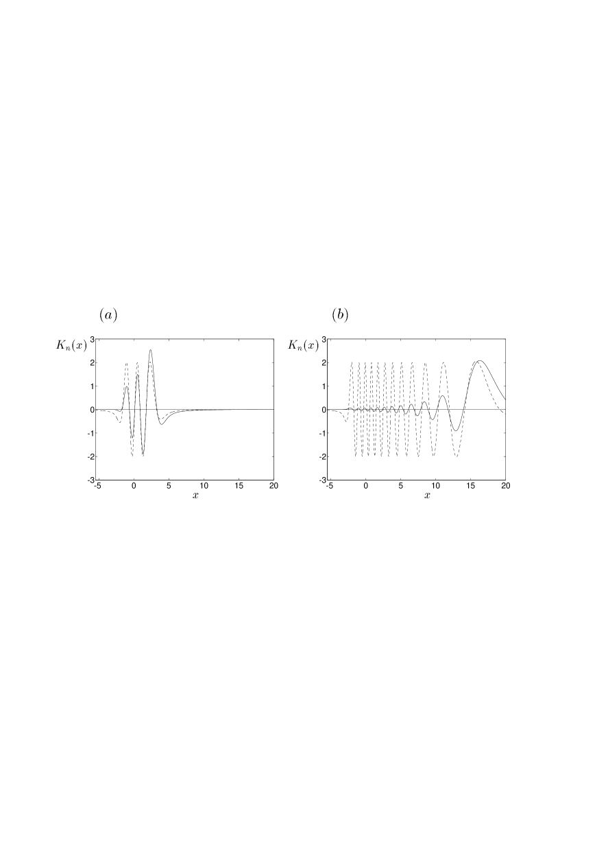
FIG. 1.: Sampling functions for reconstructing the diagonal density-matrix elements $\varrho_{n,n}$ of a Morse oscillator ($a$ $\!=$ $\!0.279$) from the position distribution for $n$ $\!=$ $\!2$ (a) and $n=11$ (b); full line: least-squares method; dashed line: IWM.

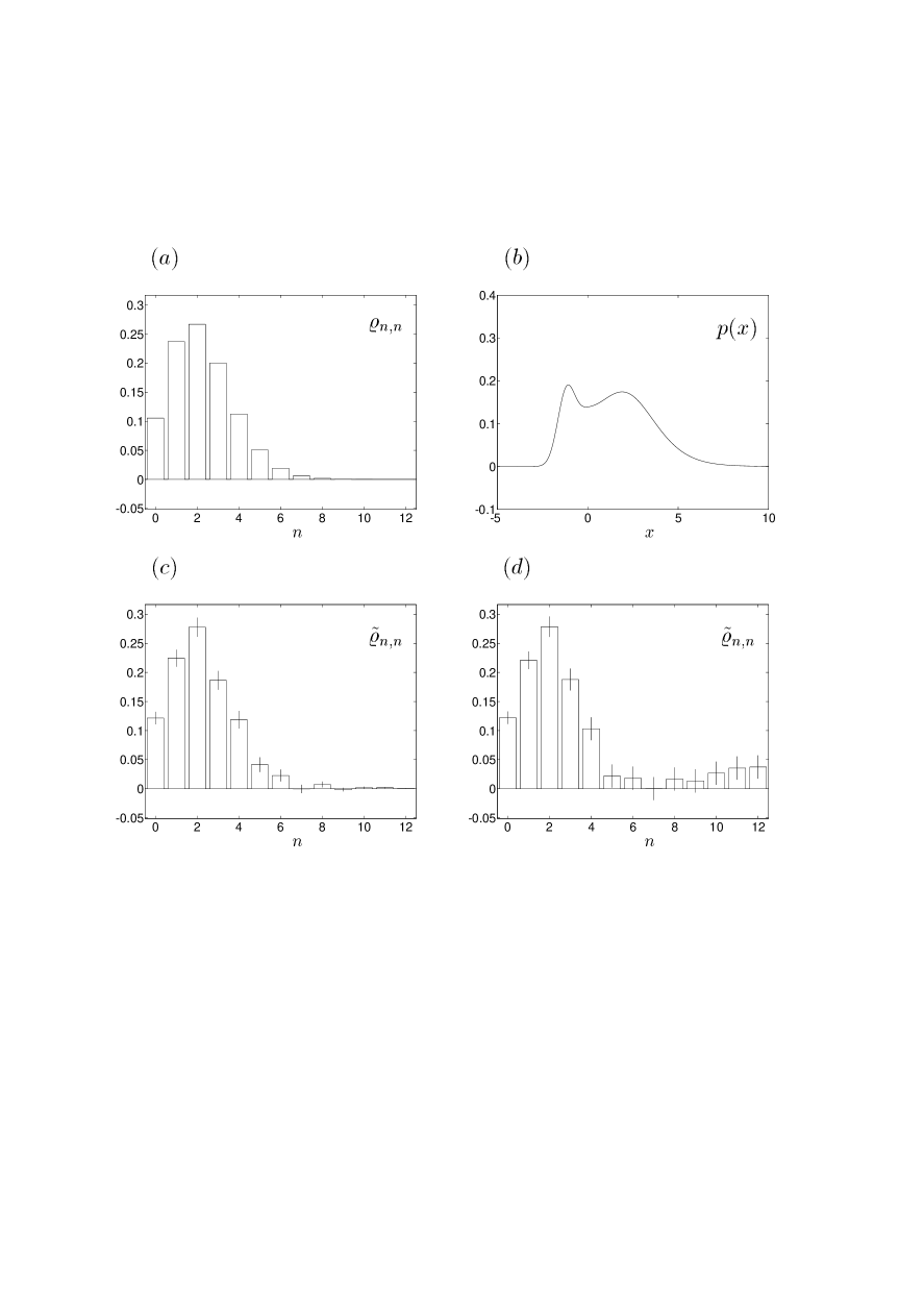
FIG. 2.: Reconstruction of the diagonal density-matrix elements of a Morse oscillator ($a$ $\!=$ $\!0.279$), which is assumed to be prepared in a state $\langle n|\psi\rangle$ $\!\propto$ $\!\alpha^{n}n!^{-1/2}$, $\alpha$ $\!=$ $\!-1.5$, from $N_{\rm e}$ $\!=$ $\!5\times 10^{3}$ recorded events in a simulated position measurement; exact density-matrix elements $\varrho_{n,n}$ (a), exact time-averaged position distribution (b), density-matrix elements $\tilde{\varrho}_{n,n}$ reconstructed using least-squares inversion (c) and IWM (d). The error bars indicate the predicted statistical error (half error bar corresponds to a single standard deviation).

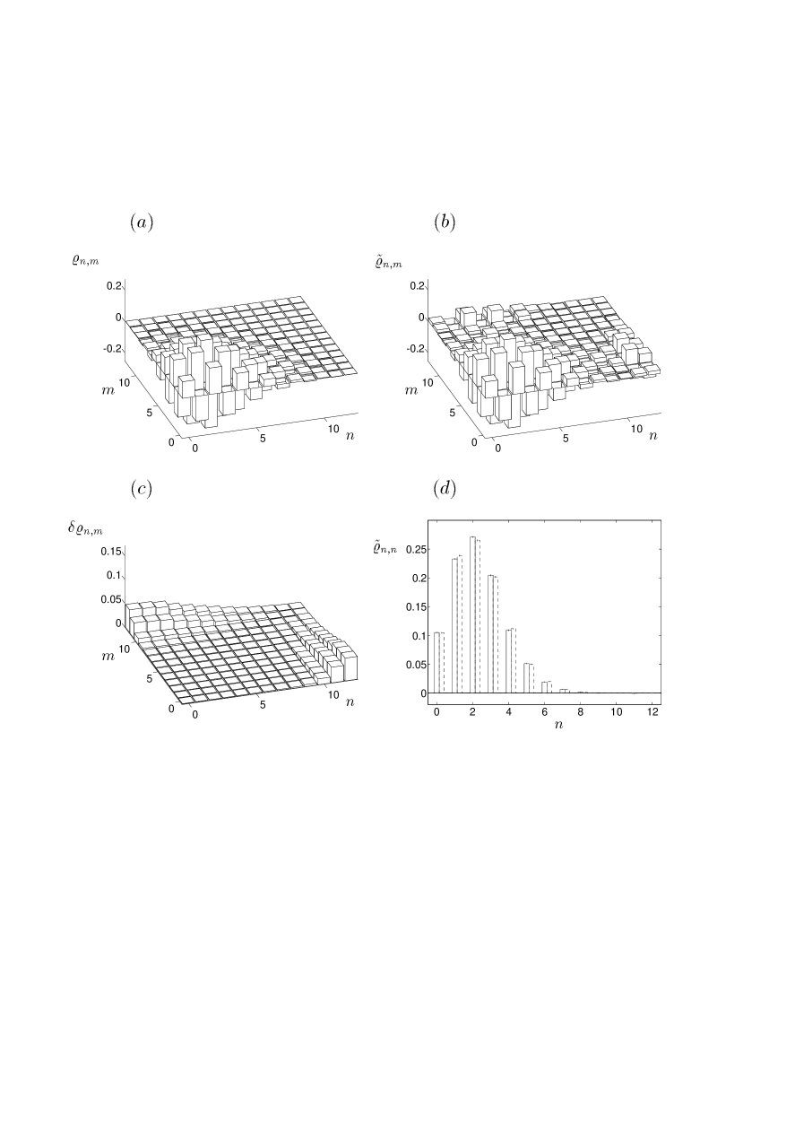
FIG. 3.: Reconstruction of the density-matrix elements of the same system as in Fig. 2 from the data of a simulated position measurement, in which at each of $N_{\rm t}$ $\!=$ $\!120$ equidistant times $N_{\rm e}$ $\!=$ $\!5\times 10^{3}$ events are recorded, the overall time interval being $T$ $\!=$ $\!6\pi/(\omega_{1}-\omega_{0})$; exact density-matrix elements $\varrho_{n,m}$ (a), reconstructed (real parts of the) density-matrix elements $\tilde{\varrho}_{n,m}$ (b), predicted statistical error $\delta\varrho_{n,m}$ (c), comparison of the diagonal elements obtained from the data recorded during the actual measurement time $T$ (full lines) with the diagonal elements obtained (for the same total number of events) in the case when $T$ $\!\to$ $\!\infty$ (dashed lines) (d).

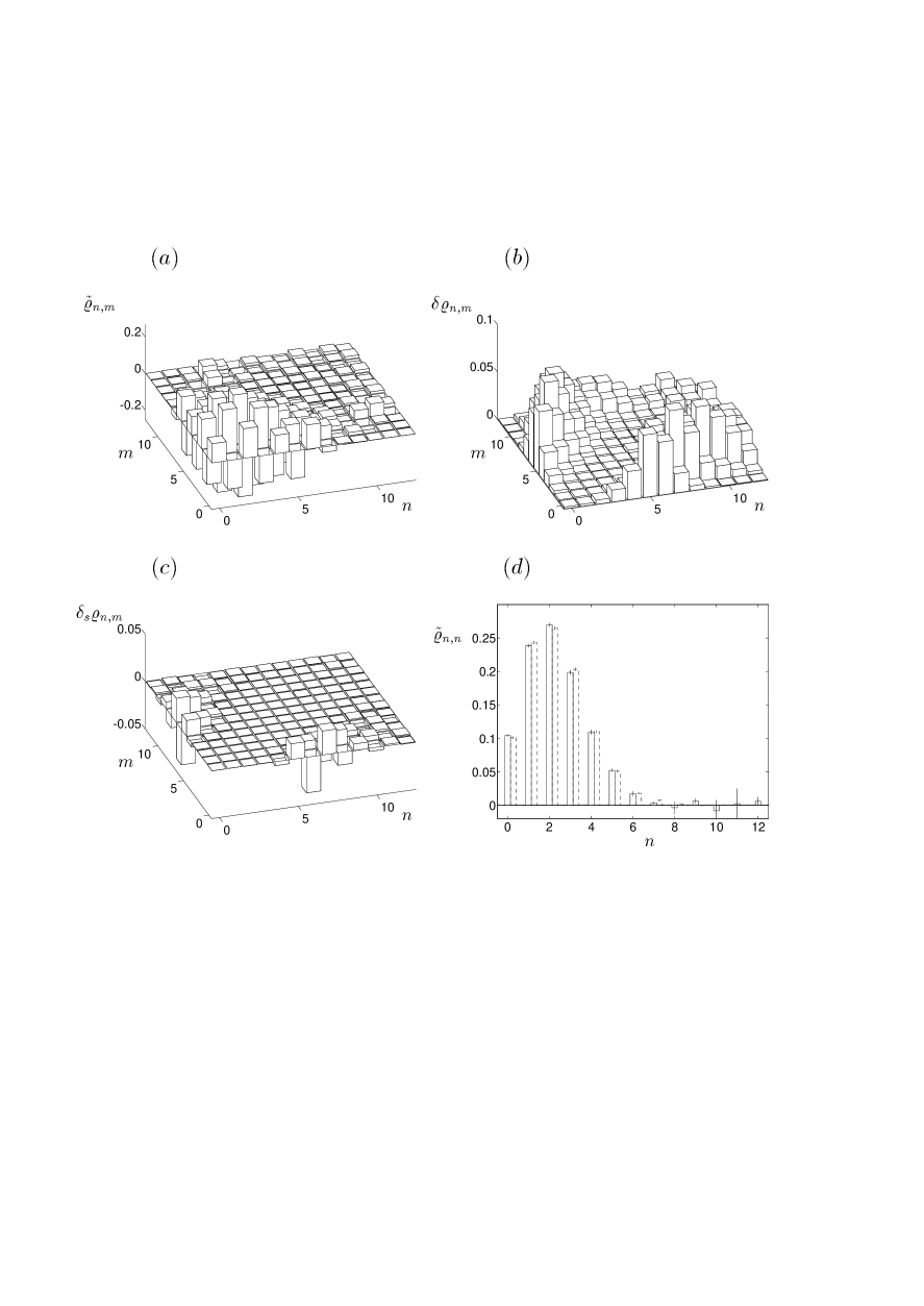
FIG. 4.: Reconstruction of the density-matrix elements of the same system as in Fig. 2 from a simulated measurement of the smeared distribution $\bar{p}(x,t)$ [$\sigma_{t}$ $\!=0.2$ $\!\pi/(\omega_{1}-\omega_{0})$, $\sigma_{x}$ $\!=$ $\!0.3$] at $N_{\rm t}$ $\!=$ $\!30$ equidistant times [during the observational time $T$ $\!=$ $\!6\pi/(\omega_{1}-\omega_{0})$] and $N_{\rm x}$ $\!=$ $\!15$ equidistant positions [in the interval $-2$ $\!\leq$ $\!x$ $\!\leq$ $\!10$] for a total number of events of $N_{\rm tot}$ $\!=$ $\!10^{5}$, using Tikhonov regularization with $\lambda$ $\!=$ $\!2\times 10^{-3}$; reconstructed (real parts of the) density-matrix elements $\tilde{\varrho}_{n,m}$ (a), predicted statistical error $\delta\varrho_{n,m}$ (b), systematical error $\delta_{\rm s}\varrho_{n,m}$ due to regularization (c), comparison of the diagonal elements obtained from the smeared data recorded during the actual measurement time $T$ (full lines) with the diagonal elements obtained (for the same total number of events) without data smearing, and $T$ $\!\to$ $\!\infty$ (dashed lines) (d).

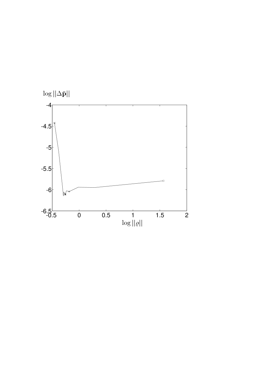
FIG. 5.: The $L$ curve for the problem considered in Fig. 4; $\lambda=10^{-4}$ ($o$), $2\times 10^{-3}$ ($+$), $5\times 10^{-3}$ ($*$), $5\times 10^{-2}$ ($\times$).

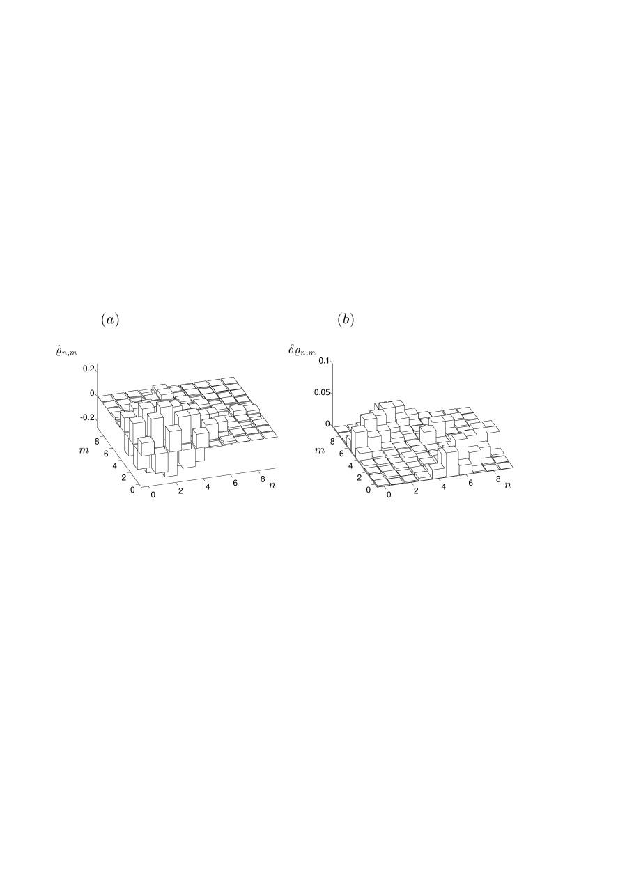
FIG. 6.: Reconstruction of the density-matrix elements of a system of the type considered in Fig. 2, but with smaller anharmonicity, $a$ $\!=$ $\!0.15$, and a truncation parameter smaller than the number of bound states, $n_{\rm max}$ $\!=$ $\!9$, from a simulated measurement of the smeared distribution $\bar{p}(x,t)$ [$\sigma_{t}$ $\!=0.2$ $\!\pi/(\omega_{1}-\omega_{0})$, $\sigma_{x}$ $\!=$ $\!0.3$] at $N_{\rm t}$ $\!=$ $\!30$ equidistant times [during the observational time $T$ $\!=$ $\!4\pi/(\omega_{1}-\omega_{0})$] and $N_{\rm x}$ $\!=$ $\!15$ equidistant positions [in the interval $-2$ $\!\leq$ $\!x$ $\!\leq$ $\!10$] for a total number of events of $N_{\rm tot}$ $\!=$ $\!10^{6}$, using Tikhonov regularization with $\lambda$ $\!=$ $\!10^{-3}$; reconstructed (real parts of the) density-matrix elements $\tilde{\varrho}_{n,m}$ (a), predicted statistical error $\delta\varrho_{n,m}$ (b).

REFERENCES

- [1] Permanent address: Palacký University, Faculty of Natural Sciences, Svobody 26, 77146 Olomouc, Czech Republic.
- [2] K. Vogel and H. Risken, Phys. Rev. A40, 2847 (1989).
- [3] D.T. Smithey, M. Beck, M.G. Raymer, and A. Faridani, Phys. Rev. Lett. 70, 1244 (1993); D.T. Smithey, M. Beck, J. Cooper, M. G. Raymer, and A. Faridani, Phys. Scr. T48, 35 (1993).
- [4] H. Kühn, D.-G. Welsch, and W. Vogel, J. Mod. Opt. 41, 1607 (1994); W. Vogel and D.-G. Welsch, Lectures on Quantum Optics (Akademie-Verlag, Berlin, 1994); A. Zucchetti, W. Vogel, M. Tasche, and D.-G. Welsch, Phys. Rev. A 54, 1678 (1996).
- [5] G.M. D’Ariano, C. Macchiavello, and M.G.A. Paris, Phys. Rev. A 50, 4298, (1994); G.M. D’Ariano, Quantum Semiclass. Opt. 7, 693 (1995); G.M. D’Ariano, U. Leonhardt, and H. Paul, Phys. Rev. A52, R1881 (1995); U. Leonhardt, H. Paul, and G.M. D’Ariano, Phys. Rev. A52, 4899 (1995); H. Paul, U. Leonhardt, and G.M. D’Ariano, Acta Phys. Slov. 45, 261 (1995); U. Leonhardt, M. Munroe, T. Kiss, Th. Richter and M.G. Raymer, Opt. Commun. 127, 144 (1996).
- [6] S. Schiller, G. Breitenbach, S.F. Pereira, T. Müller, and J. Mlynek, Phys. Rev. Lett. 77, 2933 (1996).
- [7] T.J. Dunn, I.A. Walmsley, and S. Mukamel, Phys. Rev. Lett. 74, 884 (1995).
- [8] M.G. Raymer, M. Beck, and D.F. McAlister, Phys. Rev. Lett. 72, 1137 (1994); U. Janicke and M. Wilkens, J. Mod. Opt. 42, 2183 (1995); C. Kurtsiefer, T. Pfau, and J. Mlynek, unpublished.
- [9] S. Wallentowitz and W. Vogel, Phys. Rev. Lett. 75, 2932 (1995), Phys. Rev. A 54, 3322 (1996); J.F. Poyatos, R. Walser, J.I. Cirac, and P. Zoller, Phys. Rev. A 53, R1966 (1996); C. D’Helon and G.J. Milburn, Phys. Rev. A 54, R25 (1996).
- [10] N.G. Walker and J.E. Caroll, Electron. Lett. 20, 981 (1984); M. Freyberger, K. Vogel, and W.P. Schleich, Phys. Lett. 176A, 41 (1993); G.S. Agarwal and S. Chaturvedi, Phys. Rev. A42, R665 (1994); A. Zucchetti, W. Vogel, and D.-G. Welsch, Phys. Rev. A54, 856 (1996).
- [11] S. Wallentowitz and W. Vogel, Phys. Rev. A 53, 4528 (1996); K. Banaszek and K. Wódkiewicz, Phys. Rev. Lett. 76, 4344 (1996).
- [12] T. Opatrný and D.-G. Welsch, Phys. Rev. A 55, 1462 (1997); T. Opatrný, D.-G. Welsch, S. Wallentowitz, and W. Vogel, Quantum State Reconstruction by Multichannel Unbalanced Homodyning, submitted to J. Mod. Optics.
- [13] D. Leibfried, D.M. Meekhof, B.E. King, C. Monroe, W.M. Itano, and D.J. Wineland, Phys. Rev. Lett. 77, 4281 (1996).
- [14] T.J. Dunn, J.N. Sweetser, I.A. Walmsley, and C. Radzewicz, Phys. Rev. Lett. 70, 3388 (1993).
- [15] M.W. Noel and C.R. Stroud, Jr., Phys. Rev. Lett. 77, 1913 (1996).
- [16] M. Shapiro, J. Chem. Phys. 103, 1748 (1995).
- [17] U. Leonhardt and M.G. Raymer, Phys. Rev. Lett. 76, 1989 (1996); U. Leonhardt, Acta Phys. Slovaca 46, 309 (1996); Th. Richter and A. Wünsche, Phys. Rev. A 53, R1974 (1996); Th. Richter, Phys. Lett. A 211, 327 (1996); Th. Richter and A. Wünsche, Acta Phys. Slovaca 46, 487 (1996).
- [18] P. Kowalczyk, C. Radzewicz, J. Mostowski, and I.A. Walmsley, Phys. Rev. A 42, 5622 (1990); L. Waxer, I.A. Walmsley, and W. Vogel, Phys. Rev. A, to be published.
- [19] A.M. Legendre, Nouvelles méthodes pour la détermination des orbites des comètes (Firmin - Didot, Paris, 1805); C.F. Gauss, Theoria motus corporum coelestium in sectionibus conicis solem ambientum (Perthes and Besser, Hamburg, 1809); Theoria combinationis observationum erroribus minimis obnoxiae (Societati regiae scientiarum exhibita, Göttingen, 1821).
- [20] P.J. Bardroff, E. Mayr, W.P. Schleich, P. Domokos, M. Brune, J.M. Raimond, and S. Haroche, Phys. Rev. A 53, 2736 (1996).
- [21] S.M. Tan, An Inverse Problem Approach to Optical Homodyne Tomography, submitted to J. Mod. Optics.
- [22] U. Leonhardt, Phys. Rev. A, to be published.
- [23] P.M. Morse, Phys. Rev. 34, 57 (1929).
- [24] G.M. D’Ariano, C. Macchiavello, and M.G.A. Paris, Optics Commun. 129, 6 (1996).
- [25] T. Kiss, U. Herzog, and U. Leonhardt, Phys. Rev. A 52, 2433 (1995); U. Herzog, Phys. Rev. A 53, 1245 (1996).
- [26] V. Bužek, G. Adam, and G. Drobný, Ann. Phys. (NY) 245, 37 (1996).
- [27] H. Wiedemann, Quantum Tomography with the Maximum Entropy Principle, submitted to Phys. Rev. A.
- [28] Z. Hradil, Phys. Rev. A, to be published.
- [29] D.J.S. Robinson, A Course in Linear Algebra with Applications (World Scientific, Singapore, 1991). G.H. Golub and C.F. van Loan, Matrix Computations (J. Hopkins University Press, Baltimore and London, 1989); W.H. Press, S.A. Teukolsky, W.T. Vetterling, and B.P. Flannery, Numerical Recipes in C (Cambridge University Press, New York, 1995).