Research Institute for Theoretical Physics University of Helsinki
Preprint series in Theoretical Physics, HU-TFT-96-43, 25 November 1996

We consider the time evolution of a discrete state embedded in a continuum. Results from scattering theory can be utilized to solve the initial value problem and discuss the system as a model of wave packet preparation. Extensive use is made of the analytic properties of the propagators, and simple model systems are evaluated to illustrate the argument. We verify the exponential appearence of the continuum state and its propagation as a localized wave packet.

This article will appear in a Special Issue of Journal of Modern Optics in 1997

1 Introduction

Quantum mechanics knows many examples of discrete states coupled to a continuum. Much work has been devoted to these problems in the past. In this paper we are going to review these works briefly, but reconsider them as methods to prepare time dependent states. All tunnelling problems are of this type, but in addition we have similar phenomena occurring when a photon excitation is followed by leakage into continuous outgoing states.

A simple physical example is provided by autoionization, where an excited state is coupled to atomic ionization according to

$$A+\hbar\omega\rightarrow A^{*}\rightarrow A^{+}+e^{-}.$$ (1.1)

In molecules, the analogous process is the predissociation reaction

$$AB+\hbar\omega\rightarrow AB^{*}\rightarrow A+B,$$ (1.2)

and in chemical reactions the transition state may give a similar behaviour

$$AB+C+\hbar\omega\rightarrow ABC^{*}\rightarrow A+BC.$$ (1.3)

In a nucleus, $ABC^{*}$ would be a compound nucleus or a doorway state. In particle physics, the particle production processes provide additional examples.

When the final states form a continuous spectrum, the decay of the initially prepared state is often described by an exponential. This was first derived from quantum theory by Landau [1], but the procedure is usually referred to by the names Weisskopf and Wigner [2]. These features were found to appear exactly in the treatment of the Lee model [3], where, however, the primary interest was devoted to the renormalizability of the theory. The appearance of decay as a consequence of the analytic properties of the propagators became a central issue for the theoretical discussion after Peierls had pointed out that the functions needed to be continued to the second Riemann sheet [4]. These discussions can be found in Refs. [5] and [6], and the results are summarized in the context of scattering theory in the text book [7].

When several singularities are close to each other or multiple poles occur, there appears non-exponential time dependence as discussed by Mower [8]; the corresponding problem for a generalized Lee-model is treated in Ref. [9]. In molecules the high density of states gives rise to a similar physical situation through nonradiative transfer of excitation; for a review of this theory see Ref. [10]. Many more works from this early period could be cited, but these may suffice for the present.

The works above are mainly formulated as scattering problems and, except for the evaluation of probability decay, they tend not to look into the detailed time evolution of the processes. The use of well controlled laser pulses in the femtosecond time range has recently made it possible to follow microscopic processes in space and time [11]. Thus one may resolve the Schrödinger propagation following a fast preparation of an initial state. It is then interesting to reconsider the theories above from the point of view of state preparation. If we excite a resolved initial state coupled to a continuum, which kind of wave packet can we prepare into the continuum? How is this state emerging and how is it propagating?

This can be seen as a continuation of our earlier work on molecular dynamics [12] and on electrons in semiconductor structures [13]. Here we consider explicitly the time dependence following an initial preparation. Our state functions can thus stay normalized at all times in contrast to the situation in a scattering description. Thus we can avoid paradoxes of exponentially growing amplitudes such as discussed by Peierls in Ref. [14].

The preparation of well localized wave packets is an interesting and challenging problem in atomic physics. Various excitation processes have produced electronic wave packets on bound Rydberg manifolds; see e.g. Refs. [15] and [16], but it is not clear if these can be launched into freely propagating states. Molecular dissociation, following coherent excitation from the ground state [12], is expected to prepare localized wave packets in the reaction coordinate. In simple cases, this can be seen as propagation in the laboratory too. To prepare electronic wave packets in semiconductors poses huge experimental difficulties [17]; to retain their coherence seems almost impossible. Excitonic wave packets dephase more slowly, but their theoretical description is even more difficult.

In this paper we adopt the presumption that an experimental procedure exists to prepare a pure isolated state. The interaction with the continuum is set in, and we can follow both the growth of the continuum states and the decay of the initial one. This makes it possible to consider the process as a state preparation. We can describe the disappearance of the initial state and the growth and propagation of the state prepared in the continuum.

In order to achieve our goal, we postulate the validity of a simple model Hamiltonian. It is of the Lee model type and can hence be solved exactly to give formal expressions for all quantities of interest. In order to treat the initial value problem we utilize the Laplace transform, but in order to retain agreement with the conventional Fourier transform treatments, we denote the Laplace transform variable by $-i\omega$; the resulting transform is named the Laplace-Fourier transform (${\cal LF}$-transform).

We present the model in Sec. 2 and its formal solution in Sec. 3, where also the general behaviour of the solution is discussed. In Sec. 4 we present some simple models which illustrate the features of the general discussion.

In Sec. 4.1 we assume that the continuum spectral density can be described by a simple complex pole, the generalization to several poles is straightforward. This approximation has acquired renewed interest after Garraway [18] has showed that the multiple pole approximation can be put into a Lindblad form amenable to a Monte Carlo simulation in terms of hypothetical pseudomodes, which describe the non-Markovian effects. However, he finds that consistency may require that the pseudomodes are coupled in their Hamiltonian.

Section 4.2 presents a simple model where the role of analytic continuation can be elucidated and the exact behaviour of the wave packet in the continuum can be calculated. The role of the process as a preparation is clearly seen in this model. In Sec. 4.3 we try to construct a physical system having the properties of our earlier models. This is selected from the field of molecular physics [12] and tests how weak coupling to a molecular continuum can be utilized to prepare a wave packet. We find that this is, indeed, possible, but the system has got many complementary features which we will discuss in a forthcoming paper.

Section 5 presents a brief discussion of our results and the conclusions.

2 The model calculation

We are considering a model with one single state embedded in a continuum. This is described by the Hamiltonian

$$\begin{array}[]{lll}H&=&H_{0}+V\\ &&\\ H_{0}&=&\omega_{0}\mid 0\rangle\langle 0\mid+\int d\epsilon\mid\epsilon\rangle\,\epsilon\,\langle\epsilon\mid\\ &&\\ V&=&\int d\epsilon\;\left(V_{\epsilon}\mid\epsilon\rangle\langle 0\mid+V_{\epsilon}^{*}\mid 0\rangle\langle\epsilon\mid\right)\end{array}$$ (2.1)

in an obvious notation. Observe that this is the form of a general tunnelling Hamiltonian. The initial state is supposed to be the isolated state

$$\mid\psi(t=0)\rangle=\mid 0\rangle.$$ (2.2)

Because we are going to consider time evolution, we introduce the Laplace-Fourier transform in the form

$$\widetilde{\psi}(\omega)=-i\int\limits_{0}^{\infty}dt\,e^{i\omega t}\psi(t)\,\equiv{\cal LF}(\psi).$$ (2.3)

This gives us analytic functions in the conventional half-plane ${\rm Im}(\omega)\geq 0$. We have the usual properties

$$\begin{array}[]{lll}{\cal LF}(\dot{\psi})&=&-i\left(\omega\widetilde{\psi}(\omega)-\psi(t=0)\right)\\ &&\\ \lim\limits_{\omega\rightarrow\infty}\left(\omega\widetilde{\psi}(\omega)\right)&=&\psi(t=0)\equiv\psi_{0}\\ &&\\ \lim\limits_{\omega\rightarrow 0}\left(\omega\widetilde{\psi}(\omega)\right)&=&\psi(t=\infty).\end{array}$$ (2.4)

The inversion is achieved by

$$\psi(t)=\frac{i}{2\pi}\int\limits_{-\infty+ia}^{+\infty+ia}e^{-i\omega t}\;\widetilde{\psi}(\omega)\,dt,$$ (2.5)

where $a>0$. With these definitions the solution of the Schrödinger equations is given by

$$\widetilde{\psi}(\omega)=G(\omega)\psi_{0},$$ (2.6)

where the propagator is

$$G(\omega)=\frac{1}{\omega-H}.$$ (2.7)

It is easy to verify the consistency of these relations.

We are now going to partition the problem above in order to separate the time evolution of the single state and that of the continuum. Thus we introduce the projectors

$$\begin{array}[]{lll}P&=&\mid 0\rangle\langle 0\mid\\ &&\\ Q&=&1-P=\int d\epsilon\mid\epsilon\rangle\,\langle\epsilon\mid.\end{array}$$ (2.8)

Both projectors commute with the Hamiltonian $H_{0}.$

The results that we need were derived long ago in scattering theory, but for easy reference we summarize them in the Appendix. We introduce the definition

$$O^{XY}\equiv XOY,$$ (2.9)

where $O$ is any operator and $X,Y=P$ or $Q;$ the operators $O^{XX}$ are denoted by $O^{X}$ simply.

We introduce a connected operator $\Gamma$ which has the single state pole removed from the intermediate states by writing

$$\Gamma=V+V\,G_{0}^{Q}\,\Gamma,$$ (2.10)

where the unperturbed propagator is

$$G_{0}(\omega)=\frac{1}{\omega-H_{0}}.$$ (2.11)

In terms of this operator, we can now write the exact solution for all the propagators needed in the form

$$G^{P} = \left((G_{0}^{P})^{-1}-\Gamma^{P}\right)^{-1}$$ (2.12)

$$G^{QP} = G_{0}^{Q}V^{QP}G^{P}$$ (2.13)

$$G^{Q} = G_{0}^{Q}+G_{0}^{Q}\left(\Gamma^{Q}+\Gamma^{QP}G^{P}\Gamma^{PQ}\right)G_{0}^{Q}.$$ (2.14)

Thus we can obtain all desired partitioned propagators if we can solve the integral equation (2.10). In the present case, this can be solved trivially if we notice that

$$V^{P}=V^{Q}=0.$$ (2.15)

From this it follows that

$$\begin{array}[]{lll}\Gamma^{QP}&=&V^{QP}\\ &&\\ \Gamma^{P}&=&V^{PQ}G_{0}^{Q}V^{QP}.\end{array}$$ (2.19)

This gives the solutions

$$\langle 0\mid G\mid 0\rangle = \frac{1}{\omega-\omega_{0}-\Sigma(\omega)}$$ (2.20)

$$\langle\epsilon\mid G\mid 0\rangle = \left(\frac{1}{\omega-\epsilon}\right)V_{\epsilon}\left(\frac{1}{\omega-\omega_{0}-\Sigma(\omega)}\right)$$ (2.21)

$$\langle\epsilon\mid G\mid\epsilon^{{}^{\prime}}\rangle = \frac{\delta(\epsilon-\epsilon^{{}^{\prime}})}{\omega-\epsilon}+\left(\frac{V_{\epsilon}\,}{\omega-\epsilon}\right)\left(\frac{V_{\epsilon^{\prime}}^{*}}{\omega-\epsilon^{{}^{\prime}}}\right)\left(\frac{1}{\omega-\omega_{0}-\Sigma(\omega)}\right).$$ (2.22)

The self-energy function is given by

$$\Sigma(\omega)=\langle 0\mid\Gamma\mid 0\rangle=\int d\epsilon\left(\frac{D(\epsilon)}{\omega-\epsilon}\right),$$ (2.23)

where we have introduced the spectral density

$$D(\epsilon)=\mid V_{\epsilon}\mid^{2}\geq 0.$$ (2.24)

This notation is preferable because we can then include a density-of-states function in the spectral density $D(\omega)$ when needed.

With the initial condition (2.2) we find the amplitude of the isolated state to be

$$A(t)\equiv\langle 0\mid e^{-iHt}\mid 0\rangle=\frac{i}{2\pi}\int\limits_{-\infty+ia}^{+\infty+ia}e^{-i\omega t}\;\left(\frac{1}{\omega-\omega_{0}-\Sigma(\omega)}\right)\,dt.$$ (2.25)

Because the integrated function is analytic in the upper half plane, the time evolution is determined by the singularities of the integrand on the real axis and below. We are thus looking for solutions of the equation

$$h(\omega)\equiv\omega-\omega_{0}-\Sigma(\omega)=0.$$ (2.26)

As can be seen from Eq. (2.23) the function $\Sigma(\omega)$ has got a branch cut along the real axis. Its weight is given by $D(\omega).$

3 General properties of the solution

From the definition (2.23) it follows directly that

$${\rm Im}\,\Sigma(\omega\pm i\eta)=\mp\pi D(\omega);$$ (3.1)

it is assumed that $\eta\rightarrow 0.$ Consequently, the function has a branch cut at every value of $\omega$ such that $D(\omega)$ differs from zero.

All physical systems have energies bounded from below, thus all integrals over the variable $\epsilon$ must start at a finite value $\mu.$ If the energy of the isolated state lies below this spectral cut-off

$$\omega_{0}<\mu,$$ (3.2)

the continuum only serves to renormalize the state. Then we may write

$$\Sigma(\omega)=\int d\epsilon\;\frac{D(\epsilon)}{\omega-\omega_{0}-(\epsilon-\omega_{0})}=\int d\epsilon\;\frac{D(\epsilon)}{(\omega_{0}-\epsilon)}-\int d\epsilon\;\frac{D(\epsilon)}{(\omega_{0}-\epsilon)^{2}}\;\left(\omega-\omega_{0}\right)+...$$ (3.3)

This gives the propagator (2.20) the form

$$\langle 0\mid G\mid 0\rangle=\frac{Z}{\omega-\tilde{\omega}_{0}},$$ (3.4)

where the state renormalization constant is given by

$$Z=\left(1+\int d\epsilon\;\frac{D(\epsilon)}{(\omega_{0}-\epsilon)^{2}}\right)^{-1}$$ (3.5)

and the renormalized energy is

$$\tilde{\omega}_{0}=\omega_{0}+Z\int d\epsilon\;\frac{D(\epsilon)}{(\omega_{0}-\epsilon)}<\omega_{0}.$$ (3.6)

These results are valid to order $\left(\frac{\omega_{0}-\tilde{\omega}_{0}}{\mu-\omega_{0}}\right)$, and we still have $\tilde{\omega}_{0}<\mu$. The only effect of the continuum is to push the isolated level away and decrease the overlap between the initial bare state and the renormalized state to $Z<1$. This state does not decay but continues oscillating with the frequency $\tilde{\omega}_{0}$ forever. The reminder of the initial state is lost into the continuum as the coupling is switched on.

When the isolated state is embedded in the continuum, $\omega_{0}>\mu$, it can decay. In the equation (2.25) we require the zeros of the function $h(\omega)$ to be in the lower half plane. Let us see if such singularities exist by setting

$$\omega=\omega^{\prime}-i\omega^{\prime\prime}$$ (3.7)

into $h(\omega)$. We find

$$\omega^{\prime}-i\omega^{\prime\prime}-\omega_{0}-\int d\epsilon\;\frac{D(\epsilon)}{\omega^{\prime}-i\omega^{\prime\prime}-\epsilon}=0.$$ (3.8)

Separating the real and imaginary parts of this equation should fix the oscillational frequency $\omega^{\prime}$ and the damping $\omega^{\prime\prime}.$ We write down the imaginary part as

$$\omega^{\prime\prime}\left(1+\int d\epsilon\;\frac{D(\epsilon)}{\left(\omega^{\prime}-\epsilon\right)^{2}+\left(\omega^{\prime\prime}\right)^{2}}\right)=0.$$ (3.9)

This equation obviously lacks solutions $\omega^{\prime\prime}\neq 0$ and does not correspond to a physical result. This is obtained when we remember that the physical values of $\omega$ approach the real axis from the upper half plane, and we should thus look for zeros when the function $\Sigma(\omega)$ is continued analytically into the lower half plane. This procedure will provide the singularities giving a contribution to the integral (2.25). We consequently need to continue $\Sigma(\omega)$ across the real axis as discussed by Peierls [18].

The simplest manner to do this is to push the integration contour in Eq. (2.25) down below the real axis. Any isolated pole encountered in this manner is included as a single contribution to the time evolution in the manner shown in Fig. 1. For one single pole this works well, and the result is simple exponential decay as in the Weisskopf-Wigner approach. However, with several singularities only well isolated poles can be treated this way. When the poles are close to each other, this method cannot be justified, because its validity is based on a series expansion like that in Eq. (3.3) around each singularity; the radius of convergence can only be extended to the nearest singularity, and hence close lying poles interfere [8]. Another limitation comes from the lower cut-off in the spectral weight $D(\omega)$. Because $D(\omega)=0$ for $\omega<\mu$, this end point must be a singularity of the function. Thus there is a branch cut starting here, which can be moved around but must be pinned down at $\omega=\mu$. Poles too close to this cut-off cannot have a large radius of convergence and hence the branch cut cannot be neglected in their treatment. In particle theory these cuts derive from particle creation thresholds.

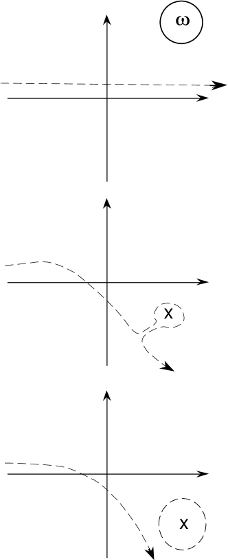
Figure 1: In the complex $\omega$-plane, the Laplace-Fourier transform is inverted by integration along the line $[-\infty+ia,+\infty+ia].$ The analytic continuation can be effected by moving the contour into the lower half-plane. When a pole is encountered, the contour must circle it, but can continue down leaving the pole encircled by an isolated contour.

In the region where $D(\omega)$ is an analytic function of $\omega$, we can achieve the analytic continuation of the self-energy by defining the new function

$$\Sigma^{+}(\omega)=\int d\epsilon\left(\frac{D(\epsilon)}{\omega-\epsilon}\right)-2\pi iD(\omega).$$ (3.10)

Using (3.1) one can easily verify that the function $\Sigma^{+}(\omega)$ has no singularity when the real axis is crossed from above. When this process works, it is a simple way to look for singularities on the second sheet of the lower half plane.

When the result (3.10) is inserted into the equation (2.26) we find the relation

$$\omega^{{}^{\prime}}-\omega_{0}-\int d\epsilon\,D(\epsilon)\left(\frac{\omega^{{}^{\prime}}-\epsilon}{\left(\omega^{{}^{\prime}}-\epsilon\right)^{2}+\omega^{{}^{\prime\prime}2}}\right)+2\pi\frac{\partial D(\omega^{{}^{\prime}})}{\partial\omega}\omega^{{}^{\prime\prime}}=0,$$ (3.11)

where we have anticipated that the imaginary part is small. In addition we have

$$\omega^{{}^{\prime\prime}}=2\pi iD(\omega^{{}^{\prime}})-\int d\epsilon\,D(\epsilon)\left(\frac{\omega^{{}^{\prime\prime}}}{\left(\omega^{{}^{\prime}}-\epsilon\right)^{2}+\omega^{{}^{\prime\prime}2}}\right).$$ (3.12)

The values of the oscillational frequency $\omega^{{}^{\prime}}$ and the damping $\omega^{{}^{\prime\prime}}$ are determined by the coupled equations (3.11) and (3.12). The oscillational part determined from (3.11) is discussed in detail by Cohen-Tannoudji [20]. In the limit $\omega^{{}^{\prime\prime}}\rightarrow 0$ the results simplify. When the damping is small, we obtain

$$\omega^{{}^{\prime\prime}}\Rightarrow\pi D(\omega),$$ (3.13)

which directly provides a consistency check. The Weisskopf-Wigner result thus emerges in the weak coupling limit from our prescription for analytic continuation.

It is instructive to realize that in the weak coupling limit, the prescription we have used for analytic continuation is to replace $\Sigma(\omega)$ just below the real axis by its value just above; i.e. we are performing an analytic continuation using only the zeroth order term in a Taylor expansion across the real axis. Thus the analytically continued equation (3.8) becomes

$$\omega^{\prime}-i\omega^{\prime\prime}-\omega_{0}-\int d\epsilon\;\frac{D(\epsilon)}{\omega^{\prime}+i\omega^{\prime\prime}-\epsilon}=0.$$ (3.14)

For small values of $\omega^{\prime\prime}$ this gives back all results derived previously. It is to be noted that, inside the integral, the precise value of $\omega^{\prime\prime}$ does not affect the result, and we can obtain the correct damping using the conventional infinitesimal $i\eta$ prescription. Our discussion is in fact a derivation of this rule.

An instructive way to consider the equation (3.14) is to regard the imaginary part in the denominator as a small dissipative part of the energies in the continuum

$$\epsilon-i\omega^{\prime\prime}\Rightarrow\epsilon-i\epsilon^{{}^{\prime}}.$$ (3.15)

This provides an interesting physical interpretation of the results. Adding any minute dissipative mechanism to the continuum we will find that the isolated state will decay with the rate (3.13) independently of the details of the dissipation of the continuum. Thus any system coupled perturbatively to a dissipative probability sink through a continuum will decay with a rate determined by the coupling strength and not by the actual dissipation of the continuum. In the perturbative limit, the probability flow into the continuum will be the bottleneck. The dissipated continuum acts as a proper reservoir unable to return the probability once it has received it. This interpretation of the procedure directly provides the right sign in the denominator of (3.14) to effect the proper analytic continuation.

When we calculate the integral in Eq. (2.25), we distort the contour into the lower half plane until we encounter the pole defined by (3.11) and separate a contour $c_{0}$ circling this. If no other singularity were encountered, we could pull the contour to negative imaginary infinity and find no corrections. In a physical system this is, however, impossible because the spectral density $D(\omega)$ has necessarily got the lower limit $\mu$ as explained above. The branch cut starting here is pulled down to $-i\infty$ in the manner shown in Fig. 2. This contributes an additional contour $c_{1}$ as shown in the figure. Thus we find

$$A(t) = \frac{i}{2\pi}\left[\int_{c_{1}}dt\,e^{-i\omega t}\;\left(\frac{1}{\omega-\omega_{0}-\Sigma(\omega)}\right)+\int_{c_{0}}dt\,e^{-i\omega t}\;\left(\frac{1}{\omega-\omega^{{}^{\prime}}+i\omega^{{}^{\prime\prime}}}\right)\right]$$ (3.16)

$$= I_{1}(t)+\exp\left(-i\omega^{{}^{\prime}}t-\omega^{{}^{\prime\prime}}t\right).$$

The second term is as expected in a perturbative calculation of the Weisskopf-Wigner type, and we have taken the residue $Z$ of (3.5) to be unity. The decay rate of the probability is given by the well known expression

$$\gamma=2\omega^{{}^{\prime\prime}}=2\pi D(\omega).$$ (3.17)

However, the corrections from the cut are given as

$$I_{1}(t)=\frac{e^{-i\mu t}}{2\pi}\int\limits_{0}^{\infty}e^{-\xi t}\left(\frac{\Sigma_{I}(\mu-i\xi+\eta)-\Sigma_{II}(\mu-i\xi-\eta)}{\left(\omega-\omega_{0}-\Sigma_{I}\right)\left(\omega-\omega_{0}-\Sigma_{II}\right)}\right)d\xi,$$ (3.18)

where the infinitesimal parameter $\eta$ ensures that the self energy is evaluated on the two sides of the cut. From this form we can see that in the long time limit $t\rightarrow\infty$, only the value $\xi\approx 0$ contributes. This would give no contribution without the singularity of $\Sigma$ across the cut. Thus we can set $\xi=0$ everywhere except in the integral

$$\Sigma_{I}(\mu-i\xi+\eta)-\Sigma_{II}(\mu-i\xi-\eta) = \int_{\mu}^{\infty}d\epsilon\;D(\epsilon)\left[\frac{1}{\mu-i\xi+\eta-\epsilon}-\frac{1}{\mu-i\xi-\eta-\epsilon}\right]$$

$$= \int\limits_{0}^{\infty}d\nu\;D(\mu+i\nu)\left[\frac{1}{\xi+\nu+i\eta}-\frac{1}{\xi+\nu-i\eta}\right]$$

$$= -2\pi iD(\mu+i\xi).$$

Because $\omega=\mu$ is a threshold, we expect that we have

$$D(\mu+i\xi)=\beta\;\left(i\xi\right)^{\alpha}+...$$ (3.20)

for small values of $\xi.$ Inserting this into the equation (3.18), we find the leading term

$$I_{1}(t)=\frac{\beta\,e^{-i\mu t}\;i^{\alpha+3}}{\left(\mu-\omega_{0}-\Sigma(\mu)\right)^{2}}\Gamma(\alpha+1)\left(\frac{1}{t^{\alpha+1}}\right).$$ (3.21)

This type of asymptotic result was given for scattering theory already in Ref. [7]. When the exponential in (3.16) has decayed, the power dependence (3.21) will dominate for long times.

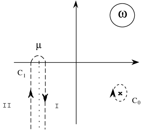
Figure 2: Because physical spectra have a lower limit $\mu$, there must be a branch cut starting at this value. When isolated poles are encircled by closed contours, here $c_{0}$, the branch cut can be drawn from $\mu$ to $-\infty$, thus contributing another contour $c_{1}$.

The treatment given above does, of course, assume that there are no additional poles encountered. If these are well separated, they contribute simply additional exponential terms, but for poles situated close to each other interferences occur; for a discussion of these cf. the discussion by Mower [8].

4 Simple models

4.1 A pole in the spectral density

Many systems display a moderately sharp spectral feature in its density of states. Hence one may often approximate this with a Lorentzian shape, which simplifies the treatment considerably. Such assumptions are often utilized to describe scattering from condensed matter [21], but it is useful in theoretical discussions too. Recently Garraway has utilized it to describe non-Markovian effects in terms of pseudomodes [18].

We assume that the spectral function has the simple shape

$$D(\epsilon)=\frac{A^{2}}{\left(\epsilon-a\right)^{2}+b^{2}}.$$ (4.22)

This satisfies the positivity requirement, but it lacks the lower limit necessary in physical systems. Thus no power law terms are expected.

With the expression (4.22), the analytic continuation to the second sheet is trivial. Inserted into Eqs. (2.23) and (2.20) it gives the results

$$\begin{array}[]{lll}\Sigma(\omega)&=&\frac{\textstyle\pi A^{2}}{\textstyle b}\left(\frac{\textstyle 1}{\textstyle\omega-a+ib}\right)\\ &&\\ \langle 0\mid G(\omega)\mid 0\rangle&=&\frac{\textstyle\omega-a+ib}{\textstyle(\omega-a+ib)(\omega-\omega_{0})-\frac{\textstyle\pi A^{2}}{\textstyle b}}.\end{array}$$ (4.23)

This form is found to satisfy the correct initial condition

$$\lim_{\omega\rightarrow\infty}\omega\langle 0\mid G(\omega)\mid 0\rangle\,\psi(0)=\psi(0).$$ (4.24)

The general solution of the time evolution becomes

$$A(t)=\left(R_{1}\,e^{i\Omega_{+}t}+R_{2}\,e^{i\Omega_{-}t}\right),$$ (4.25)

where $\Omega_{\pm}$ are the two roots of the denominator in Eq. (4.23); from the form of the equation it follows that the sum of the residues is unity: $R_{1}+R_{2}=1$.

Inserting the ansatz (3.7) into the denominator of Eq. (4.23) we find that the imaginary part follows as the solution of the equation

$$\omega^{{}^{\prime\prime}}=\left(\frac{\pi A^{2}}{b}\right)\frac{\left(b-\omega^{{}^{\prime\prime}}\right)}{\left(a-\omega^{{}^{\prime}}\right)^{2}+\left(b-\omega^{{}^{\prime\prime}}\right)^{2}}.$$ (4.26)

Because the right hand side of this equation is positive for $\omega^{{}^{\prime\prime}}<b$ there must be a solution for $0<\omega^{{}^{\prime\prime}}<b$, irrespective of the value of $\omega^{{}^{\prime}}.$ This proves that both roots $\Omega_{\pm}$ have negative imaginary parts and the solution $A(t)$ decays to zero as we expect. Thus the pole approximation is consistent and only fails to reproduce the long time behaviour deriving from the threshold in the spectral density. In a similar manner the appearance of several poles can be discussed. Of special interest is the case when a pole with negative weight is encountered. This case is discussed in detail by Garraway [19].

4.2 The branch cut model

In order to illustrate the concepts introduced in Sec. 3 we introduce a model where the Weisskopf-Wigner result emerges as an exact consequence. It is then possible to follow how the analytic continuation to the physical sheet works in detail, and the correction terms can be evaluated explicitly.

The model is based on the following spectral density

$$D(\epsilon)=\left\{\begin{array}[]{cc}A^{2};&\mid\epsilon\mid<L\\ &\\ 0;&\mid\epsilon\mid>L.\end{array}\right.$$ (4.27)

It is taken to be an essential feature of the model that $L$ is taken to be large (infinite) in the final expressions. For finite $L,$ it is trivial to compute the self-energy from (2.23) to be

$$\Sigma(\omega)=A^{2}\log\left(\frac{-\left(L+\omega\right)}{\left(L-\omega\right)}\right).$$ (4.28)

In this model we can explicitly see that the sign of the imaginary part clearly depends on the choice of branch of the function involved. We use the discussion in Sec. 3 to introduce the analytic continuation (3.10)

$$\Sigma^{+}(\omega)=A^{2}\left[\log\left(\frac{-\left(1+\frac{\omega}{L}\right)}{\left(1-\frac{\omega}{L}\right)}\right)-2\pi i\right].$$ (4.29)

If we now introduce the ansatz

$$\omega=\omega^{{}^{\prime}}-i\omega^{{}^{\prime\prime}}.$$ (4.30)

we find that

$$\log\left(\frac{-\left(1+\frac{\omega}{L}\right)}{\left(1-\frac{\omega}{L}\right)}\right)=\log\left(\frac{R_{-}}{R_{+}}\right)+i\left(\varphi_{-}-\varphi_{+}\right),$$ (4.31)

where we have

$$\frac{R_{-}}{R_{+}}=\sqrt{\frac{\left(1+\frac{\omega^{{}^{\prime}}}{L}\right)^{2}+\left(\frac{\omega^{{}^{\prime\prime}}}{L}\right)^{2}}{\left(1-\frac{\omega^{{}^{\prime}}}{L}\right)^{2}+\left(\frac{\omega^{{}^{\prime\prime}}}{L}\right)^{2}}}$$ (4.32)

and

$$\varphi_{\mp}=\arctan\left(\frac{\omega^{{}^{\prime\prime}}}{\left(L\pm\omega^{{}^{\prime}}\right)}\right).$$ (4.33)

These relations are illustrated in Fig. 3. It is now easy to see that independently of whether we choose the cut of the logarithm function from the origin to $+\infty$ or to $-\infty,$ the limit becomes

$$\lim_{L\rightarrow\infty}\Sigma^{+}(\omega)=-i\,\pi A^{2},$$ (4.34)

giving exactly the decay constant

$$\gamma=2\pi A^{2};$$ (4.35)

cf. Eq. (3.17). The frequency shift vanishes in this limit. Our treatment is not mathematically rigorous, and the contributions from the branch cut are not evaluated. They disappear when the lower spectral limit $-L$ goes to infinity. It is, however, possible to evaluate the correction terms to order $L^{-1}$ and verify the over-all validity of the picture we have developed. The model can also be extended to treat an asymmetric spectral weight function defined on the interval $[L_{-},L_{+}].$ Here the limit appears slightly differently and modifications of the results above can be found.

Figure 3: The branch-cut model gives the self energy $\Sigma$ in terms of two vectors $R_{\pm}\exp\left(i\varphi_{\pm}\right)$ in the complex plane as shown.

With the result (4.35) we find an exact exponential disappearances of the amplitude of the initial state in Eq. (2.25). It is, however, instructive to evaluate the state in the continuum part too. The probability of emergence of this state cannot grow faster than the isolated state disappears, and consequently we expect it to need a time of the order $\gamma^{-1}$ to appear. From Eq. (2.21) we find for the continuum wave function

$$\Psi_{cont}(x,t) = \int\int d\epsilon\,\phi_{\epsilon}(x)\langle\epsilon\mid G(\omega)\mid 0\rangle\;e^{-i\omega t}\frac{id\omega}{2\pi}$$

$$= \int d\epsilon\,\phi_{\epsilon}(x)\left(\frac{V_{\epsilon}}{\epsilon-\omega_{0}+i\frac{\gamma}{2}}\right)\left(e^{-i\epsilon\,t}-e^{-i\omega_{0}t}e^{-\gamma t/2}\right)$$

$$= \Phi(x,t)-e^{-i\omega_{0}t}e^{-\gamma t/2}\Phi(x,0).$$

Here $\phi_{\epsilon}(x)$ is the continuum eigenfunction corresponding to the eigenvalue $\epsilon$, and $\Phi(x,t)$ is the state emerging from the process on the corresponding Hilbert space. This has got the spectral distribution

$$P(\epsilon)=\frac{\gamma/2\pi}{\left(\epsilon-\omega_{0}\right)^{2}+\left(\frac{\gamma}{2}\right)^{2}}$$ (4.37)

as known from the Weisskopf-Wigner calculation. In addition, we can see how the continuum state grows from an initial zero value to the emerging wave state $\Phi(x,t),$ which will travel according to the dynamics in the continuum as determined by the spectral distribution (4.37). This feature has usually not been discussed in the ordinary decay problems treated in the literature.

In the present model the analytic behaviour can be seen directly. This is useful if we want to gain understanding of the features playing the central role in the general treatment. We can also calculate the emergence of the outgoing wave packet explicitly (4.2). In order to see the shaping of this wave packet we consider one more model where the features discussed can be followed numerically.

4.3 A wave packet model

Figure 4: The molecular energy levels have one harmonic potential and one straight slope. The parameters are chosen such that the energies of the two levels coincide at $x=0$.

As a model we choose a coupled pair of energy levels with one harmonic potential and one potential slope providing a continuum. The Schrödinger equation is

$$i\frac{\partial}{\partial t}\left[\begin{array}[]{c}\psi_{1}\\ \psi_{2}\end{array}\right]=\left[\begin{array}[]{cc}\left(-\frac{\partial^{2}}{\partial x^{2}}+\frac{1}{2}x^{2}\right)&V\\ V&\left(-\frac{\partial^{2}}{\partial x^{2}}-\beta x+\frac{1}{\sqrt{2}}\right)\end{array}\right]\left[\begin{array}[]{c}\psi_{1}\\ \psi_{2}\end{array}\right].$$ (4.38)

This corresponds to a scaled molecular problem with the parameters

$$m=\frac{1}{2};\qquad\omega=\sqrt{2}.$$ (4.39)

Because the zero point energy is given by

$$\frac{1}{2}\omega=\frac{1}{\sqrt{2}},$$ (4.40)

the ground state energy of the harmonic oscillator coincides with the continuum energy at the origin; see Fig. 4. To the extent we can neglect the influence of the first excited harmonic oscillator state, we can consider this model as a realization of a situation where the initial oscillator ground state

$$\psi_{1}(x,t=0)=(\pi\sqrt{2})^{-1/4}\exp\left(-\frac{x^{2}}{2\sqrt{2}}\right)$$ (4.41)

is embedded in the continuous spectrum of the slope; the coupling is given by $V.$ When this is in the perturbative regime

$$\frac{V^{2}}{\beta}\ll\omega$$ (4.42)

we expect the Weisskopf-Wigner treatment to hold and the initial state to decay nearly exponentially. Setting

$$V=0.5;\qquad\beta=3.0$$ (4.43)

we satisfy (4.42) and obtain the decay of the initial state

$$P_{1}(t)=\int\mid\psi_{1}(x,t)\mid^{2}dx$$ (4.44)

shown in Fig. 5. As seen, there is a clear range of times over which the initial state decays exponentially as expected. By looking at the state emerging on the second energy level $\psi_{2}(x,t)$ shown in Fig. 6 we can see that the emerging state like (4.2) indeed produces a wave packet which travels down the potential slope while it spreads according to the requirements of quantum mechanics. In the present model, however, the initial state is not depleted totally by the exponential decay. This derives from the fact that the crossing potential surfaces form quasibound states in the adiabatic representation, and the population trapped in these states can then ooze out only over times much longer than those characterizing the exponential decay.

The model calculation presented in this section shows that our system (4.38) can serve as an illustration of Weisskopf-Wigner decay, and it proves that such decay can serve as a wave packet preparation device. However, we have found that even this simple system works only when the parameters are chosen right, and it contains features not expected from the simpler models discussed above. We consider these aspects in a forthcoming publication, where we shall present the general behaviour of the harmonic state resonantly coupled to a sloped potential. Here we have only presented a single case as an illustration of our general theoretical considerations.

5 Discussion

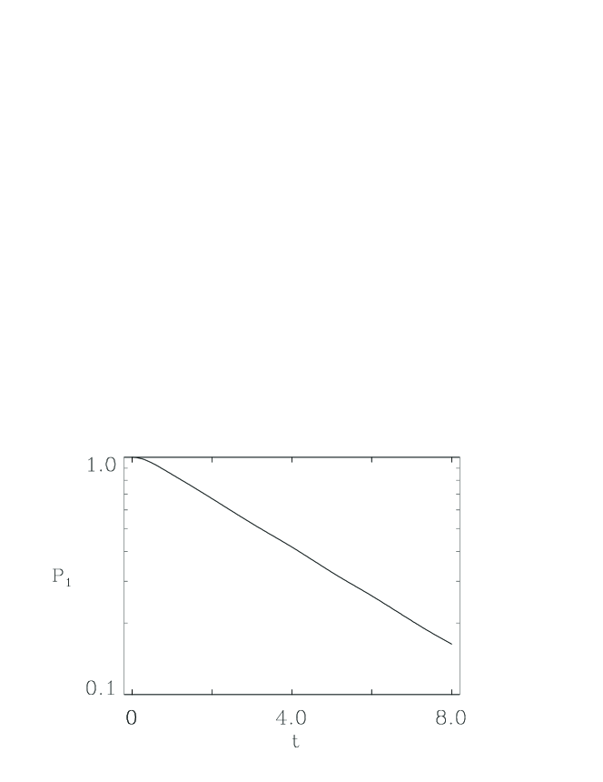
Figure 5: The system is prepared on the ground state of the harmonic potential, and the probability that it remains there is plotted as a function of time. The probability leaves the level in an exponential manner as this semilogarithmic plot shows.

In this paper we have reviewed the scattering theory approach to partitioning of the Hamiltonian time evolution in a quantum system. We are especially interested in the situation where one (or more) discrete states leak into a continuum, i.e., decay of quasistationary states. By choosing a Laplace-Fourier transform in time, we concentrate on solving an initial value problem and following the system as it irreversibly transfers its probability into the continuum. This is regarded as a wave packet preparation procedure.

The emphasis on time evolution has been motivated by the recent experimental progress in pulsed laser technology. It is now possible to excite a single state selectively, control its coupling to other states, including continuum ones, and follow the ensuing time evolution of the quantum states. Such work has experienced tremendous progress in molecular investigations recently, but also time resolved spectroscopy of semiconductor structures is possible.

Starting from a giving initial time, the future evolution of quantum systems is determined by the analytic properties of the propagator functions in the complex frequency plane. In order to obtain the correct physical behaviour these have to be continued analytically to a second Riemann sheet in the lower half plane. Any pole encountered will give rise to a resonance but the physical behaviour must also receive contributions from unavoidable branch cuts.

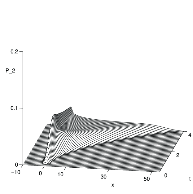
Figure 6: The probability $|\psi_{2}(x,t)|^{2}$ leaving the bound oscillator state appears on the sloping continuum potential. Here we can see it appear and fall down the slope in the form of a spreading wave packet. Part of the probability gets captured near the position of the original bound state because of trapping in the potential well formed by the adiabatic levels. This contains a component on the continuous manifold, which explains the trapped portion. Even this must eventually leave the trap but clearly over a much longer time scale.

The necessary analytic continuation introduces simple relations between the self-energy function in the upper half-plane and that in the lower. In the weak coupling limit, the Weisskopf-Wigner case, the prescription for continuation is found to be equivalent with adding a small dissipative mechanism to the states in the continuum. The causality requirement on the sign of this dissipation automatically affects the necessary analytic continuation. Physically we can understand this as follows: When probability leaks into the continuum through the weak coupling link, it is dissipated by all modes and oozes into the unobserved degrees of freedom providing the continuum damping. In scattering theory this mechanism is simply the outgoing boundary condition at infinity; all scattered modes are irreversibly lost at the edges of our universe. The bottle neck is provided by the weak link, and the rate of loss of the initial state is fixed by this. The dissipation in the continuum is only present to prevent any return of probability. Hence its details are inessential to the decay, its presence however is necessary.

We have discussed the analytic behaviour of the propagators in detail, and illustrate the properties by simple model calculations. Most of the treatment follows the tradition in this field and carries out the argument in the energy representation. However, to prove the existence of the phenomena discussed, we display the behaviour of a model describing laser coupling of a bound molecular state into a dissociating continuum. In addition to showing the expected exponential decay, the model system proves that the state prepared on the continuum is in the form of an outgoing wave packet. The model, however, also displays features not simply describable in the model calculations performed in this paper; we will return to a detailed exploration of the decay characteristics in a forthcoming publication.

The purpose of this paper is to draw attention to the necessity to investigate the time evolution in coupled quantum systems. This provides a broad range of interesting quantum models, which may also shed light on the phenomena occurring in dynamical processes initiated and explored by pulsed lasers.

Appendix

The algebraic manipulations we need in this paper have been provided by scattering theory long ago [7]. Here we summarize the main results only.

The perturbation series for the propagator is generated by the relation

$$G=G_{0}+G_{0}VG.$$ (A.1)

Introducing the operator $T$ by the relation

$$VG=TG_{0},$$ (A.2)

we find the equation

$$G=G_{0}+G_{0}TG_{0}.$$ (A.3)

The operator $T$ is obtained from the equation

$$T=V+TG_{0}V.$$ (A.4)

The disconnected operator $\Gamma$ is defined by the relation

$$\Gamma=V+VG_{0}^{Q}\Gamma,$$ (A.5)

where the projector $Q=1-P$ has been introduced. The missing singularities in the intermediate states can be reintroduced to get the $T$ operator

$$T=\Gamma+TG_{0}^{P}\Gamma.$$ (A.6)

When we remember the projectors commute with $H,$ we can easily solve

$$T^{P}=\Gamma^{P}\left(\frac{1}{1-G_{0}^{P}\Gamma^{P}}\right)$$ (A.7)

and

$$\begin{array}[]{ccc}G^{P}&=&G_{0}^{P}\left(1+T^{P}G_{0}^{P}\right)\\ &&\\ &=&\left(\frac{1}{\left(G_{0}^{p}\right)^{-1}-\Gamma^{P}}\right).\end{array}$$ (A.8)

In the same way we can calculate $G^{QP}$ from Eq. (A.1) and $G^{Q}$ from Eq. (A.3). The results are given in Eqs. (2.13) and (2.14).

These results are all exact, and they can be used to solve for the propagators of any Hamiltonian split into $H_{0}$ and $V$ and partitioned by projectors $P$ and $Q$ which separate the Hilbert space into subspaces not coupled by $V$.

References

- [1] L. D. Landau, Z. Physik. 45, 430 (1927).
- [2] V. Weisskopf and E. Wigner, Z. Physik. 63, 54 (1930).
- [3] V. Glaser and G. Källén, Nuclear Physics, 706 (1956).
- [4] R. E. Peierls, p. 296 in Proceedings of the 1954 Glasgow Conference (Pergamon Press, New York, 1955).
- [5] B. Zumino, p. 27 in Lectures on Field Theory and the Many-Body Problem, ed. E. R. Caianello (Academic Press, New York, 1961).
- [6] M. Levy, p. 47 in Lectures on Field Theory and the Many-Body Problem, ed. E. R. Caianello (Academic Press, New York, 1961).
- [7] M. L. Goldberger and K. M. Watson, Collision Theory, Chapter 8 (J. Wiley & Sons, New York, 1964).
- [8] L. Mower, Phys. Rev. 142, 799 (1966).
- [9] P. V. Ruuskanen, Nuclear Physics B22, 253 (1970).
- [10] J. Jortner, S. A. Rice and R. M. Hochstrasser, p. 149 in Advances in Photochemistry, Vol.7, eds. J. N. Pitts, Jr., G. S. Hammond, and W. A. Noyes, Jr. (Interscience, New York, 1969).
- [11] M. Gruebele and A. H. Zewail, Physics Today, p. 24, May 1990.
- [12] B. M. Garraway and K.-A. Suominen, Rep. Prog. Phys. 58, 365 (1995).
- [13] S. Stenholm and M. Kira, Acta Physica Slovaca 46, 325 (1996).
- [14] R. Peierls, More Surprises in Theoretical Physics, Sec. 5.3 (Princeton Univ. Press, Princeton, 1991).
- [15] G. Alber and P. Zoller, Phys. Rep. 199, 231 (1991).
- [16] M. Nauenberg, C. Stroud, and J. Yeazell, Scientific American, June 1994, p. 24.
- [17] C. Weissbuch and B. Winter, Quantum Semiconductor Structures, (Academic Press, New York, 1991) .
- [18] B. M. Garraway, to be published.
- [19] B. M. Garraway, private communication.
- [20] C. Cohen-Tannoudji, J. Dupont-Roc and G. Grynberg, Atom-Photon Interactions: Basic Principles and Applications, p. 239 (Wiley-Interscience, New York, 1992).
- [21] P. C. Martin, p. 37 in Many-Body Physics, Les Houches 1967, eds. B. DeWitt and R. Bailian (Gordon and Breach, New York, 1968).