Quantum harmonic oscillator state
synthesis and analysis

Abstract

We laser-cool single beryllium ions in a Paul trap to the ground $(n=0)$ quantum harmonic oscillator state with greater than 90% probability. From this starting point, we can put the atom into various quantum states of motion by application of optical and rf electric fields. Some of these states resemble classical states (the coherent states), while others are intrinsically quantum, such as number states or squeezed states. We have created entangled position and spin superposition states (Schrödinger cat states), where the atom’s spatial wavefunction is split into two widely separated wave packets. We have developed methods to reconstruct the density matrices and Wigner functions of arbitrary motional quantum states. These methods should make it possible to study decoherence of quantum superposition states and the transition from quantum to classical behavior. Calculations of the decoherence of superpositions of coherent states are presented.

Keywords: quantum state generation, quantum state tomography, laser cooling, ion storage, quantum computation

1. INTRODUCTION

In a series of studies we have prepared single, trapped, ⁹Be⁺ ions in various quantum harmonic oscillator states and performed measurements on those states. In this article, we summarize some of the results. Further details are given in the original reports [1, 2, 3, 4, 5].

The quantum states of the simple harmonic oscillator have been studied since the earliest days of quantum mechanics. For example, the harmonic oscillator was among the first applications of the matrix mechanics of Heisenberg [6] and the wave mechanics of Schrödinger [7]. The theoretical interest in harmonic oscillators is partly due to the fact that harmonic oscillator problems often have exact solutions. In addition, physical systems, such as vibrating molecules, mechanical resonators, or modes of the electromagnetic field, can be modeled as harmonic oscillators, so that the theoretical results can be compared to experiments.

A single ion in a Paul trap can be described effectively as a simple harmonic oscillator, even though the Hamiltonian is actually time-dependent, so no stationary states exist. For practical purposes, the system can be treated as if the Hamiltonian were that of an ordinary, time-independent harmonic oscillator (see, e.g., Refs. [8, 9]).

2. SYSTEM AND EFFECTIVE HAMILTONIAN

The effective Hamiltonian for the center-of-mass secular motion is that of an anisotropic three-dimensional harmonic oscillator. If we choose an interaction Hamiltonian which affects only the $x$-motion, then we can deal with the one-dimensional harmonic oscillator Hamiltonian,

$$H_{x}=\hbar\omega_{x}a_{x}^{\dagger}a_{x},$$ (1)

where $\omega_{x}$ is the secular frequency for the $x$-motion, and $a_{x}^{\dagger}$ and $a_{x}$ are the creation and annihilation operators for the quanta of the $x$-oscillation mode. The constant term $\hbar\omega_{x}/2$, which results from the usual quantization procedure, has been left out for convenience. The eigenstates of $H_{x}$ are $|n_{x}\rangle$, where

$$H_{x}|n_{x}\rangle=n_{x}\hbar\omega_{x}|n_{x}\rangle.$$ (2)

The internal states of the ⁹Be⁺ ion which are the most important for the experiments are shown in Fig. 1. We are mostly concerned with the hyperfine-Zeeman sublevels of the ground $2s\,^{2}S_{1/2}$ electronic state, which are denoted by $|2s\,^{2}S_{1/2};F,M_{F}\rangle$, where ${\bf F}$ is the total angular momentum, and $M_{F}$ is the eigenvalue of $F_{z}$. The ⁹Be nucleus has spin 3/2. Of chief importance are $|2s\,^{2}S_{1/2};2,2\rangle$, abbreviated as $|\!\downarrow\rangle$, and $|2s\,^{2}S_{1/2};1,1\rangle$, abbreviated as $|\!\uparrow\rangle$. The hyperfine-Zeeman sublevels of the $2p\,^{2}P_{J}$ ($J=1/2$ or $3/2$) fine-structure multiplet also play a role, either as intermediate states in stimulated Raman transitions or as the final states in resonantly-driven single-photon transitions used for laser cooling or state detection. We denote these states by $|2p\,^{2}P_{J};F,M_{F}\rangle$. The energy separation of $|\!\uparrow\rangle$ and $|\!\downarrow\rangle$ is $\hbar\omega_{0}$, where $\omega_{0}\approx 2\pi\times 1.250$ GHz. They are coupled by laser beams R1 and R2, through the intermediate $|2p\,^{2}P_{1/2};2,2\rangle$ state. The frequency detuning from the intermediate state is $\Delta$, where $\Delta\approx-2\pi\times 12$ GHz.

If we restrict the internal states to the space spanned by $|\!\uparrow\rangle$ and $|\!\downarrow\rangle$, then the internal Hamiltonian can be written as

$$H_{\uparrow\downarrow}=\frac{\hbar\omega_{0}}{2}\sigma_{z},$$ (3)

where $\sigma_{z}$ is a Pauli spin matrix whose nonzero matrix elements are$\langle\uparrow\!|\sigma_{z}|\!\uparrow\rangle=+1$ and $\langle\downarrow\!|\sigma_{z}|\!\downarrow\rangle=-1$.

Figure 1: Internal and motional energy levels of a ⁹Be⁺ ion. The $|\!\uparrow\rangle$ and $|\!\downarrow\rangle$ states are particular hyperfine-Zeeman components of the ground ${}^{2}S_{1/2}$ state, separated in energy by $\hbar\omega_{0}$. Each internal state can exist in any of a ladder of vibrational energy states $|n_{x}\rangle$, where $n_{x}=0,1,2,\ldots$, separated in energy by $\hbar\omega_{x}$, where $\omega_{x}\approx 2\pi\times 11.2$ MHz.

The total effective Hamiltonian for the system consisting of the internal $|\!\uparrow\rangle$ and $|\!\downarrow\rangle$ states and the $x$ motional degree of freedom is

$$H=H_{\uparrow\downarrow}+H_{x}+H_{\rm int},$$ (4)

where $H_{\rm int}$ is the effective interaction Hamiltonian coupling due to the two laser beams R1 and R2 in Fig. 1. We define an interaction-picture operator ${\cal O}^{I}$ in terms of a Schrödinger-picture operator ${\cal O}^{S}$ as

$${\cal O}^{I}(t)=e^{iH_{\uparrow\downarrow}t/\hbar}{\cal O}^{S}(t)e^{-iH_{\uparrow\downarrow}t/\hbar}.$$ (5)

The effective interaction Hamiltonian in the interaction picture and the rotating wave approximation is

$$H^{I}_{\rm int}=\hbar g\left(\sigma_{+}e^{i\eta(a_{x}^{\dagger}+a_{x})-i\delta t}+\sigma_{-}e^{-i\eta(a_{x}^{\dagger}+a_{x})+i\delta t}\right),$$ (6)

where $g$ is the interaction strength, $\delta$ is the detuning of the frequency difference of the two laser beams with respect to $\omega_{0}$, and $\eta=k\sqrt{\hbar/(2m\omega_{x})}$ is the Lamb-Dicke parameter, where $k$ is the magnitude of the difference between the wavevectors of the two laser beams, and $m$ is the mass of the ion. The nonzero matrix elements of $\sigma_{+}$ and $\sigma_{-}$ are $\langle\uparrow\!|\sigma_{+}|\!\downarrow\rangle=\langle\downarrow\!|\sigma_{-}|\!\uparrow\rangle=1$.

The detuning $\delta$ can be tuned to multiples of $\omega_{x}$, $\delta=(n^{\prime}-n)\omega_{x}$, so as to resonantly drive transitions between $|\!\downarrow,n\rangle$ and $|\!\uparrow,n^{\prime}\rangle$. We refer to the $\delta=0$ resonance as the carrier, the $\delta=-\omega_{x}$ resonance as the first red sideband, and the $\delta=+\omega_{x}$ resonance as the first blue sideband.

The signal that is detected in the experiments is the probability
                                                                $P_{\downarrow}(t)$ that the ion is in the $|\!\!\downarrow\rangle$ internal state after a particular preparation. If we irradiate the ion at time $t$ with circularly polarized light, resonant with the electronic transition from $|\!\downarrow\rangle$ to $|2p\,^{2}P_{3/2};3,3\rangle$, there will be a high fluorescence intensity if the $|\!\downarrow\rangle$ state is occupied, since the selection rules only allow that upper state to decay back to the $|\!\downarrow\rangle$ state, so it can continue to scatter photons. This transition is called a cycling transition. If the ion is in the $|\!\uparrow\rangle$ state when it is irradiated with the same light, it will scatter a negligible number of photons. Thus, if we repeatedly prepare the ion in the same way, apply radiation resonant with the cycling transition, and detect the fluorescence photons, the average signal will be proportional to $P_{\downarrow}(t)$.

3. CREATION AND PARTIAL MEASUREMENTS OF QUANTUM STATES

3.1. Fock states

The ion is prepared in the $n=0$ state by Raman cooling [1]. (From now on we drop the $x$ label on $n$.) Raman cooling consists of a sequence of laser pulses on the red sideband, driving $|\!\downarrow,n\rangle$ to $|\!\uparrow,n-1\rangle$ transitions, followed by laser pulses which recycle the ion back to the $|\!\downarrow,n-1\rangle$ state. The probability of heating due to recoil during the recycling step is small. At the end of the sequence, the ion is in the $n=0$ state more than 90% of the time.

A Fock state is another name for an $n$-state. Higher-$n$ Fock states are prepared from the $n=0$ state by a sequence of $\pi$-pulses on the blue sideband, red sideband, or carrier. For example, the $|\!\uparrow,2\rangle$ state is prepared by using blue sideband, red sideband, and carrier $\pi$-pulses in succession, so that the ion steps through the states $|\!\downarrow,0\rangle$, $|\!\uparrow,1\rangle$, $|\!\downarrow,2\rangle$, and $|\!\uparrow,2\rangle$.

If the atom is initially in the $|\!\downarrow,n\rangle$ state, and the first blue sideband is driven, it will oscillate between that state and the $|\!\uparrow,n+1\rangle$ state. The probability of finding it in the $|\!\downarrow,n\rangle$ state at a time $t$ is

$$P_{\downarrow}(t)=\frac{1}{2}\left[1+\cos(2\Omega_{n,n+1}t)e^{-\gamma_{n}t}\right],$$ (7)

where $\Omega_{n,n+1}$, the Rabi flopping rate, is a function of the laser intensities and detunings and $n$, and $\gamma_{n}$ is a damping factor which is determined empirically. Thus, the frequency of the oscillations of $P_{\downarrow}(t)$ is a signature of the initial value of $n$. Figure 2(a) shows $P_{\downarrow}(t)$ for an initial $|\!\downarrow,0\rangle$ state. Figure 2(b) shows the observed ratios of Rabi frequencies compared with the values calculated from the matrix elements of the interaction Hamiltonian [Eq. (6)].

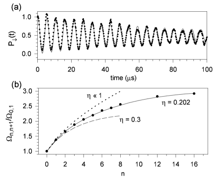
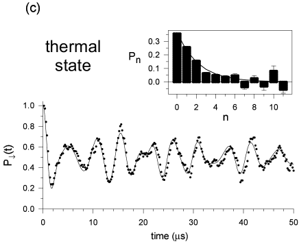
Figure 2: (a) $P_{\downarrow}(t)$ for an initial $|\!\downarrow,0\rangle$ number state driven by the first blue sideband. The solid line is a fit to an exponentially damped sinusoid. (b) Observed ratios of the Rabi frequencies $\Omega_{n,n+1}/\Omega_{0,1}$ for different values of the initial $n$. The lines represent calculated values for different values of the Lamb-Dicke parameter $\eta$. The value of $\eta$, inferred from other measured quantities, was $0.202\pm 0.005$. (c) $P_{\downarrow}(t)$ for a thermal state. The solid line is a fit of the data (dots) to a sum of Fock states having a thermal distribution. The fitted value for the mean value of $n$ is $\overline{n}=1.3\pm 0.1$. The inset shows the amplitudes of the Fock state components (bars) with a fit to an exponential, corresponding to $\overline{n}=1.5\pm 0.1$ (line).

3.2. Thermal states

A thermal state of the motion of the ion is not a pure state, but rather must be described by a density matrix, even though there is only one ion. The statistical ensemble which is described by the density matrix is generated by repeatedly preparing the state and making a measurement.

The ion is prepared in a thermal state by Doppler laser cooling [10]. The temperature of the distribution can be controlled by changing the detuning of the cooling laser. When the ion’s state is not a Fock state, $P_{\downarrow}(t)$ has the form

$$P_{\downarrow}(t)=\frac{1}{2}\left[1+\sum_{n=0}^{\infty}P_{n}\cos(2\Omega_{n,n+1}t)e^{-\gamma_{n}t}\right],$$ (8)

where $P_{n}$ is the probability of finding the ion in the state $|n\rangle$. Figure 2(c) shows $P_{\downarrow}(t)$ for a thermal state.

3.3. Coherent states

Coherent states of the quantum harmonic oscillator were introduced by Schrödinger [11], with the aim of describing a classical particle with a wavefunction. A coherent state $|\alpha\rangle$ is equal to the following superposition of number states:

$$|\alpha\rangle=e^{-\frac{1}{2}{|\alpha|}^{2}}\sum_{n=0}^{\infty}\frac{\alpha^{n}}{\sqrt{n!}}|n\rangle.$$ (9)

In the Schrödinger picture, the absolute square of the wavefunction retains its shape, and its center follows the trajectory of a classical particle in a harmonic well. The mean value of $n$ is $\overline{n}=|\alpha|^{2}$. A coherent state can be created from the $n=0$ state (a special case of coherent state) by applying a spatially uniform classical force (see Appendix A). The drive is most effective when its frequency is $\omega_{x}$. Another method is to apply a “moving standing wave,” that is, two laser beams differing in frequency by $\omega_{x}$ and differing in propagation direction, so that an oscillating dipole force is generated [12]. We have used both of these methods to prepare coherent states. Figure 3(a) shows $P_{\downarrow}(t)$ for a coherent state. This trace exhibits the phenomenon of collapse and revival [13].

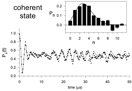
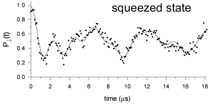
Figure 3: (a) $P_{\downarrow}(t)$ for a coherent state. The solid line is a fit of the data (dots) to a sum of Fock states having a coherent state distribution. The fitted value for $\overline{n}$ is $3.1\pm 0.1$. The inset shows the amplitudes of the Fock state components (bars) with a fit to a Poissonian distribution, corresponding to $\overline{n}=2.9\pm 0.1$ (line). (b) $P_{\downarrow}(t)$ for a squeezed state. The solid line is a fit of the data (dots) to a sum of Fock states having a squeezed-state distribution. The fitted value for $\beta$ is $40\pm 10$, which corresponds to $\overline{n}\approx 7.1$

3.4. Squeezed states

Figure 4: Creation of a Schrödinger cat state. See text for details.

A “vacuum squeezed state” can be created by applying an electric field gradient having a frequency of $2\omega_{x}$ to an ion initially in the $n=0$ state [14]. Here, the ion was irradiated with two laser beams which differed in frequency by $2\omega_{x}$. This has the same effect. The squeeze parameter $\beta$ is defined as the factor by which the variance of the squeezed quadrature is decreased. It increases exponentially with the time the driving force is applied. The probability distribution of $n$-states is nonzero only for even $n$, for which,

$$P_{2n}=N\frac{(2n)!(\tanh r)^{2n}}{(2^{n}n!)^{2}},$$ (10)

where $\beta=e^{2r}$, and $N$ is a normalization constant. Figure 3(b) shows $P_{\downarrow}(t)$ for a squeezed state having $\beta=40\pm 10$.

3.5. Schrödinger cat states

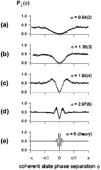
Figure 5: Measured and fitted $P_{\downarrow}(\phi)$ interference signals for the Schrödinger cat state. The curves in (a) through (d) represent measurements for different values of the time during which the displacement beams excite the coherent states. The solid lines are fits to Eq. (12), allowing $\alpha$ to vary. In (d), a term representing loss of contrast was included in the fit. The curve in (d) represents a superposition of two $x_{0}\approx 7$ nm wave packets with a maximum separation of $4\alpha x_{0}\approx 80$ nm. Curve (e) represents a calculation for a pair of coherent states with $\alpha=6$.

The term “Schrödinger cat” is taken here to denote an entangled state which consists of two coherent states of motion correlated with different internal atomic states. A simple example is

$$|\Psi\rangle=\frac{|\!\uparrow,\alpha\rangle+|\!\downarrow,-\alpha\rangle}{\sqrt{2}}.$$ (11)

Figure 4 shows how such a state is created. (a) The ion is prepared in the $|\!\downarrow,0\rangle$ state by Raman cooling. (b) A $\pi/2$-pulse on the carrier generates an equal superposition of $|\!\downarrow,0\rangle$ and $|\!\uparrow,0\rangle$. (c) The displacement beams generate a force ${\bf F_{1}}$, which excites the component in the $|\!\uparrow\rangle$ internal state to a coherent state $|\alpha\rangle$. Due to the polarizations of the displacement beams, they do not affect an atom in the $|\!\downarrow\rangle$ state. (d) A $\pi$-pulse on the carrier exchanges the $|\!\downarrow\rangle$ and $|\!\uparrow\rangle$ components. (e) The displacement beams generate a force ${\bf F_{2}}$, which excites the component in the $|\!\uparrow\rangle$ internal state to a coherent state $|\alpha e^{i\phi}\rangle$, where the phase $\phi$ is controlled by an rf oscillator. The state here is analogous to Schrödinger’s cat. (f) The $|\!\downarrow\rangle$ and $|\!\uparrow\rangle$ components are combined by a $\pi/2$-pulse on the carrier. At this point, the radiation is applied on the cycling transition, and the signal is recorded.

The predicted signal, for a particular value of $\phi$, is

$$P_{\downarrow}(\phi)=\frac{1}{2}\left[1-ce^{-\alpha^{2}(1-\cos\phi)}\cos(\alpha^{2}\sin\phi)\right],$$ (12)

where $c=1$ in the absence of decoherence. Figure 5 shows experimental data and fits to Eq. (12) for various values of $\alpha$. In (d), $c$ is clearly less than one, indicating decoherence, although the source is not yet determined.

4. COMPLETE MEASUREMENTS OF QUANTUM STATES

The measurements described in the previous Section determine only the $n$-state populations or probabilities, and therefore do not provide a complete description of the motional states. The density matrix $\rho$ does provide a complete description of a state, whether it is a pure or a mixed state. The Wigner function $W(\alpha)$ also provides a complete description. The Wigner function resembles a classical joint probability distribution for position and momentum in some cases. However, it can be negative, unlike a true probability distribution. We have demonstrated experimental methods for reconstructing the density matrix or the Wigner function of a quantum state of motion of a harmonically bound atom [4].

Both of these methods depend on controllably displacing the state in phase space, applying radiation to drive the first blue sideband for time $t$, and then measuring $P_{\downarrow}$. The averaged, normalized, signal is

$$P_{\downarrow}(t,\alpha)=\frac{1}{2}\left[1+\sum_{k=0}^{\infty}Q_{k}(\alpha)\cos(2\Omega_{k,k+1}t)e^{-\gamma_{k}t}\right],$$ (13)

where the complex number $\alpha$ represents the amplitude and phase of the displacement, and $Q(\alpha)$ is the occupation probability of the vibrational state $|k\rangle$ for the displaced state.

If the $Q_{k}(\alpha)$ coefficients are derived for a series of values of $\alpha$ lying in a circle,

$$\alpha_{p}=|\alpha|\exp[i(\pi/N)p],$$ (14)

where $p=-N,\ldots,N-1$, then the density matrix elements $\rho_{nm}$ can be determined for values of $n$ and $m$ up to $N-1$. The details of the numerical procedure are given in Ref. [4].

Figure 6(a) shows the reconstructed density matrix amplitudes for an approximate $n=1$ state. Figure 6(b) shows the reconstructed density matrix for a coherent state having an amplitude $|\beta|\approx 0.67$.

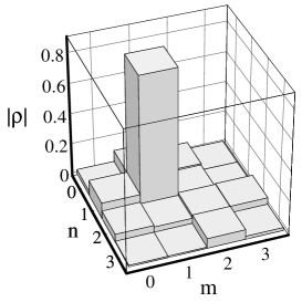
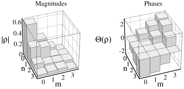
Figure 6: (a) Reconstructed number-state density matrix amplitudes $|\rho_{nm}|$ for an approximate $n=1$ number state. (b) Reconstructed amplitudes $|\rho_{nm}|$ and phases $\Theta(\rho_{nm})$ of a coherent state.

The Wigner function for a given value of the complex parameter $\alpha$ can be determined from the sum [15, 16, 17, 18]

$$W(\alpha)=\frac{2}{\pi}\sum_{n=0}^{\infty}(-1)^{n}Q_{n}(\alpha).$$ (15)

Figure 7 shows the reconstructed Wigner function for an approximate $n=1$ state. The fact that it is negative in a region around the origin highlights the fact that is a nonclassical state. Figure 8 shows the reconstructed Wigner function for a coherent state with amplitude $|\beta|\approx 1.5$. It is positive, which is not surprising, since the coherent state is the quantum state that most closely approximates a classical state.

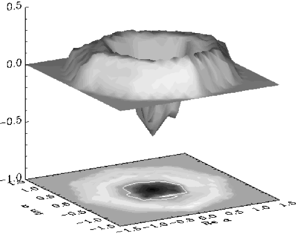
Figure 7: Surface and contour plots of the reconstructed Wigner function $W(\alpha)$ of an approximate $n=1$ number state. The negative values of $W(\alpha)$ around the origin highlight the nonclassical nature of this state.

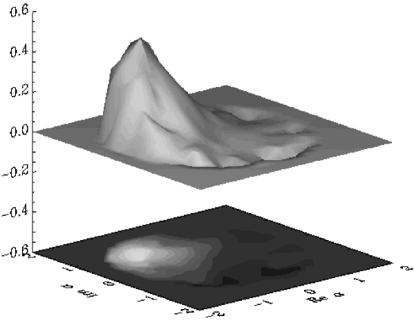
Figure 8: Surface and contour plots of the reconstructed Wigner function $W(\alpha)$ of a coherent state. The width is in good agreement with the expected minimum-uncertainty value.

5. DECOHERENCE OF A SUPERPOSITION OF COHERENT STATES

Decoherence, the decay of superposition states into mixtures, is of interest because it leads to the familiar classical physics of macroscopic objects (see, e.g. Ref. [19]). Experiments are beginning to probe the regime in which decoherence is observable, but not so fast that the dynamics are classical. One example is the observation of the decoherence of a superposition of mesoscopic (few-photon) quantum states of an electromagnetic field having distinct phases by Brune et al. [20] In this experiment, as in the Schrödinger cat experiment of Ref. [3], the mesoscopic system was entangled with an internal two-level system of an atom.

A simpler system, which has been well-studied theoretically by others [21, 22, 23, 24], is a superposition of two coherent states of a harmonic oscillator, without entanglement with a two-level system. The system interacts in some way with the environment, leading to decoherence of the superposition state.

Here we carry out a simple calculation of the decoherence of a superposition of two coherent states of a harmonic oscillator. At time $t=0$, the system is in an equal superposition of two coherent states,

$$|\Psi(0)\rangle=\frac{1}{\sqrt{2}}\left(e^{i\theta_{1}(0)}|\alpha_{1}(0)\rangle+e^{i\theta_{2}(0)}|\alpha_{2}(0)\rangle\right),$$ (16)

where the notation is the same as in Appendix A, and the interaction picture is used. (It is assumed that the two components of the state vector are nearly orthogonal. Otherwise the normalization factor is different.) The system is subjected to a random force, which is uniform over the spatial extent of the system, for example, a uniform electric field acting on a charged particle. In Appendix A, we show that a single coherent state, subjected to such a force, will remain in a coherent state. It follows from the linearity of the Schrödinger equation that the state described by Eq. (16) will, at a later time, still be in an equal superposition of coherent states, although $\alpha_{1}$, $\alpha_{2}$, $\theta_{1}$, and $\theta_{2}$ will change. Each time the system of Eq. (16) is prepared, $\alpha_{1}$, $\alpha_{2}$, $\theta_{1}$, and $\theta_{2}$ will have a different time dependence, due to the random force. We can study the decoherence as a function of time by carrying out an ensemble average.

Although both $\alpha_{1}$ and $\alpha_{2}$ change with time, their difference does not, since they each change by the same amount. This can be seen from Eq. (45). We define $\Delta\alpha\equiv\alpha_{1}-\alpha_{2}={\rm constant}$.

Decoherence is due to the changes in the phase difference $[\theta_{2}(t)-\theta_{1}(t)]$. We define the change in the phase difference to be

$$\Delta\theta(t)\equiv[\theta_{2}(t)-\theta_{1}(t)]-[\theta_{2}(0)-\theta_{1}(0)].$$ (17)

Then, from Eq. (48),

$$\Delta\theta(t)=\frac{1}{2}\left[\Delta\alpha\int_{0}^{t}f(t^{\prime})e^{-i\omega_{x}t^{\prime}}dt^{\prime}+\Delta\alpha^{*}\int_{0}^{t}f(t^{\prime})e^{i\omega_{x}t^{\prime}}dt^{\prime}\right].$$ (18)

The double-integral term in Eq. (48) does not contribute to $\Delta\theta(t)$, since it does not depend on either $\alpha(0)$ or $\theta(0)$, so it makes the same contribution to $\theta_{2}(t)$ and to $\theta_{1}(t)$. The square of $\Delta\theta(t)$ is

$$\left(\Delta\theta(t)\right)^{2} = \frac{1}{4}\left[(\Delta\alpha)^{2}\int_{0}^{t}\int_{0}^{t}f(t^{\prime})f(t^{\prime\prime})e^{-i\omega_{x}t^{\prime}-i\omega_{x}t^{\prime\prime}}dt^{\prime}dt^{\prime\prime}+2|\Delta\alpha|^{2}\int_{0}^{t}\int_{0}^{t}f(t^{\prime})f(t^{\prime\prime})e^{i\omega_{x}t^{\prime}-i\omega_{x}t^{\prime\prime}}dt^{\prime}dt^{\prime\prime}\right.$$ (19)

$$\left.\mbox{}+(\Delta\alpha^{*})^{2}\int_{0}^{t}\int_{0}^{t}f(t^{\prime})f(t^{\prime\prime})e^{i\omega_{x}t^{\prime}+i\omega_{x}t^{\prime\prime}}dt^{\prime}dt^{\prime\prime}\right],$$

and its ensemble average is

$$\left\langle\left(\Delta\theta(t)\right)^{2}\right\rangle = \frac{1}{4}\left[(\Delta\alpha)^{2}\int_{0}^{t}\int_{0}^{t}\langle f(t^{\prime})f(t^{\prime\prime})\rangle e^{-i\omega_{x}t^{\prime}-i\omega_{x}t^{\prime\prime}}dt^{\prime}dt^{\prime\prime}+2|\Delta\alpha|^{2}\int_{0}^{t}\int_{0}^{t}\langle f(t^{\prime})f(t^{\prime\prime})\rangle e^{i\omega_{x}t^{\prime}-i\omega_{x}t^{\prime\prime}}dt^{\prime}dt^{\prime\prime}\right.$$ (20)

$$\left.\mbox{}+(\Delta\alpha^{*})^{2}\int_{0}^{t}\int_{0}^{t}\langle f(t^{\prime})f(t^{\prime\prime})\rangle e^{i\omega_{x}t^{\prime}+i\omega_{x}t^{\prime\prime}}dt^{\prime}dt^{\prime\prime}\right],$$

where the angular brackets denote an ensemble average. Thus, $\left\langle\left(\Delta\theta(t)\right)^{2}\right\rangle$ depends on the autocorrelation function of the random function $f(t)$, which is proportional to the force. If we assume that $f$ is a stationary random variable, then its autocorrelation function

$$R(\tau)=\langle f(t)f(t+\tau)\rangle$$ (21)

exists and is independent of $t$. According to the Wiener-Khinchine theorem, the power spectrum $w(\nu)$, defined for $\nu\geq 0$, is

$$w(\nu)=4\int_{0}^{\infty}R(\tau)\cos(2\pi\nu\tau)d\tau.$$ (22)

A white-noise spectrum corresponds to $R(\tau)\propto\delta(\tau)$, where $\delta(\tau)$ is the Dirac delta function. If we let $R(\tau)=C\delta(\tau)$, then

$$\left\langle\left(\Delta\theta(t)\right)^{2}\right\rangle = \frac{C}{4}\left[(\Delta\alpha)^{2}\int_{0}^{t}\int_{0}^{t}\delta(t^{\prime\prime}-t^{\prime})e^{-i\omega_{x}t^{\prime}-i\omega_{x}t^{\prime\prime}}dt^{\prime}dt^{\prime\prime}+2|\Delta\alpha|^{2}\int_{0}^{t}\int_{0}^{t}\delta(t^{\prime\prime}-t^{\prime})e^{i\omega_{x}t^{\prime}-i\omega_{x}t^{\prime\prime}}dt^{\prime}dt^{\prime\prime}\right.$$ (23)

$$\left.\mbox{}+(\Delta\alpha^{*})^{2}\int_{0}^{t}\int_{0}^{t}\delta(t^{\prime\prime}-t^{\prime})e^{i\omega_{x}t^{\prime}+i\omega_{x}t^{\prime\prime}}dt^{\prime}dt^{\prime\prime}\right]$$

$$= \frac{C}{4}\left[(\Delta\alpha)^{2}\int_{0}^{t}e^{-2i\omega_{x}t^{\prime}}dt^{\prime}+2|\Delta\alpha|^{2}\int_{0}^{t}dt^{\prime}+(\Delta\alpha^{*})^{2}\int_{0}^{t}e^{2i\omega_{x}t^{\prime}}dt^{\prime}\right].$$

The first and third integrals on the right-hand-side of Eq. (23) oscillate, but are bounded, while the second one grows with time, so, for $\omega_{x}t\gg 1$,

$$\left\langle\left(\Delta\theta(t)\right)^{2}\right\rangle\approx\frac{1}{2}C|\Delta\alpha|^{2}t.$$ (24)

Hence, the decoherence time, that is, the time required for the rms phase difference $\left\langle\left(\Delta\theta(t)\right)^{2}\right\rangle^{1/2}$ to increase to about 1 radian, is on the order of $2/\left(C|\Delta\alpha|^{2}\right)$.

Using the same approximations, we can calculate the rate of change of the amplitude $\alpha_{i}(t)$ for a single coherent state, where $i$ is 1 or 2. From Eq. (45) in Appendix A,

$$\alpha_{i}(t)-\alpha_{i}(0)=i\int_{0}^{t}f(t^{\prime})e^{i\omega_{x}t^{\prime}}dt^{\prime},$$ (25)

and

$$|\alpha_{i}(t)-\alpha_{i}(0)|^{2}=\int_{0}^{t}\int_{0}^{t}f(t^{\prime})f(t^{\prime\prime})e^{i\omega_{x}t^{\prime}-i\omega_{x}t^{\prime\prime}}dt^{\prime}dt^{\prime\prime}.$$ (26)

If $f(t)$ has a white-noise spectrum, as considered previously, the ensemble average is

$$\left\langle|\alpha_{i}(t)-\alpha_{i}(0)|^{2}\right\rangle=C\int_{0}^{t}\int_{0}^{t}\delta(t^{\prime\prime}-t^{\prime})e^{i\omega_{x}t^{\prime}-i\omega_{x}t^{\prime\prime}}dt^{\prime}dt^{\prime\prime}=C\int_{0}^{t}dt^{\prime}=Ct.$$ (27)

In the time, $t\approx 2/\left(C|\Delta\alpha|^{2}\right)$, required for decoherence, the rms change in $\alpha_{i}$ is $\sqrt{2}/|\Delta\alpha|$. Consider the case $\alpha_{1}(0)=-\alpha_{2}(0)$. The energy of a single coherent state is proportional to the square of its amplitude ($\propto|\alpha_{i}|^{2}$). The fractional change in the energy is

$$\left|\frac{\Delta|\alpha_{i}|^{2}}{|\alpha_{i}|^{2}}\right|<\frac{2|\alpha_{i}(t)-\alpha_{i}(0)|}{\alpha_{i}(0)}\approx\frac{2\sqrt{2}}{|\Delta\alpha||\alpha_{i}(0)|}=\frac{\sqrt{2}}{|\alpha_{i}(0)|^{2}},$$ (28)

which becomes small for $|\alpha_{i}(0)|^{2}\gg 1$. Thus, we see that coherent superpositions of macroscopic ($|\alpha_{i}(0)|^{2}\gg 1$) states decohere much more quickly than they change in energy.

We can make a more quantitative statement about the decoherence rate by considering the decay of the off-diagonal density matrix elements. For an initial pure state $2^{-1/2}(|\alpha_{1}\rangle+|\alpha_{2}\rangle)$, the density matrix is

$$\rho=\frac{1}{2}\left(|\alpha_{1}\rangle\langle\alpha_{1}|+|\alpha_{1}\rangle\langle\alpha_{2}|+|\alpha_{2}\rangle\langle\alpha_{1}|+|\alpha_{2}\rangle\langle\alpha_{2}|\right).$$ (29)

If $\Delta\alpha\gg 1$, so that the phase changes are more important than the changes in $\alpha_{1}$ and $\alpha_{2}$, then the off-diagonal matrix element $|\alpha_{2}\rangle\langle\alpha_{1}|$ evolves to $e^{i\Delta\theta(t)}|\alpha_{2}\rangle\langle\alpha_{1}|$. Let us assume that the random variable $\Delta\theta$ at time $t$ has a Gaussian distribution $P(\Delta\theta)$. Given the variance of $\Delta\theta$ from Eq. (24), $P(\Delta\theta)$ must have the form

$$P(\Delta\theta)=\frac{1}{\sqrt{\pi C|\Delta\alpha|^{2}t}}\exp\left(-\frac{\Delta\theta^{2}}{C|\Delta\alpha|^{2}t}\right).$$ (30)

We evaluate the ensemble average of $e^{i\Delta\theta(t)}$,

$$\left\langle e^{i\Delta\theta(t)}\right\rangle=\int_{-\infty}^{\infty}P(\Delta\theta)e^{i\Delta\theta(t)}d(\Delta\theta)=\exp\left(-\frac{C|\Delta\alpha|^{2}t}{4}\right).$$ (31)

This yields the basic result, previously derived by others [21, 22, 23, 24], that the off-diagonal matrix element decays exponentially in time, with a time constant that is inversely proportional to $|\Delta\alpha|^{2}$.

An extension of the experiment of Ref. [3], with a random electric field deliberately applied, might be used to verify these calculations [3]. A means of simulating thermal, zero-temperature, squeezed, and other reservoirs by various combinations of optical fields has been discussed by Poyatos et al. [25]

APPENDIX A. THE FORCED HARMONIC OSCILLATOR

If a coherent state is subjected to a spatially uniform force, it remains a coherent state, though its amplitude changes. This exact result, which is independent of the strength or time-dependence of the force, seems to have been discovered by Husimi [26] and independently by Kerner [27]. For other references on the forced quantum harmonic oscillator, see Ref. [28]. The qualitative result stated above is enough to establish that applying a force to the $n=0$ state will generate a finite-amplitude coherent state, which was required in Sec. 3.3..   However, in order to study the decoherence of a superposition of two coherent states, it is useful to have an exact expression for the time-dependent state vector, given that the state vector is an arbitrary coherent state at $t=0$. Since the published results of which we are aware do not give this particular result, we give here an elementary derivation.

We consider a Hamiltonian, $H=H_{0}+V(t)$, where $H_{0}=\hbar\omega_{x}a_{x}^{\dagger}a_{x}$ is the Hamiltonian of a one-dimensional harmonic oscillator, and $V(t)=-xF(t)$ is a time-dependent potential. Here, $F(t)$ is a real $c$-number function of time and corresponds to a spatially uniform force, and $x=x_{0}(a_{x}+a_{x}^{\dagger})$, where $x_{0}\equiv(\hbar/2m\omega_{x})^{1/2}$. For example, if the particle has charge $q$, and a uniform electric field $\hat{x}E_{x}(t)$ is applied, then $F(t)=qE_{x}(t)$.

It is convenient to switch to the interaction picture, where an interaction-picture state vector $|\Psi(t)\rangle^{I}$ is related to the corresponding Schrödinger-picture state vector $|\Psi(t)\rangle^{S}$ by

$$|\Psi(t)\rangle^{I}=e^{iH_{0}t/\hbar}|\Psi(t)\rangle^{S},$$ (32)

and an interaction-picture operator ${\cal O}^{I}(t)$ is related to the corresponding Schrödinger-picture operator ${\cal O}^{S}(t)$ by

$${\cal O}^{I}(t)=e^{iH_{0}t/\hbar}{\cal O}^{S}(t)e^{-iH_{0}t/\hbar}.$$ (33)

The equation of motion for an interaction-picture operator is

$$\frac{d}{dt}{\cal O}^{I}(t)=-\frac{i}{\hbar}\left[{\cal O}^{I}(t),H_{0}\right],$$ (34)

so

$$\frac{d}{dt}a_{x}^{I}(t) = -\frac{i}{\hbar}\left[a_{x}^{I}(t),H_{0}\right]=-i\omega_{x}a^{I}(t),$$ (35)

$$a_{x}^{I}(t) = a_{x}^{I}(0)e^{-i\omega_{x}t},$$ (36)

$${a_{x}^{\dagger}}^{I}(t) = {a_{x}^{\dagger}}^{I}(0)e^{i\omega_{x}t}.$$ (37)

For simplicity, we let $a\equiv a_{x}^{I}(0)=a_{x}^{S}$ and $a^{\dagger}\equiv{a_{x}^{\dagger}}^{I}(0)={a_{x}^{\dagger}}^{S}$. The Schrödinger equation in the interaction picture is

$$\frac{\partial}{\partial t}|\Psi(t)\rangle^{I}=-\frac{i}{\hbar}V^{I}(t)|\Psi(t)\rangle^{I}=if(t)\left(ae^{-i\omega_{x}t}+a^{\dagger}e^{i\omega_{x}t}\right)|\Psi(t)\rangle^{I},$$ (38)

where $f(t)\equiv x_{0}F(t)/\hbar$. Note that if $f(t)=0$, $|\Psi(t)\rangle^{I}$ is constant.

We impose the initial condition that $|\Psi(0)\rangle^{I}$ is a coherent state. We make the assumption that $|\Psi(t)\rangle^{I}$ is also a coherent state for $t>0$,

$$|\Psi(t)\rangle^{I}=e^{i\theta(t)}|\alpha(t)\rangle\equiv e^{i\theta(t)}e^{-\frac{1}{2}|\alpha(t)|^{2}}\sum_{n=0}^{\infty}\frac{\alpha^{n}(t)}{\sqrt{n!}}|n\rangle,$$ (39)

where the $|n\rangle$ are the eigenstates of $a_{x}^{\dagger}a_{x}$ with eigenvalue $n$ at $t=0$, and $\theta(t)$ is an arbitrary real function, so that ${}^{I}\langle\Psi(t)|\Psi(t)\rangle^{I}=1$. (This assumption must be verified later by substitution of the resulting solution back into Eq. (38).) The problem reduces to finding the complex function $\alpha(t)$ and the real function $\theta(t)$.

The right-hand-side of Eq. (38) is

$$-\frac{i}{\hbar}V^{I}(t)|\Psi(t)\rangle^{I} = if(t)\left(ae^{-i\omega_{x}t}+a^{\dagger}e^{i\omega_{x}t}\right)e^{i\theta(t)}e^{-\frac{1}{2}|\alpha(t)|^{2}}\sum_{n=0}^{\infty}\frac{\alpha^{n}(t)}{\sqrt{n!}}|n\rangle$$

$$= if(t)e^{i\theta(t)}e^{-\frac{1}{2}|\alpha(t)|^{2}}\left(e^{-i\omega_{x}t}\sum_{n=1}^{\infty}\frac{\alpha^{n}(t)\sqrt{n}}{\sqrt{n!}}|n-1\rangle+e^{i\omega_{x}t}\sum_{n=0}^{\infty}\frac{\alpha^{n}(t)\sqrt{n+1}}{\sqrt{n!}}|n+1\rangle\right)$$

$$= if(t)e^{i\theta(t)}e^{-\frac{1}{2}|\alpha(t)|^{2}}\left(e^{-i\omega_{x}t}\sum_{n=0}^{\infty}\frac{\alpha^{n+1}(t)}{\sqrt{n!}}|n\rangle+e^{i\omega_{x}t}\sum_{n=1}^{\infty}\frac{\alpha^{n-1}(t)\sqrt{n}}{\sqrt{(n-1)!}}|n\rangle\right).$$

The left-hand-side of Eq. (38) is

$$\frac{\partial}{\partial t}|\Psi(t)\rangle^{I} = i\frac{d\theta}{dt}e^{i\theta(t)}e^{-\frac{1}{2}|\alpha(t)|^{2}}\sum_{n=0}^{\infty}\frac{\alpha^{n}(t)}{\sqrt{n!}}|n\rangle+e^{i\theta(t)}\left(-\frac{1}{2}\frac{d\alpha}{dt}\alpha^{*}(t)-\frac{1}{2}\alpha(t)\frac{d\alpha^{*}}{dt}\right)e^{-\frac{1}{2}|\alpha(t)|^{2}}\sum_{n=0}^{\infty}\frac{\alpha^{n}(t)}{\sqrt{n!}}|n\rangle$$ (41)

$$\mbox{}+ie^{i\theta(t)}e^{-\frac{1}{2}|\alpha(t)|^{2}}\sum_{n=0}^{\infty}\frac{n\alpha^{n-1}(t)}{\sqrt{n!}}\frac{d\alpha}{dt}|n\rangle.$$

We equate the coefficients of $|n\rangle$ in Eqs. (APPENDIX A.) and (41) and divide by a common factor to obtain

$$if(t)\left(e^{-i\omega_{x}t}\alpha^{2}(t)+e^{i\omega_{x}t}n\right)=i\frac{d\theta}{dt}\alpha(t)+\left(-\frac{1}{2}\frac{d\alpha}{dt}\alpha^{*}(t)-\frac{1}{2}\alpha(t)\frac{d\alpha^{*}}{dt}\right)\alpha(t)+n\frac{d\alpha}{dt},$$ (42)

which can be rearranged as

$$n\left[\frac{d\alpha}{dt}-if(t)e^{i\omega_{x}t}\right]+i\alpha(t)\frac{d\theta}{dt}-\frac{1}{2}\alpha(t)\alpha^{*}(t)\frac{d\alpha}{dt}-\frac{1}{2}\alpha^{2}(t)\frac{d\alpha^{*}}{dt}-i\alpha^{2}(t)f(t)e^{-\omega_{x}t}=0$$ (43)

In order for Eq. (43) to be true for all $n$, the expression in the square brackets, which multiplies $n$, must equal zero. Thus, we have the first-order differential equation for $\alpha(t)$,

$$\frac{d\alpha}{dt}-if(t)e^{i\omega_{x}t}=0,$$ (44)

which has the solution

$$\alpha(t)=\alpha(0)+i\int_{0}^{t}f(t^{\prime})e^{i\omega_{x}t^{\prime}}dt^{\prime}.$$ (45)

If the expression in brackets is set to zero, Eq. (43) becomes, after division of both sides by $i\alpha(t)$,

$$\frac{d\theta}{dt}+\frac{i}{2}\alpha^{*}(t)\frac{d\alpha}{dt}+\frac{i}{2}\alpha(t)\frac{d\alpha^{*}}{dt}-\alpha(t)f(t)e^{-i\omega_{x}t}=0.$$ (46)

The imaginary part of Eq. (46) is satisfied as long as Eq. (44) is, so it provides no new information. The real part of Eq. (46) is a first-order differential equation for $\theta(t)$:

$$\frac{d\theta}{dt} = f(t)\left[{\rm Re}\,\alpha(t)\cos\omega_{x}t+{\rm Im}\,\alpha(t)\sin\omega_{x}t\right]$$ (47)

$$= f(t)\left[{\rm Re}\,\alpha(0)\cos\omega_{x}t+{\rm Im}\,\alpha(0)\sin\omega_{x}t-\cos\omega_{x}t\int_{0}^{t}f(t^{\prime})\sin\omega_{x}t^{\prime}dt^{\prime}+\sin\omega_{x}t\int_{0}^{t}f(t^{\prime})\cos\omega_{x}t^{\prime}dt^{\prime}\right]$$

$$= f(t)\left[{\rm Re}\,\alpha(0)\cos\omega_{x}t+{\rm Im}\,\alpha(0)\sin\omega_{x}t+\int_{0}^{t}f(t^{\prime})\sin\left[\omega_{x}(t-t^{\prime})\right]dt^{\prime}\right],$$

where Re and Im stand for the real and imaginary parts. Integrating Eq. (47), we obtain

$$\theta(t)=\theta(0)+{\rm Re}\,\alpha(0)\int_{0}^{t}f(t^{\prime})\cos\omega_{x}t^{\prime}dt^{\prime}+{\rm Im}\,\alpha(0)\int_{0}^{t}f(t^{\prime})\sin\omega_{x}t^{\prime}dt^{\prime}+\int_{0}^{t}dt^{\prime}f(t^{\prime})\int_{0}^{t^{\prime}}dt^{\prime\prime}f(t^{\prime\prime})\sin\left[\omega_{x}(t^{\prime}-t^{\prime\prime})\right].$$ (48)

Substitution back into the Schrödinger equation [Eq. (38)] verifies the solution and justifies the original assumption [Eq. (39)].

References

- [1] C. Monroe, D. M. Meekhof, B. E. King, S. R. Jefferts, W. M. Itano, and D. J. Wineland, “Resolved-sideband Raman cooling of a bound atom to the 3D zero-point energy,” Phys. Rev. Lett. 75, pp. 4011–4014, 1995.
- [2] D. M. Meekhof, C. Monroe, B. E. King, W. M. Itano, and D. J. Wineland, “Generation of nonclassical motional states of a trapped atom,” Phys. Rev. Lett. 76, pp. 1796–1799, 1996.
- [3] C. Monroe, D. M. Meekhof, B. E. King, and D. J. Wineland, “A ‘Schrödinger cat’ superposition state of an atom,” Science 272, pp. 1131–1136, 1996.
- [4] D. Leibfried, D. M. Meekhof, B. E. King, C. Monroe, W. M. Itano, and D. J. Wineland, “Experimental determination of the motional quantum state of a trapped atom,” Phys. Rev. Lett. 77, pp. 4281–4285, 1996.
- [5] D. Leibfried, D. M. Meekhof, B. E. King, C. Monroe, W. M. Itano, and D. J. Wineland, “Experimental preparation and measurements of quantum states of motion of a trapped atom,” J. Modern Opt. (in press) .
- [6] W. Heisenberg, “Über quantentheoretische Umdeutung kinematischer und mechanischer Beziehungen,” Z. Phys. 33, pp. 879–893, 1925.
- [7] E. Schrödinger, “Quantisierung als Eigenwertproblem II,” Ann. Phys. (Leipzig) 79, pp. 489–527, 1926.
- [8] P. J. Bardroff, C. Leichtle, G. Schrade, and W. P. Schleich, “Endoscopy in the Paul trap: Measurement of the vibratory quantum state of a single ion,” Phys. Rev. Lett. 77, pp. 2198–2201, 1996.
- [9] G. Schrade, V. I. Man’ko, W. P. Schleich, and R. J. Glauber, “Wigner functions in the Paul trap,” Quantum Semiclass. Opt. 7, pp. 307–325, 1995.
- [10] S. Stenholm, “The semiclassical theory of laser cooling,” Rev. Mod. Phys. 58, pp. 699–739, 1986.
- [11] E. Schrödinger, “Der stetige Übergang von der Micro- zur Makromechanik,” Die Naturwissenschaften 14, pp. 644–666, 1926.
- [12] D. J. Wineland, J. C. Bergquist, J. J. Bollinger, W. M. Itano, F. L. Moore, J. M. Gilligan, M. G. Raizen, D. J. Heinzen, C. S. Weimer, and C. H. Manney, “Recent experiments on trapped ions at the National Institute of Standards and Technology,” in Laser manipulation of atoms and ions, E. Arimondo, W. D. Phillips, and F. Strumia, eds., pp. 553–567, North-Holland, Amsterdam, 1992.
- [13] J. H. Eberly, N. B. Narozhny, and J. J. Sanchez-Mondragon, “Periodic spontaneous collapse and revival in a simple quantum model,” Phys. Rev. Lett. 44, pp. 1323–1326, 1980.
- [14] D. J. Heinzen and D. J. Wineland, “Quantum-limited cooling and detection of radio-frequency oscillations by laser-cooled ions,” Phys. Rev. A 42, pp. 2977–2994, 1990.
- [15] A. Royer, “Measurement of the Wigner function,” Phys. Rev. Lett. 55, pp. 2745–2748, 1985.
- [16] H. Moya-Cessa and P. L. Knight, “Series representations of quantum-field quasiprobabilities,” Phys. Rev. A 48, pp. 2479–2485, 1993.
- [17] S. Wallentowitz and W. Vogel, “Unbalanced homodyning for quantum state measurements,” Phys. Rev. A 53, pp. 4528–4533, 1996.
- [18] K. Banaszek and K. Wódkiewicz, “Direct probing of quantum phase space by photon counting,” Phys. Rev. Lett. 76, pp. 4344–4347, 1996.
- [19] W. H. Zurek, “Decoherence and the transition from quantum to classical,” Phys. Today 44 (10), pp. 35–44, 1991.
- [20] M. Brune, E. Hagley, J. Dreyer, X. Maître, A. Maali, C. Wunderlich, J. M. Raimond, and S. Haroche, “Observing the progressive decoherence of the ‘meter’ in a quantum measurement,” Phys. Rev. Lett. 77, pp. 4887–4890, 1996.
- [21] D. F. Walls and G. J. Milburn, “Effect of dissipation on quantum coherence,” Phys. Rev. A 31, pp. 2403–2408, 1985.
- [22] J. P. Paz, S. Habib, and W. H. Zurek, “Reduction of the wave packet: Preferred observable and decoherence time scale,” Phys. Rev. D 47, pp. 488–501, 1993.
- [23] B. M. Garraway and P. L. Knight, “Evolution of quantum superpositions in open environments: Quantum trajectories, jumps, and localization in phase space,” Phys. Rev. A 50, pp. 2548–2563, 1994.
- [24] P. Goetsch, R. Graham, and F. Haake, “Schrödinger cat states and single runs for the damped harmonic oscillator,” Phys. Rev. A 51, pp. 136–142, 1995.
- [25] J. F. Poyatos, J. I. Cirac, and P. Zoller, “Quantum reservoir engineering with laser cooled trapped ions,” Phys. Rev. Lett. 77, pp. 4728–4731, 1996.
- [26] K. Husimi, “Miscellanea in elementary quantum mechanics II,” Prog. Theor. Phys. 9, pp. 381–402, 1953.
- [27] E. H. Kerner, “Note on the forced and damped oscillator in quantum mechanics,” Can. J. Phys. 36, pp. 371–377, 1958.
- [28] Y. Nogami, “Test of the adiabatic approximation in quantum mechanics: Forced harmonic oscillator,” Am. J. Phys. 59, pp. 64–68, 1991.