Ideal Quantum Communication over Noisy Channels: a Quantum Optical Implementation

Abstract

We consider transmission of a quantum state between two distant atoms via photons. Based on a quantum-optical realistic model, we define a noisy quantum channel which includes systematic errors as well as errors due to coupling to the environment. We present a protocol that allows one to accomplish ideal transmission by repeating the transfer operation as many times as needed.

PACS: 03.65.Bz, 42.50-P

Quantum communication [1, 2, 3, 4] is the transmission and exchange of quantum information between distant “nodes” of a quantum network. The nodes of a quantum network are typically two-level atoms which store the quantum information represented by entangled states of quantum bits (qubits). Operations in such a quantum network are unitary transformations on qubits. These can either be local operations, i.e. within a node, or non-local operations involving qubits in distant nodes, such as transmission of qubits or, in general, distribution of entanglement over the network. In particular, ideal quantum transmission is defined by

$$(c_{0}|0\rangle_{1}+c_{1}|1\rangle)\otimes|0\rangle_{2}\longrightarrow|0\rangle_{1}\otimes(c_{0}|0\rangle_{2}+c_{1}|1\rangle_{2}).$$ (1)

where an unknown superposition of internal states $|0\rangle$ and $|1\rangle$ in atom 1 in node 1 is transfered to atom 2 in node 2.

Physical implementations of transmission protocols in a quantum network based on cavity QED (CQED) have recently been proposed [5]. They involve properly designed laser pulses which excite an atom inside an optical cavity at the sending node, so that the state is mapped into a photon wavepacket. This wavepacket propagates along a transmission line connecting the cavities, enters the cavity at the receiving node, and is absorbed by an atom [See Fig. 1(a)]. In other words, “permanent qubits” stored in atoms generate and annihilate “transient qubits” represented by photons which play the role of a data bus for quantum information. In a perfect implementation, this scheme allows for ideal transmission. In practice, there will be errors; in particular, the channel through which the photon travels will be noisy, i.e. in the transmission between distant nodes there will be, for example, photon absorption. In this Letter we will show that this physical setting of quantum transmission of qubits via photon exchange gives rise to novel error correction schemes to be developed, which permit one to retry sending the qubit until perfect transmission is achieved, thus correcting for transmission errors in the noisy quantum optical channel to all orders. Typical error correction schemes developed in the context of quantum computing [6] perform redundant encoding of a logical qubit in several physical qubits, i.e. add an increasing number of atoms (“permanent qubits”), to correct errors to higher order [7]. In contrast, the physical basis of our scheme, laser manipulation of atoms in CQED [8], makes it comparatively simple to create highly entangled states of atoms with many photons (“transient qubits”). Furthermore, these correction schemes for transmission errors require only a moderate overhead, with (entanglement of) only two atoms on the sending side, and two atoms on the receiving node. Given that small model systems of “ion trap quantum computers” [9] involving a few qubits will be built in the near future, such a scheme opens a realistic perspective of implementing perfect transmission in quantum networks. This will have interesting applications, such as distributing and storing EPR pairs (or $N$–atom entangled states) in distant nodes for secure public key distribution [1], purification schemes for quantum cryptography [3], and dense coding of quantum information [4].

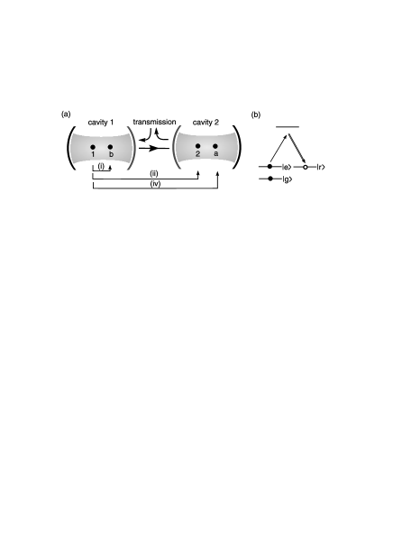
FIG. 1.: (a) Schematic representation of the protocol for ideal transmission of one qubit from atom 1 in cavity 1 to atom 2 in cavity 2. Atom $b$ is a backup atom and $a$ an auxiliary atom. The steps (i)–(v) in the protocol can be found in the text. (b) Level structure of atoms and couplings induced by laser and cavity fields.

We consider the atomic scheme outlined in Fig. 1(b). Three internal long–lived (ground) states levels participate in the transmission. The qubit is stored in $|g\rangle$ and $|e\rangle$, whereas $|r\rangle$ acts as an auxiliary level. To achieve transmision from atom $i$ to $j$, one first transfers $|e\rangle_{i}\rightarrow|r\rangle_{i}$ via a Raman process, where a photon is emitted into a high–Q cavity. The generated photon leaks out of the cavity, propagates along the transmission line, enters the optical cavity at the second node, and induces the inverse transition $|R\rangle_{j}\rightarrow|E\rangle_{j}$ (we will use capital letters to denote the states of the atoms in the second node). In the ideal case, for time $t\rightarrow\infty$ this corresponds to a mapping of the atomic states

$${\cal T}_{i,j}:\begin{array}[]{lll}|g\rangle_{i}|R\rangle_{j}&\rightarrow&|g\rangle_{i}|R\rangle_{j}\\ |e\rangle_{i}|R\rangle_{j}&\rightarrow&|r\rangle_{i}|E\rangle_{j},\end{array}$$ (2)

where the modes of the electromagnetic field are restored to the vacuum.

In reality, there will be errors due to coupling to the environment, as well as systematic errors due to imperfections in adjusting the experimental parameters. We consider the errors that occur during the transmission, and assume that local operations are error-free. The most important errors during transmission will be due to: (1) photon absorption, either in the mirrors or in the transmission line; (2) imperfectly designed laser pulses (including timing, detuning, etc.); the photon wavepacket may be reflected from the second cavity or induce incorrect transfer in the second atom; (3) uncontrolled phase shifts and polarization changes in the transmission line; (4) spontaneous emission during the Raman process. This last error can be strongly suppressed by detuning the laser and the cavity mode from the excited atomic states. Nevertheless, we allow for spontaneous emission to the states $|r\rangle_{i}$ or $|R\rangle_{j}$ [10].

Decoherence and decay may be viewed as a result of a coupling between the system (the two nodes) and the environment. Under the assumption of vanishing correlation time for the reservoir (Markov approximation), the time evolution of the system can be described by a pure state vector evolving according to a nonhermitian effective Hamiltonian ($H_{\rm eff}$) interrupted by quantum jumps at random times. This quantum jump picture of dissipative dynamics underlines the recently developed quantum trajectories methods developed from Monte Carlo integration of quantum optical master equations [11]. More specifically, our present setting [Fig. 1(a)] corresponds to a cascaded quantum system where there is a unidirectional coupling from the first to the second node. The general theory of cascaded quantum systems, in particular the quantum trajectory formulation, was developed by Carmichael and Gardiner [12]. Systematic errors are included in this description as part of the effective Hamiltonian evolution. Within the present model there are two possible evolutions during nonideal transmission, which can be summarized as follows:

(i) With a probability $P$, no jump will occur. The corresponding evolution will be given by

$$\begin{array}[]{l}|g\rangle_{i}|R\rangle_{j}\\ |e\rangle_{i}|R\rangle_{j}\end{array}\stackrel{{\scriptstyle H_{\rm eff}}}{{\longrightarrow}}\begin{array}[]{l}\alpha|g\rangle_{i}|R\rangle_{j}\\ \beta|r\rangle_{i}|E\rangle_{j}+\gamma_{1}|r\rangle_{i}|R\rangle_{j}+\gamma_{2}|e\rangle_{i}|R\rangle_{j}\end{array}$$ (3)

for $t\rightarrow\infty$, where we do not write the state of the cavity modes explicitly since it starts and ends up in the vacuum state $|00\rangle_{c}$. The appearance of population in levels $|r\rangle_{i}|R\rangle_{j}$ and $|e\rangle_{i}|R\rangle_{j}$ may be due to wrongly designed laser pulses. There can also be phase shifts and amplitude damping of the coefficients $\alpha$ and $\beta$, for example, due to photon absorption or spontaneous emission. In general, the complex coefficients $\alpha,\beta$ and $\gamma_{1,2}$ will be functions of (random) external parameters. We will, however, assume for a given complete process (i)–(v) [see Fig. 1(a) and below], $\alpha$ and $\beta$ are the same in the first (ii) and second (iv) transmission [13].

(ii) With a probability $1-P$ a quantum jump will occur corresponding to either photon absorption or spontaneous emission from one of the atoms. The complete process will consist of an evolution according to the effective Hamiltonian, a quantum jump at a random time $\tau$, and followed by the evolution given by $H_{\rm eff}$. For $t\rightarrow\infty$, this can be summarized as

$$\begin{array}[]{l}|g\rangle_{i}|R\rangle_{j}\\ |e\rangle_{i}|R\rangle_{j}\end{array}\stackrel{{\scriptstyle qj}}{{\longrightarrow}}\begin{array}[]{l}0\\ |r\rangle_{i}|R\rangle_{j}\end{array}$$ (4)

where the cavity modes are again restored to the vacuum state. Physically, Eq. (4) can be understood as follows: If a photon is absorbed while propagating from the first to the second cavity, or in the cavity mirrors, this means that it was emitted by atom 1, which ends up in state $|r\rangle_{i}$; atom 2 remains in $|R\rangle_{j}$, since there is no photon to excite it. In a similar way, if the first atom undergoes spontaneous emission to level $|r\rangle_{i}$ during the Raman process, no photon will be transmitted via the channel, and again atom 2 will remain in state $|R\rangle_{j}$. The same reasoning applies to spontaneous emission in atom 2 to level $|R\rangle_{j}$. Note that (4) is a special case of the state mapping (3) with $\alpha=\beta=\gamma_{2}=0$.

We can summarize and formalize the above discussion in the following definition of a noisy channel. Consider the state mapping defined in (3):

• With probability $P\neq 0$, $\alpha,\beta,$ and $\gamma_{1,2}$ are random constants, but $\alpha,\beta$ are the same in two consecutive transmissions [(ii) and (iv) in Fig. 1(a) and see below].

• With probability $1-P$, $\alpha=\beta=\gamma_{2}=0$.

Now we show how to perform ideal transmission over this noisy channel, for arbitrarily small $P$. In the following, normalization factors are left out. We start out with the superposition $(c_{0}|g\rangle_{1}+c_{1}|e\rangle_{1})|g\rangle_{b}|R\rangle_{2}|R\rangle_{a}$. The scheme consists of five steps [Fig. 1(a)]:

(i) Local redundant encoding: Entangle atom 1 with the backup atom $b$ in node 1:

$\displaystyle\left[\!\begin{array}[]{l}|g\rangle_{1}\\ |e\rangle_{1}\end{array}\!\right]\!\otimes\!|g\rangle_{b}|R\rangle_{2}|R\rangle_{a}\rightarrow\left[\!\begin{array}[]{l}|g\rangle_{b}\\ |e\rangle_{b}\end{array}\!\right]\!\otimes\!|\Psi_{i}\rangle+\left[\!\begin{array}[]{l}|e\rangle_{b}\\ |g\rangle_{b}\end{array}\!\right]\!\otimes\!|\Phi_{i}\rangle.$

where

$$|\Psi_{i}\rangle=|e\rangle_{1}|R\rangle_{2}|R\rangle_{b},\quad|\Phi_{i}\rangle=|g\rangle_{1}|R\rangle_{2}|R\rangle_{b}.$$ (5)

In the rest of the scheme atom $b$ will not participate in any process. Thus, we just have to give the evolution of the states $|\Psi_{i}\rangle$ and $|\Phi_{i}\rangle$.

(ii) Transmission from atom 1 to 2: We find

$$|\Psi_{ii}\rangle = \left(\beta|r\rangle_{1}|E\rangle_{2}+\gamma_{1}|r\rangle_{1}|R\rangle_{2}+\gamma_{2}|e\rangle_{1}|R\rangle_{2}\right)\,|R\rangle_{a},$$ (7)

$$|\Phi_{ii}\rangle = \alpha|g\rangle_{1}|R\rangle_{2}|R\rangle_{a}.$$ (8)

Then we measure if atom 1 is left in state $|e\rangle$. If yes, an error has occurred, and the state is collapsed to

$\displaystyle\left[\!\begin{array}[]{l}|g\rangle_{b}\\ |e\rangle_{b}\end{array}\!\right]\!\otimes\!|e\rangle_{1}|R\rangle_{2}|R\rangle_{a}.$

The backup atom is in the pure state $c_{0}|g\rangle_{b}+c_{1}|e\rangle_{b}$, so that we can start again, after resetting the remaining atoms. If atom 1 is not found in state $|e\rangle_{1}$, the corresponding component in (7) is projected out.

(iii) Symmetrization: Perform a local operation on atom 1 that takes $|r\rangle_{1}$ to $|g\rangle_{1}$, and $|g\rangle_{1}$ to $|e\rangle_{1}$, so that

$$|\Psi_{iii}\rangle = \left(\beta|g\rangle_{1}|E\rangle_{2}+\gamma_{1}|g\rangle_{1}|R\rangle_{2}\right)\,|R\rangle_{a},$$ (10)

$$|\Phi_{iii}\rangle = \alpha|e\rangle_{1}|R\rangle_{2}|R\rangle_{a},$$ (11)

By effectively interchanging $|g\rangle_{1}$ and $|e\rangle_{1}$, the unknown coefficients $\alpha$ and $\beta$ of the first transmission are now “symmetrized”: in the next step, $|\Phi\rangle$ will acquire exactly those phase and amplitude errors which $|\Psi\rangle$ acquired in step (ii) [14].

(iv) Transmission from atom 1 to $a$: We obtain

$$|\Psi_{iv}\rangle = \tilde{\alpha}\beta|g\rangle_{1}|E\rangle_{2}|R\rangle_{a}+\tilde{\alpha}\gamma_{1}|g\rangle_{1}|R\rangle_{2}|R\rangle_{a},$$

$$|\Phi_{iv}\rangle = \alpha\tilde{\beta}|r\rangle_{1}|R\rangle_{2}|E\rangle_{a}+\alpha(\tilde{\gamma}_{1}|r\rangle_{1}+\tilde{\gamma}_{2}|e\rangle_{1})|R\rangle_{2}|R\rangle_{a},$$

where the $\tilde{\alpha}$ etc. refer to the second transmission. Then we measure if atom 1 is in $|e\rangle_{1}$. If yes, an error has occurred and the state of atom $b$ can be recovered similar to step (ii). If not, measure if atoms 2 and $a$ are in $|R\rangle_{2}|R\rangle_{a}$. If yes, an error has occurred and we measure the state of atom 1. Depending on the outcome, an appropriate one–bit operation allows us to recover the state from the backup atom. If atoms 2 and $a$ are not found in $|R\rangle_{2}|R\rangle_{a}$, then it implies that no quantum jump has occurred, and therefore, according to our assumption $\alpha=\tilde{\alpha}$ and $\tilde{\beta}=\beta$, the unknown coefficients $\alpha$ and $\beta$ factorize, and thus drop out. The states will be now

$$\left[\!\begin{array}[]{l}|g\rangle_{b}\\ |e\rangle_{b}\end{array}\!\right]\!\otimes\!|g\rangle_{1}|E\rangle_{2}|R\rangle_{a}+\left[\!\begin{array}[]{l}|e\rangle_{b}\\ |g\rangle_{b}\end{array}\!\right]\!\otimes\!|r\rangle_{1}|R\rangle_{2}|E\rangle_{a}.$$ (12)

(v) Teleportation: We measure whether atom $b$ is in $|g\rangle_{b}$ or in $|e\rangle_{b}$. Then we measure if atom 1 is in $|g\rangle_{1}\pm|e\rangle_{1}$. Finally, measure if atom $a$ is in $|E\rangle_{1}\pm|R\rangle_{1}$. Depending on the outcome of these measurements, one can apply an appropriate single atom operation to atom 2 to obtain the original superposition $c_{0}|G\rangle_{2}+c_{1}|E\rangle_{2}$ with probability one. These measurements effectively teleport the state from the first to the second node [15].

We now present numerical simulations of the full problem, to illustrate this error scheme in the context of quantum Monte Carlo wave function simulations for a cascaded quantum system. We take as the effective Hamiltonian for our system (in the rotating frame) [5]

$$H_{{\rm eff}}(t)=\sum_{i=1}^{4}H_{i}(t)-\delta(a_{1}^{\dagger}a_{1}+a_{2}^{\dagger}a_{2})$$ (13)

$$-i\kappa(a_{1}^{\dagger}a_{1}+a_{2}^{\dagger}a_{2}+2a_{2}^{\dagger}a_{1})-i\kappa_{1}^{\prime}a_{1}^{\dagger}a_{1}+\kappa_{2}^{\prime\dagger}a_{2})$$ (14)

where $a_{i}$ is the annihilation operator for a photon in cavity $i=1,2$, $\delta$ is the Raman detuning, $\kappa$ is the decay rate of each cavity, and $\kappa_{1,2}^{\prime}$ are the photon loss rate (in mirrors and transmission channel). This corresponds to the usual one photon damping due to a zero temperature reservoir. A quantum jump amounts to the application of the operators $a_{1,2}$. The Hamiltonian $H_{i}$ for $i=1,2,a,b$ describes the interaction of the atoms with the respective cavity modes and the laser, where the upper level of the $\Lambda$ has been eliminated adiabatically already:

$$H_{i}(t) = \frac{g^{2}}{\Delta+i\Gamma/2}a_{i}^{\dagger}a_{i}|r\rangle_{i}\mbox{}_{i}\langle r|+\delta\omega_{i}(t)|e\rangle_{i}\mbox{}_{i}\langle e|$$ (16)

$$-i\left[g_{i}(t)|e\rangle_{i}\mbox{}_{i}\langle r|-h.c.\right],$$

where $g$ is the coupling constant between atom and cavity mode, $\Delta$ is the laser detuning from the upper state in the $\Lambda$ scheme, $\delta\omega(t)=\frac{1}{4}\Omega(t)^{2}/(\Delta+i\Gamma/2)$ describes both the AC-Stark shift and an effective decay of $|r\rangle$, $g_{i}(t)=\frac{1}{2}g\Omega_{i}(t)/(\Delta+i\Gamma/2)$ is the effective two-photon Rabi frequency (which is complex), in terms of the one-photon Rabi frequency $\Omega_{i}(t)$. In [5] it is described how one constructs the proper laser pulse. The quantum jump corresponding to spontaneous emission amounts to applying the projection operator onto the state $|r\rangle$ [See Fig. 1(b)].

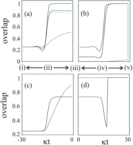
FIG. 2.: Results of Monte–Carlo wave function simulations for the cases of no quantum jump (a,b) and a quantum jump due to photon absorption (c,d). The parameters are: $c_{0}/\sqrt{2}=-0.29+0.25i$, $c_{1}/\sqrt{2}=0.36+0.473i$, $g=5\kappa$, and $\Delta=10\kappa$: (a) Overlap of the state of the system with the ideal state after step (ii) as a function of time for $\Gamma=0$ and $\kappa^{\prime}/\kappa=0,1,10$ (solid, dashed, and dot–dashed line, respectively), and $\Gamma=\kappa^{\prime}=\kappa$ and a 10% error in the Rabi frequencies $\Omega_{1,2}(t)$ (dotted). (b) As in (a) but the overlap with the ideal state after step (iv). (c,d) Overlap with the state $c_{0}|g\rangle_{b}+c_{1}|e\rangle_{b}$ of the back–up atom in the case that a jump occurs during step (iv). Plotted are the cases where $\Gamma=0$, and $\kappa^{\prime}/\kappa=1,10$ (solid and dashed lines, respectively).

Figs. 2a and b illustrate the time evolution of the full system in the case that no jump occurs, and where in the final measurements no error was found (we checked that if an error is found, atom $b$ is in the correct back-up state). Fig. 2a shows the first half of the evolution, where we plot the overlap with the ideal state after step (ii): thus, if there would be no errors, after step (ii) the overlap would be 100%. Fig. 2b shows similarly the overlap with the ideal final state. In the absence of absorption and other errors, both the first and the second gate are indeed found to transfer 100% of the population to the desired (intermediate or final) state. With increasing absorption, there is less and less overlap with the correct state after the first gate, but nevertheless, the second gate completely recovers from this error (for large dissipation this happens only in the final step, in the joint measurement of atoms 2 and $a$), thanks to the ’symmetrization’ of step (iii). We also plot a case where there is spontaneous emission and a 10% error in the laser pulses, and also there the correct final state is reached.

Figs. 2c and d, show a case where a jump occurred in step (iv), where now the overlap of state of the back-up atom with $c_{0}|e\rangle_{b}+c_{1}|g\rangle_{b}$ is displayed. The graph shows that, once the jump occurs, atom 2 will be in that state, and will remain there, also during the remaining operations, so that the initial qubit is fully restored.

Finally, instead of using the language of quantum trajectories, the problem can be formulated by including the environment explicitly. Let us denote by ${\cal T}_{i,j}^{\rm er}$ the unitary transformation for the transmission from atom $i$ to $j$. This corresponds to the state mapping [16]

$$|g\rangle_{i}|R\rangle_{j}|\xi\rangle_{E} \rightarrow |g\rangle_{i}|R\rangle_{j}|\alpha\rangle_{E},$$ (18)

$$|e\rangle_{i}|R\rangle_{j}|\xi\rangle_{E} \rightarrow |r\rangle_{i}|E\rangle_{j}|\beta\rangle_{E}+|r\rangle_{i}|R\rangle_{j}|\gamma_{1}\rangle_{E}$$ (20)

$$+|e\rangle_{i}|R\rangle_{j}|\gamma_{2}\rangle_{E}.$$

where $|\rangle_{E}$ denotes a state of the environment including the cavity modes. In particular, $|\xi\rangle_{E}$ is the initial state, and

$$|\alpha\rangle_{E} = {}_{i}\!\langle g|\;{}_{j}\!\langle R|{\cal T}_{i,j}^{\rm er}|g\rangle_{i}|R\rangle_{j}|\xi\rangle_{E}\equiv T|\xi\rangle_{E},$$ (22)

$$|\beta\rangle_{E} = {}_{i}\!\langle r|\;{}_{j}\!\langle E|{\cal T}_{i,j}^{\rm er}|e\rangle_{i}|R\rangle_{j}|\xi\rangle_{E}\equiv S|\xi\rangle_{E},$$ (23)

and analogously for the other states of the environment. Ideal transmission can be accomplished again following steps (i)–(v). The condition that $\alpha$ and $\beta$ remain the same in the steps (ii) and (iv) is replaced by $ST|\xi\rangle_{E}=TS|\xi\rangle_{E}$. This is fulfilled, for example, when the Markov approximation applies: this means that we effectively couple to independent reservoirs in the first (ii) and second (iv) transmission.

In conclusion, we have presented a scheme which achieves perfect transmission in a “noisy” quantum network via photon exchange. The protocol corrects the dominant errors that occur in a physically realistic situation. The distinguishing feature of our scheme is that one can repeat the transmission operation as many times as needed to accomplish ideal transfer. We believe that this is a fundamental theoretical result towards implementing experimentally quantum communication networks.

We thank D. DiVincenzo, H.J. Kimble, and H. Mabuchi for discussions. This work was supported in part by the TMR network ERB–FMRX–CT96–0087, and by the Austrian Science Foundation.

REFERENCES

- [1] C. H. Bennett, Phys. Today, Vol. 24 (October 1995).
- [2] B. Schumacher, Phys. Rev. A 45, 2614 (1996).
- [3] C.H. Bennett et al, Phys. Rev. Lett. 76, 722 (1996); A. Ekert and C. Macchiavello, ibid, 77, 2585 (1996).
- [4] See also C.H. Bennett and S.J. Wiesner, Phys. Rev. Lett. 69, 2881 (1992); K. Mattle et al., ibid. 76, 4656 (1996).
- [5] J.I. Cirac et al., quant-ph/9611017.
- [6] P.W. Shor, Phys. Rev. A 52, 2493 (1995). A.M. Steane, Phys. Rev. Lett. 77, 793 (1996); E. Knill and R. Laflamme, Phys. Rev. A (in press); J.I. Cirac, T. Pellizzari, and P. Zoller, Science 273, 1207 (1996).
- [7] To achieve first-order error correction, five physical qubits are required. R. Laflamme et al., Phys. Rev. Lett. 77, 3240 (1996)
- [8] Q. Turchette et al., Phys. Rev. Lett. 75, 4710 (1995).
- [9] J.I. Cirac and P. Zoller, Phys. Rev. lett. 74, 4091 (1995); C. Monroe et al., Phys. Rev. Lett. 75, 4714 (1995).
- [10] We do not allow for spontaneous emission back to the state or . This could be suppressed, for example, by driving a forbidden transition with the laser, or by tuning the laser between two excited atomic states to cancel spontaneous emission by destructive interference, by N. Lütkenhaus et al., unpublished.
- [11] P. Zoller and C.W. Gardiner, in Quantum Fluctuations, Les Houches, eds. E. Giacobino et al., Elsevier, in press.
- [12] C.W. Gardiner, Phys. Rev. Lett. 70, 2269 (1993); H.J. Carmichael, ibid. 70, 2273 (1993);
- [13] This means, for example, that we synthesize a laser pulse, duplicate and time delay it, and use the identical but imperfect pulses in the first and second transmission.
- [14] T. Pellizzari et al., Phys. Rev. Lett. 75, 3788 (1995).
- [15] In our protocol, ideal transmission is achieved eventhough our noisy channel has a zero probability for no error (i.e. ). The capacity of noisy channels with finite probability of no errors has recently been studied C.H. Bennett, D.P. DiVincenzo and J.A. Smolin, quant-ph/9701015.
- [16] This transformation can be generalized to include additional atomic states, which will require additional measurements.