Quantum Noise in Quantum Optics:
the Stochastic Schrödinger Equation

Abstract

Lecture Notes for the Les Houches Summer School LXIII on Quantum Fluctuations in July 1995: “Quantum Noise in Quantum Optics: the Stochastic Schroedinger Equation” to appear in Elsevier Science Publishers B.V. 1997, edited by E. Giacobino and S. Reynaud.

0.1 Introduction

Theoretical quantum optics studies “open systems,” i.e. systems coupled to an “environment” [2, 3, 4, 5]. In quantum optics this environment corresponds to the infinitely many modes of the electromagnetic field. The starting point of a description of quantum noise is a modeling in terms of quantum Markov processes [2]. From a physical point of view, a quantum Markovian description is an approximation where the environment is modeled as a heatbath with a short correlation time and weakly coupled to the system. In the system dynamics the coupling to a bath will introduce damping and fluctuations. The radiative modes of the heatbath also serve as input channels through which the system is driven, and as output channels which allow the continuous observation of the radiated fields. Examples of quantum optical systems are resonance fluorescence, where a radiatively damped atom is driven by laser light (input) and the properties of the emitted fluorescence light (output)are measured, and an optical cavity mode coupled to the outside radiation modes by a partially transmitting mirror.

Historically, the first formulations were given in terms of quantum Langevin equations (as developed in the context of laser theory) which are Heisenberg equations for system operators with the reservoir eliminated in favor of damping terms and white noise operator forces (see references in [2]). The alternative and equivalent formulation in terms of a master equation for a reduced system density operator together with the quantum fluctuation regression theorem, has provided the most important practical tool in quantum optics, in particular for nonlinear systems [2, 3].

The rigorous mathematical basis for these methods is quantum stochastic calculus (QSC) as formulated by Hudson and Parthasarathy [6]. QSC is a noncommutative analogue of Ito’s stochastic calculus [7]. The basic ingredients are “white noise” Bose fields $b(t)$, $b(t)^{\dagger}$ with canonical commutation relations $[b(t),b(t^{\prime})^{\dagger}]=\delta(t-t^{\prime})$. In quantum optics these Bose fields can be considered as an approximation to the electromagnetic field. The connection between these abstract mathematical developments and the physical principles and foundations of quantum optics is discussed in particular in the work of Barchielli [8, 9, 10, 11, 12], and Gardiner and coworkers [2, 13, 14]. Gardiner and Collett [13] showed the connection between the more physically motivated quantum Langevin equations and the more mathematically precise “quantum stochastic differential equations” (QSDE). Furthermore, these authors introduced as an essential element of the theory an interpretation of the Bose–fields as “input” and “output” fields corresponding to the field before and after the interaction with the system. QSC allows also the development of a consistent theory of photodetection (photon counting and heterodyne measurements) [12, 15] in direct relationship with the theory of continuous measurement of Srinivas and Davies [16].

While most of the theoretical work in quantum optics has emphasized quantum Langevin and master equations [2], recent developments and applications have focused on formulations employing the quantum stochastic Schrödinger equation (QSSE) [10, 11, 14, 17] and its c-number version, a stochastic Schrödinger equation (SSE) [3, 11, 12, 14, 15, 17, 18, 19, 20, 21, 22, 23, 24, 25, 26, 27, 28, 29, 30, 31, 32, 33, 34]. Phenomenological SSEs have been given in Refs. [35, 36, 37, 38]. The QSSE is a QSDE for the state vector of the combined system + heatbath with Bose fields $b(t)$ and $b(t)^{\dagger}$ as noise operators. This equation generates a unitary time evolution, and implies the master equation and the quantum regression theorem for multitime averages, and the Quantum Langevin equation for system operators as exact results.

The SSE, on the other hand, is a stochastic evolution equation for the system wave function with damping and c–number noise terms which implies a non-unitary time evolution. The relationship between the QSSE and the SSE is established by the continuous measurement formalism of Srinivas and Davies for counting processes (photon counting)[16]. This continuous measurement theory has the interpretation as a probabilistic description in terms of quantum jumps in a system. Thus the continuous measurement theory can be simulated probabilistically, and this simulation yields a sequence of system wave functions with jumps at times $t_{1},t_{2},\ldots,t_{n}$ by a rule which is directly related to the structure of the appropriate QSDE. The trajectories of counts generated in these simulations have the same statistics as the photon statistics derived within the standard photodetection theory, and in this sense the individual counting sequences generated in a single computer run can, with some caution, be interpreted as “what an observation would yield in a single run of the experiment.” These simulations can thus illustrate the dynamics of single quantum systems, for example in the quantum jumps in ion traps [39] or the squeezing dynamics [3]. In continuous measurement theory the time evolution of the system conditional on having observed (or simulated) a certain count sequence is called a posteriori dynamics. The master equation is recovered in this description as ensemble average over all counting trajectories. Again, in the language of continuous measurement theory, this corresponds to a situation where the measurements (the counts) are not read, i.e. no selection is made (a priori dynamics). Simulation of the SSE and averaging over the noise provides an new computational tool to generate solutions of the master equation. An important feature, first emphasized by Dalibard, Castin and Mølmer [18] is that one only has to deal with a wave function of dimension $N$, as opposed to working with the density matrix which has $N^{2}$ elements. Thus, simulations can provide solutions when a direct solution of the master equation is impractical because of the large dimension of the system space.

When instead of direct photon counting we perform a homodyne experiment, where the system output is mixed with a local oscillator, and a homodyne current is measured, the jumps are replaced by a diffusive evolution. These diffusive Schrödinger equations were first derived by Carmichael [3, 15] from his analysis of homodyne detection, and independently in a more formal context by Barchielli and Belavkin [12]. Somewhat earlier equations of this form have been postulated in connection with dynamical theories of wave function reduction [35, 36, 38].

In these notes we will review in a pedagogical way some of the recent developments of quantum noise methods, continuous measurement and the stochastic Schrödinger equation and some applications, and the main purpose is to emphasize and illustrate the physical basis of such a formulation.

0.2 An introductory example: Mollow’s pure state analysis of resonant light scattering

As an introduction and historical remark we briefly review Mollow’s work on the pure state analysis of resonant light scattering [40]. Twenty years ago Mollow developed a theory of resonance fluorescence of a strongly driven two–level atom, where he showed that the atomic density matrix could be decomposed into contributions from subensembles corresponding to a certain trajectory of photon emissions, which could be represented by atomic wave functions. This formulation anticipated and provided the basis [14, 20, 39] for some of the recent developments in quantum optics from the Stochastic Schrödinger Equation for system wave functions to our understanding of the photon statistics in the framework of continuous measurement theory. Below we will briefly review some of Mollow’s ideas in a more modern language, closely related to the discussions of the following sections.

Hierarchy of equations

We consider a two–level system with ground state $|g\rangle$ and excited state $|e\rangle$ which is driven by a classical light field and coupled to a heatbath of radiation modes. The starting point of the derivation of Mollow’s pure state analysis is the definition of a reduced atomic density operator in the subspace containing exactly $n$ scattered photons according to

$$\rho^{(n)}(t)={\rm Tr}_{B}\{{\hat{P}}^{(n)}{\hat{\rho}}(t)\}\quad\mbox{($n=0,1,2,\ldots$)}$$ (1)

with ${\hat{\rho}}(t)$ the density operator of the combined atom + field system, ${\hat{P}}^{(n)}$ the projection operator onto the $n$-photon subspace, and ${\rm Tr}_{B}$ indicating the trace over the radiation modes. The probability of finding exactly $n$ photons in the field is

$$P^{(n)}(t)={\rm Tr}_{S}\rho^{(n)}(t)\equiv\rho^{(n)}_{gg}(t)+\rho^{(n)}_{ee}(t)$$ (2)

with ${\rm Tr}_{S}$ the trace over the atomic variables (the “system”). It has been pointed out in Refs. [40, 41, 39] that $\rho^{(n)}(t)$ obeys the equation of motion

$$\frac{d}{dt}\rho^{(n)}(t)=-i\left(H_{\rm eff}\rho^{(n)}(t)-\rho^{(n)}(t)H_{\rm eff}^{\dagger}\right)+\Gamma\sigma_{-}\rho^{(n-1)}(t)\sigma_{+}\;.$$ (3)

Here

$$H_{\rm eff}=(-\Delta-i\frac{1}{2}\Gamma)\sigma_{ee}-\left(\frac{1}{2}\Omega\sigma_{+}+H.c.\right)$$ (4)

is the non–hermitian Wigner-Weisskopf Hamiltonian of the radiatively damped and driven two–level atom with $\sigma_{+}=|e\rangle\langle g|$, $\sigma_{-}=|g\rangle\langle e|$, $\sigma_{z}=|e\rangle\langle e|-|g\rangle\langle g|=\sigma_{ee}-\sigma_{gg}$ the Pauli spin matrices describing a two–level atom, $\Delta$ the laser detuning, $\Gamma$ the spontaneous decay rate of the upper state of the two-level system and $\Omega$ the Rabi frequency. Summing over the $n$–photon contributions

$$\rho(t)=\sum_{n=0}^{\infty}\rho^{(n)}(t)$$ (5)

with $\rho(t)$ the reduced atomic density operator, Eq. (3) reduces to the familiar optical Bloch equations (OBEs)

$$\frac{d}{dt}\rho(t)=-i\left(H_{\rm eff}\rho(t)-\rho(t)H_{\rm eff}^{\dagger}\right)+\Gamma\sigma_{-}\rho(t)\sigma_{+}\;.$$ (6)

The $n$–photon density matrix $\rho^{(n)}(t)$ is seen to obey a hierarchy of equations where the $n-1$ photon density matrix provides the feeding term for the $n$–photon term, $\ldots\rightarrow\rho^{(n-1)}\rightarrow\rho^{(n)}\ldots$. By formal integration of this hierarchy we obtain Mollow’s pure state representation of the atomic density matrix

$$\rho(t)=|{\tilde{\psi}}_{c}(t)\rangle\langle{\tilde{\psi}}_{c}(t)| +\sum_{n=1}^{\infty}\int_{0}^{t}dt_{n}\int_{0}^{t_{n}}dt_{n-1}\ldots\int_{0}^{t_{2}}dt_{1}$$ (8)

$$|{\tilde{\psi}}_{c}(t|t_{n},t_{n-1},\ldots,t_{1})\rangle\langle{\tilde{\psi}}_{c}(t|t_{n},t_{n-1},\ldots,t_{1})|$$

with atomic wave functions obeying the equation of motion

$$\frac{d}{dt}|{\tilde{\psi}}_{c}(t|t_{n},\ldots,t_{1})\rangle=-iH_{\rm eff}|{\tilde{\psi}}_{c}(t|t_{n},\ldots,t_{1})\rangle\quad\mbox{($t\geq t_{n}\geq t_{n-1}\geq\dots\geq t_{1}$)}$$ (9)

and defined recursively by the jump condition

$$|{\tilde{\psi}}_{c}(t_{n}|t_{n},t_{n-1},\ldots,t_{1})\rangle=\sqrt{\Gamma}\sigma_{-}|{\tilde{\psi}}_{c}(t_{n}|t_{n-1},\ldots,t_{1})\rangle$$ (10)

with $|\!|{\tilde{\psi}}_{c}(t=0)|\!|=1$. Eq. (8) gives the atomic density matrix in terms of pure atomic states ${\tilde{\psi}}_{c}(t|t_{n},\ldots,t_{1})$.

Interpretation

The essential features behind this construction are as follows. According to Mollow [40] Eq. ( 8) can be interpreted as the time evolution of an atom in a time interval $(0,t]$ which emits exactly $n$ photons at times $t_{1},t_{2},\ldots,t_{n}$. According to (10) atoms in the ground state with $n$ photons in the scattered field are created at a rate $\Gamma|\!|\sigma_{-}{\tilde{\psi}}_{c}(t|t_{n-1},\ldots,t_{1})|\!|^{2}$. Each photon emission is accompanied by a reduction of the atomic wave function to the ground state $|g\rangle$ as described by the operator $\sigma_{-}$ in Eq. (10). This is what we call a quantum jump. The time evolution between the photon emissions is governed by the non–hermitian Wigner–Weisskopf Hamiltonian $H_{\rm eff}$ which describes the reexcitation of the radiatively damped atom by the laser field.

As has been pointed out in Ref. [39] in the context of discussion of quantum jumps in three-level systems [41, 42], Eq. (8) has the structure expected from the Srinivas Davies theory of continuous measurement for counting processes [16], and in particular supports the interpretation of

$$p_{0}^{t}(t_{n},\ldots,t_{1})=|\!|{\tilde{\psi}}_{c}(t|t_{n},\ldots,t_{1})|\!|^{2}$$ (11)

as an exclusive probability density that the atom emits $n$ photons a times $t_{1},t_{2},\ldots,t_{n}$ (and no other photons) in the time interval $(0,t]$. Thus the time evolution can be simulated: Fig. 1 shows the excited state population $|\langle e|\psi_{c}(t)\rangle|^{2}$ with normalized wavefunction $\psi_{c}(t)={\tilde{\psi}}_{c}(t)/|\!|{\tilde{\psi}}_{c}(t)|\!|$, corresponding to a single run as a function of time for a Rabi frequency $\Omega=\Gamma$ and detuning $\Delta=-\Gamma$. The decay times (indicated by arrows) and quantum jumps where the atomic electron returns to the ground state are clearly visible as interruptions of the Rabi oscillations. After a quantum jump the atom reset is to the ground state, and it then is reexcited by the laser: in the photon statistics of the emitted light this leads to antibunching, i.e. two photons will not be emitted at the same time [4]. Averaging over these trajectories gives the familiar transient solution of the optical Bloch equation. Although Mollow’s derivation and somewhat intuitive interpretation was restricted to a specific example, the basic structure and ideas which emerge from his analysis are valid in a much more general context which is what we will be concerned with in the following sections.

Figure 1: Plot of a realization of the Monte Carlo wavefunction as a function of time: excited state probability $|\langle e|\psi_{c}(t)\rangle|^{2}$ [20].

0.3 Wave-function quantum stochastic differential equations

0.3.1 The Model

The standard model of quantum optics [2, 11] considers a system interacting with a heatbath consisting of many harmonic oscillators representing the electromagnetic field. The Hamiltonian for the combined system is ($\hbar=1$)

$$H_{\rm tot}=H_{\rm sys}+H_{\rm B}+H_{\rm int}$$ (12)

with

$$H_{\rm B}=\int\,d\omega\,\omega\,b(\omega)^{\dagger}b(\omega)$$ (13)

the Hamiltonian for the heatbath, and $b(\omega)$ the annihilation operator satisfying the canonical commutation relations (CCR)

$$[b(\omega),b(\omega)^{\dagger}]=\delta(\omega-\omega^{\prime})\;.$$ (14)

For simplicity, we assume only a single heatbath. Generalization to many reservoirs represents no conceptual difficulty. The interaction Hamiltonian (15) is based on a linear system – field coupling in a rotating wave approximation (RWA),

$$H_{\rm int}=i\frac{1}{\sqrt{2\pi}}\int\,d\omega\,\kappa(\omega)[cb(\omega)^{\dagger}-b(\omega)c^{\dagger}]$$ (15)

with $c$ a system operator (the “system dipole”), and $\kappa(\omega)$ coupling functions. The system Hamiltonian $H_{\rm sys}$ is left unspecified.

Approximations

Quantum noise theory is based on the following approximations [2]: (i) Rotating wave approximation (RWA) and smooth system–bath coupling, and (ii) a Markov (white noise) approximation.

• Rotating wave approximation: For simplicity, we assume that for the bare (interaction free) system the system dipole $c$ evolves as $c(t)=ce^{-i\omega_{0}t}$ with $\omega_{0}$ the resonance frequency of the system. Thus the system will be dominantly coupled to a band of frequencies centered around $\omega_{0}$. Validity of the RWA requires that the frequency integration in $H_{\rm int}$ is restricted to a range of frequencies

  $$\int_{\omega_{0}-\vartheta}^{\omega_{0}+\vartheta}\,d\omega\ldots\,$$ (16)

  with cutoff $\vartheta\ll\omega_{0}$. This assumes a separation of time scales: the optical frequency $\omega_{0}$ is much larger than the cutoff $\vartheta$ which again is much larger than the typical frequencies of the system dynamics and frequency scale induced by the system – bath couplings (decay rates). Furthermore, we assume a smooth system–bath coupling $\kappa(\omega)$ in the frequency interval (16): we set $\kappa(\omega)\rightarrow 1$ (a constant factor can always be reabsorbed in a definition of $c$).

  We transform to the interaction picture with respect to the free dynamics of the “bare system + field.” In the interaction Hamiltonian (15) this amounts to the replacements $c\rightarrow ce^{-i\omega_{0}t}$, $b(\omega)\rightarrow b(\omega)e^{-i\omega t}$, so that in the interaction picture the interaction Hamiltonian becomes

  $$H_{\rm int}^{(\vartheta)}(t)=i[b^{(\vartheta)}(t)^{\dagger}c-b^{(\vartheta)}(t)c^{\dagger}]$$ (17)

  with

  $$b^{(\vartheta)}(t)=\frac{1}{\sqrt{2\pi}}\int_{\omega_{0}-\vartheta}^{\omega_{0}+\vartheta}\,d\omega\;b(\omega)e^{-i(\omega-\omega_{0})t}\,.$$ (18)

  The time evolution operator $U^{(\vartheta)}(t)$ from time $0$ to $t$ in the interaction picture obeys the Schrödinger equation

  $$\frac{d}{dt}U^{(\vartheta)}(t)=-i(H+H_{\rm int}^{(\vartheta)}(t))U^{(\vartheta)}(t)$$ (19)

  with $H$ the transformed system Hamiltonian. Note that by going to the interaction picture “fast” optical frequencies $\omega_{0}$ have disappeared (“transformation to a rotating frame”).

• The Markov approximation or white noise approximation: this consists of taking the limit $\vartheta\rightarrow\infty$ in Eq. (19),

  $$b^{(\vartheta)}(t)\rightarrow b(t):=\frac{1}{\sqrt{2\pi}}\int_{-\infty}^{\infty}\,d\omega b(\omega)e^{-i(\omega-\omega_{0})t}\,.$$ (20)

  so that the commutator for the fields $b(t)$ in the time domain acquires a $\delta$–function form,

  $$[b(t),b(t^{\prime})^{\dagger}]=\delta(t-t^{\prime})\;.$$ (21)

  The operator $b(t)$ is a driving field for the equation of motion (19) at time $t$. In the following we should interpret the parameter $t$ to mean the time at which the initial incoming field will interact with the system, rather then specifying that $b(t)$ is a time-dependent operator at time $t$.

0.3.2 Quantum Stochastic Calculus

The commutator (21) is a $\delta$–function because of the Markov approximation. The Markovian equations that result have a greatly simplified form, but this simplification arises at the expense of having to define stochastic calculus, leading to the concepts of Ito and Stratonovich integration much as in the classical case. We give here a heuristic review of these ideas.

Quantum stochastic calculus (QSC) is a non-commutative analogue of Ito’s stochastic calculus. It was developed originally as a mathematical theory of quantum noise in open system and more recently found application to measurement theory in quantum mechanics.

For simplicity we consider the situation in which the field is in a vacuum state, so that $b(t)|\rm vac\rangle=0$, and thus $\left\langle b(t)b^{\dagger}(t^{\prime})\right\rangle=\langle\mbox{\rm vac}|b(t)b^{\dagger}(t^{\prime})|\mbox{\rm vac}\rangle=\delta(t-t^{\prime})$ and $\left\langle b^{\dagger}(t)b(t^{\prime})\right\rangle=0$. We define

$$B(t):=\int_{0}^{t}\,ds\,b(s),\quad B(t)^{\dagger}:=\int_{0}^{t}\,ds\,b(s)^{\dagger}\;.$$ (22)

For the vacuum averages these definitions lead to

$$\left\langle[B(t)-B(t_{0})][B(t)^{\dagger}-B(t_{0})^{\dagger}]\right\rangle=|t-t_{0}|\\$$ (23)

$$\left\langle B(t)-B(t_{0})\right\rangle=\left\langle[B(t)^{\dagger}-B(t_{0})^{\dagger}]^{2}\right\rangle=\left\langle[B(t)-B(t_{0})]^{2}\right\rangle=0\,.$$ (24)

A quantum stochastic calculus of the Ito type, based on the increments

$$dB(t)=B(t\!+\!dt)-B(t),\quad dB(t)^{\dagger}=B(t\!+\!dt)^{\dagger}-B(t)^{\dagger}$$ (25)

and $dt$ has been developed by Hudson and Parthasarathy [6]. The pair $B(t)$, $B(t)^{\dagger}$ are the non–commutative analogues of complex classical Wiener processes.

Quantum stochastic integration

We consider two definitions of quantum stochastic integration: Ito,

$$\int_{0}^{t}\,f(s)\,dB(s)=\lim_{n\rightarrow\infty}\sum_{i=0}^{n}f(t_{i})[B(t_{i+1})-B(t_{i})]$$ (26)

and Stratonovich

$$\mbox{ \bf(S)}\int_{0}^{t}\,f(s)\,dB(s)=\lim_{n\rightarrow\infty}\sum_{i=0}^{n}\frac{1}{2}[f(t_{i+1})+f(t_{i})][B(t_{i+1})-B(t_{i})]\,.$$ (27)

In both cases $f(t)$ is a nonanticipating (or adapted) function, i.e. an operator valued quantity which depends only on $B(s)$ etc. for $s<t$. There are analogous definitions for the Ito and Stratonovich versions of

$$\int_{0}^{t}\,f(s)\,dB(s)^{\dagger},\int_{0}^{t}\,dB(s)\,f(s),\int_{0}^{t}\,dB(s)^{\dagger}\,f(s).$$ (28)

The basic difference between the Ito and Stratonovich form of the integrals is that in the Ito form the term $f(t_{i})$ and $[B(t_{i+1})-B(t_{i})]$ are independent of each other, whereas in the Stratonovich form $[f(t_{i+1})+f(t_{i})]$ is not independent of $[B(t_{i+1})-B(t_{i})]$.

Example and discussion

If we use the property (23), we find

$$\left\langle\int_{0}^{t}\,dB(s)B(s)^{\dagger}\right\rangle=0$$ (29)

$$\left\langle\mbox{ \bf(S)}\int_{0}^{t}\,dB(s)B(s)^{\dagger}\right\rangle=\frac{1}{2}|t|\,.$$ (30)

In fact this example shows the three main principles involved.

1. Stratonovich integration follows the rules of conventional calculus. For example, the conventional differential of $B(t)B(t)^{\dagger}$ is the Stratonovich differential

   $$({\rm S})\,d(B(t)B(t)^{\dagger})=\,dB(t)B(t)^{\dagger}+B(t)\,dB(t)^{\dagger}$$ (31)

   so that

   $$\left.B(t)B(t)^{\dagger}\right|_{0}^{t}=\mbox{ \bf(S)}\int\limits_{0}^{t}\,dB(s)B(s)^{\dagger}+\mbox{ \bf(S)}\int_{0}^{t}B(s)\,dB(s)^{\dagger}$$ (32)

   and using (23,27) and taking averages, we find

   $$|t|={1\over 2}|t|+{1\over 2}|t|$$ (33)

   as should be the case.

2. Ito Integration increments are independent of and commute with the integrand. From this independence we see that we can factorize the average so that

   $$\left\langle\int_{0}^{t}\,\,dB(s)\,B(s)^{\dagger}\right\rangle=\int\left\langle dB(s)\right\rangle\left\langle B(s)^{\dagger}\right\rangle=\int_{0}^{t}\,0=0$$ (34)

   For Ito differentials the conventional rule (31) is replaced by the rules:

   1. Expand all differentials to second order.

   2. Use the multiplication rules [for a vacuum state—otherwise use the rules (62)]

      $$dt^{2}=dB^{2}(t)=dB(t)^{{\dagger}^{2}} = \,dB^{\dagger}(t)\,dB(t)=0$$

      $$\,dB(t)dt=\,dB(t)^{\dagger}\,dt = dt\,\,dB(t)=dt\,\,dB(t)^{\dagger}=0$$

      $$dB(t)\,dB(t)^{\dagger} = dt\,.$$ (35)

   Using these rules, we find

   $$d\left[B(t)B^{\dagger}(t)\right] = dB(t)B(t)^{\dagger}+B(t)\,dB(t)^{\dagger}+\,dB(t)\,dB(t)^{\dagger}$$ (36)

   $$= dB(t)\,B(t)^{\dagger}+B(t)\,dB(t)^{\dagger}+dt\,,$$

   so that using the Ito integral, we get

   $$\left\langle B(t)B(t)^{\dagger}\right\rangle|_{0}^{t}=|t|=0+0+|t|\,$$ (37)

   in agreement with (33). These rules are sufficient for ordinary manipulation, but are defined only when the state is the vacuum. Rules for non-vacuum states will be discussed briefly at the end of this section.

3. The mean value of an Ito integral is always zero. This follows from the independence of $\,dB(t)=B(t\!+\!dt)-B(t)$ and $f(t)$, which has been assumed to be nonanticipating.

As in the case of classical stochastic differential equations, an equation

$$\frac{d}{dt}X(t)=F(X(t),t)+G(X(t),t)\,b(t)+H(X(t),t)\,b^{\dagger}(t)$$ (38)

cannot be rigorously considered as a differential equation, since the terms involving $b(t)$ and $b^{\dagger}(t)$ are in some sense infinite. However this equation can be regarded as an integral equation

$$X(t)-X(t_{0})=\int_{t_{0}}^{t}dX(t^{\prime})$$

$$=\int_{t_{0}}^{t}\left\{F(X(t^{\prime}),t^{\prime})\,dt^{\prime}+G(X(t^{\prime}),t^{\prime})\,dB(t^{\prime})+H(X(t^{\prime}),t^{\prime})\,dB^{\dagger}(t^{\prime})\right\}$$

As in the case of non-quantum stochastic differential equations, a simplified notation is used, in which the explicit symbols of integration are dropped:

$$dX(t) = F(X(t),t)\,dt+G(X(t),t)\,dB(t)+H(X(t),t)\,dB(t)^{\dagger}$$ (40)

which is known as a stochastic differential equation.

Comparison of Ito and Stratonovich Stochastic Differential Equations (SDE)

The Stratonovich definition is natural for physical situations where the white noise approximation is an idealization. While the Stratonovich form has its merits of satisfying ordinary calculus, the equation as it stands is rather like an implicit algorithm for the solution of a differential equation which makes manipulations rather difficult.

In the Ito definition the differentials $dB(t)=B(t\!+\!dt)-B(t)$ etc. point to the future. Quantum stochastic Ito calculus obeys simple formal rules which can be summarized as follows:

1. By the CCR (14) nonanticipating functions $X(t)$ commute with the fundamental differentials, $[X(t),dB(t)]=0$ etc..

2. For two functions $X(t)$ and $Y(t)$ satisfying equations of the type (40), the differential of the product $X(t)Y(t)$ is given by

   $$d[X(t)Y(t)]=[dX(t)]\,Y(t)+X(t)\,[dY(t)]+dX(t)\,dY(t)$$ (41)

   where the Ito correction (the last term on the RHS of Eq.(41)) has to be computed by means of the Ito table

   $$dB(t)\,dB(t)^{\dagger}=dt\quad\mbox{(vacuum state)}$$ (42)

   and all other products involving $dB(t)$, $dB(t)^{\dagger}$ and $dt$ vanish.

0.3.3 Quantum Stochastic Schrödinger, Density Matrix and Heisenberg Equations

The definition of Ito and Stratonovich integration allows us to give meaning to a quantum stochastic Schrödinger equation for the time evolution operator ${\hat{U}}(t)$ of the system interacting with Bose fields $b(t)$, $b^{\dagger}(t)$. The Schrödinger equation (19) must be interpreted as a Stratonovich SDE

$$\mbox{ \bf(S)}\,d{\hat{U}}(t)=\{-iH\,dt+dB(t)^{\dagger}c-dB(t)c^{\dagger}\}{\hat{U}}(t)\,.$$ (43)

It is advantageous to convert this Stratonovich equation to Ito form. By conversion to Ito form, we can get a modified equation in which the increments $dB(t)$, $dB(t)^{\dagger}$ and independent of ${\hat{U}}(t)$. This Ito form of the quantum stochastic Schrödinger equation is

$$\,d{\hat{U}}(t)=\{(-iH-\frac{1}{2}c^{\dagger}c)\,dt+dB(t)^{\dagger}\,c-dB(t)\,c^{\dagger}\}{\hat{U}}(t)\quad({\hat{U}}(0)=\hat{1}).$$ (44)

As the solution ${\hat{U}}(t)$ of (44) is nonanticipating, since the increments $dB(t)$, $dB(t)^{\dagger}$ point to the future, we have $[{\hat{U}}(t),dB(t)]=[{\hat{U}}(t),dB(t)^{\dagger}]=0$.

Remark: Conversion from Stratonovich to Ito form: this conversion proceeds analogous to the classical case. Consider the Ito equation

$$\,d{{\hat{U}}(t)}=\left\{\alpha\,dt+\beta dB(t)^{\dagger}-\beta^{\dagger}dB(t)^{\dagger}\right\}{{\hat{U}}(t)}$$ (45)

We consider an arbitrary Stratonovich integral of a function $|\phi(t)\rangle={\hat{U}}(t)|\phi(0)\rangle$ which obeys Eq. (45)

$$\mbox{ \bf(S)}\int\,dB(t){\phi(t)} = \lim\sum\Delta B_{i}\frac{1}{2}[{\phi(t_{i+1})}+{\phi(t_{i})}]$$

$$= \lim\sum\Delta B_{i}[{\phi(t_{i})}+\frac{1}{2}(\alpha\Delta t_{i}+\beta\Delta B_{i}^{\dagger}-\beta^{\dagger}\Delta B_{i}){\phi(t_{i})}]$$

and by $\Delta B_{i}\,\Delta B_{i}^{\dagger}\rightarrow\Delta t_{i}$

$$\mbox{ \bf(S)}\int\,dB(t){\phi(t)} = \lim\sum\left\{\Delta B_{i}{\phi(t_{i})}+\frac{1}{2}\beta\Delta t_{i}{\phi(t_{i})}\right\}$$

$$= \int\,dB(t)\,{\phi(t)}+\frac{1}{2}\int\,dt\,\beta\,{\phi(t)}$$

and similar expressions for the other integrals. Remembering that (45) is a shorthand for an integral equation we see that (45) is equivalent to (43) if $\beta=c$, $\beta^{\dagger}=c^{\dagger}$, $\alpha=-iH-\frac{1}{2}c^{\dagger}c$.

The formal solution of the Eq. (44) can be written as

$${\hat{U}}(t)=T\,{\rm exp}{\int_{0}^{t}\,\left(-iH\,ds+dB(s)^{\dagger}c-dB(s)\,c^{\dagger}\right)}$$ (48)

where $T$ denotes the time–ordered product. This equation gives

$$d{\hat{U}}(t) \equiv {\hat{U}}(t\!+\!dt)-{\hat{U}}(t)=\left[{\rm exp}{\left(-iH\,dt+dB(t)^{\dagger}c-dB(t)\,c^{\dagger}\right)}-1\right]{\hat{U}}(t)$$ (49)

$$= \sum_{n=1}^{\infty}\frac{1}{n!}\left(-iH\,dt+dB(t)^{\dagger}c-dB(t)\,c^{\dagger}\right)^{n}{\hat{U}}(t)\;.$$

Applying the Ito rules (42), terms with $n>2$ vanish, the term with $n=1$ gives $-iH\,dt+dB(t)^{\dagger}c-dB(t)\,c^{\dagger}$, $n=2$ gives $-\frac{1}{2}c^{\dagger}c\,dt$, and we recover Eq. ( 44). Obviously, from Eq. (48) ${\hat{U}}(t)$ is unitary.

The state vector $|\Psi(t)\rangle={\hat{U}}(t)|\Psi(0)\rangle$ with initial condition $|\Psi(0)\rangle=|\psi\rangle\otimes|\rm vac\rangle$ obeys a stochastic Schrödinger equation

$$\,d|\Psi(t)\rangle=\{(-iH-\frac{1}{2}c^{\dagger}c)\,dt+dB(t)^{\dagger}\,c-dB(t)\,c^{\dagger}\}|\Psi(t)\rangle\,.$$ (50)

Since $|\Psi(0)\rangle$ contains the vacuum of the electromagnetic field, $b(\omega)|\Psi(0)\rangle=0$ and thus $dB(t)|\Psi(0)\rangle=0$. Because ${\hat{U}}(t)$ commutes with $dB(t)$ it follows that $dB(t)|\Psi(t)\rangle=0$. This means, as far as $dB(t)$ is concerned, $|\Psi(t)\rangle$ is in the vacuum state and therefore the Ito equation (50) can be simplified to

$$\,d|\Psi(t)\rangle=\{-iH_{\rm eff}\,dt+dB(t)^{\dagger}\,c\}|\Psi(t)\rangle$$ (51)

with

$$H_{\rm eff}=H-i\frac{1}{2}c^{\dagger}c\,.$$ (52)

This equation has the following physical interpretation. The term $dB(t)^{\dagger}$ involves the incoming radiation field evaluated in the immediate future of $t$. Thus this field is not affected by the system. However, the system does create a self–field which causes the radiation damping by reacting back on the system. This is the meaning of the term $-\frac{1}{2}c^{\dagger}c|\Psi(t)\rangle$. The Stratonovich equation does not have this term because the evaluation of $dB(t)^{\dagger}$, half in the future, half in the past, itself generates the radiation reaction.

Equation of motion for the stochastic density operator

From the Schrödinger equation (44), we can derive the equation of motion for a stochastic density operator ${\hat{\rho}}(t)=|\Psi(t)\rangle\langle\Psi(t)|$ for the combined system + heatbath as

$$d{\hat{\rho}}(t) = {\hat{U}}(t\!+\!dt,t){\hat{\rho}}(t){\hat{U}}(t\!+\!dt,t)^{\dagger}-{\hat{\rho}}(t)$$

$$= -i\left(H_{\rm eff}{\hat{\rho}}(t)-{\hat{\rho}}(t)H_{\rm eff}^{\dagger}\right)\,dt+dB(t)^{\dagger}\,c\,{\hat{\rho}}(t)\,c^{\dagger}dB(t)$$

$$+dB(t)^{\dagger}c\,{\hat{\rho}}(t)+{\hat{\rho}}(t)\,dB(t)\,c^{\dagger}\;.$$

Here

$${\hat{U}}(t,t_{0})\equiv{\hat{U}}(t){\hat{U}}(t_{0})^{\dagger}$$ (54)

is the time evolution operator from $t_{0}$ to $t$. Eq. (0.3.3) is derived by expanding ${\hat{U}}(t,t\!+\!dt)$ to second order in the increments (compare Eq. (44)), and using the Ito rules (42). If we now trace over the bath variables, this will perform an average over the $dB(t)$, $dB(t)^{\dagger}$ operators. We use the cyclic properties of the trace, and derive the usual master equation for $\rho(t)={\rm Tr}_{B}\{{\hat{\rho}}(t)\}$,

$$\frac{d}{dt}\rho(t) = -i\left(H_{\rm eff}\,\rho-\rho\,H_{\rm eff}^{\dagger}\right)+{\cal J}\rho$$

$$= {\cal L}\rho$$

with ${\cal L}$ a Liouville and “recycling operator”

$${\cal J}\rho=c\,\rho\,c^{\dagger}\;.$$ (56)

For a system operator $a$ we define a Heisenberg operator $a(t)={\hat{U}}(t)^{\dagger}\,a\,{\hat{U}}(t)$ that obeys the Ito quantum Langevin equation

$$da(t) \equiv {\hat{U}}(t\!+\!dt,t)^{\dagger}\,a(t)\,{\hat{U}}(t\!+\!dt,t)-a(t)$$

$$= -i[a,H\,dt+idB(t)c^{\dagger}-idB(t)^{\dagger}c]+(c^{\dagger}ac-a\,\frac{1}{2}c^{\dagger}c-\frac{1}{2}c^{\dagger}c\,a)\,dt\;.$$

Remarks

• Generalization to more channels: For reference in later sections we need the master equation for ${N_{c}}$ output channels. It is given by

  $${\dot{\rho}}(t) = -i[H,\rho]+\sum_{j=1}^{N_{c}}({c}_{j}\rho{c}_{j}^{\dagger}-\frac{1}{2}{c}_{j}^{\dagger}{c}_{j}\rho-\rho\frac{1}{2}{c}_{j}^{\dagger}{c}_{j})$$ (58)

  $$\equiv -(H_{\rm eff}\rho-\rho H_{\rm eff}^{\dagger})+\sum_{j=1}^{N_{c}}{\cal J}_{j}\rho\equiv{\cal L}\rho$$ (59)

  with ‘effective’ (non–hermitian) Hamiltonian

  $$H_{\rm eff}=H-i\frac{1}{2}\sum_{j=1}^{N_{c}}{c}_{j}^{\dagger}{c}_{j}\;,$$ (60)

  and ‘recycling operators’

  $${\cal J}_{j}\rho={c}_{j}\rho{c}_{j}^{\dagger}\quad(j=1,\ldots,{N_{c}})\;.$$ (61)

  A master equation of this form is derived by coupling a system to ${N_{c}}$ reservoirs with system operators ${c}_{j}$ ($j=1,\ldots,{N_{c}}$).

• Non–vacuum initial states: So far we have assumed a vacuum state (a pure state) in the input field. The above formalism can be generalized to nonpure initial states, provided we stay in a white noise situation [10, 13, 17]. For a Gaussian field with zero mean values $\left\langle b(t)\right\rangle=\left\langle b(t)^{\dagger}\right\rangle=0$, and correlation functions $\left\langle b(t)^{\dagger}b(t^{\prime})\right\rangle=N\delta(t-t^{\prime})$, $\left\langle b(t)b(t^{\prime})^{\dagger}\right\rangle=(N+1)\delta(t-t^{\prime})$, and $\left\langle b(t)b(t^{\prime})\right\rangle=M\delta(t-t^{\prime})$ where $N$ is the mean photon number and $M$ is a squeezing parameter ($|M|^{2}\leq N(N+1)$), it can be shown [2, 11, 14] that the Ito table has to be extended according to

  $$dB(t)^{\dagger}dB(t)=Ndt\quad dB(t)dB(t)^{\dagger}=(N+1)dt$$

  $$dB(t)\,dB(t)=Mdt\quad dB(t)^{\dagger}\,dB(t)^{\dagger}=M^{*}dt$$ (62)

  $$dB(t)\;dt=dB^{\dagger}(t)=0\;.$$

0.3.4 Number Processes and Photon Counting

The description of photon counting requires an extension of quantum stochastic calculus to bring in the so–called gauge or number processes. The number process arises by noting that the total number of photons counted between time $0$ and $t$ is

$$\Lambda(t):=\int_{0}^{t}\,ds\,b^{\dagger}(s)b(s)\;.$$ (63)

This assumes a perfect photodetector with unit efficiency and instantaneous $\delta$–function response. The operator $\Lambda(t)$ leads to the construction of the quantum analogues of a Poisson process. Physically, $d\Lambda(t)$ is an operator whose eigenvalues are the number of photons counted in the time interval $(t,t+dt]$. It is only possible to make sense of $d\Lambda(t)$ in situations in which the initial state is a vacuum. The reason for this is physically quite understandable as a white noise field would lead to an infinite number of counts in any finite time interval.

We will also need Ito rules for $d\Lambda(t)$ [11],

$$d\Lambda(t)\,d\Lambda(t) = d\Lambda(t),\quad dB(t)\,d\Lambda(t)=dB(t)\,$$ (64)

$$d\Lambda(t)\,dB(t)^{\dagger} = dB(t)^{\dagger}$$ (65)

together with (42) and all the other products involving $dB(t)$, $dB(t)^{\dagger}$, $d\Lambda(t)$ and $dt$ vanish.

We can deduce these Ito rules by noting that for any optical field with no white noise component, the probability of finding more than one photon in the time interval $dt$ will go to zero at least as fast as $dt^{2}$. We can use this fact to show that if we discretize the integral $|A\rangle=\int[d\Lambda(t)^{2}-d\Lambda(t)]|\phi(t)\rangle,$ then in the limit of infinitely fine discretization the mean of the norm of $|A\rangle$ goes to zero. This means that in a mean-norm topology, $|A\rangle\to 0$, and thus we can formally write inside integrals $d\Lambda(t)^{2}=d\Lambda(t)$. This equation ensures that the only eigenvalues of $d\Lambda(t)$ are $0$ and $1$, and that we can only count either one or no photons in a time interval $dt$.

0.3.5 Input and Output

In quantum optics the Bose fields (20) plays the role of the electromagnetic field. These fields represents the input and output channels through which the system interacts with the outside world. In particular, $b(t)\equiv b^{\rm in}(t)$ is the input field which is the field before the interaction with the system. In the work of Gardiner and Collett [2, 13], and Barchielli [9, 10, 11] the Heisenberg equations for system operators are expressed as operator Langevin equations with driving terms $b(t)$. Gardiner and Collett also define output operators for the fields after the interaction with the system,

$$b^{\rm out}(t):=\frac{1}{\sqrt{2\pi}}\int_{-\infty}^{\infty}\,d\omega b(\omega,T)e^{-i(\omega-\omega_{0})(t-T)}$$ (66)

with $b(\omega,T)$ the Heisenberg operator of $b(\omega)$ evaluated at some $T$ in the distant future. In Ref. [13] it is further shown that

$$b^{\rm out}(t)=b^{\rm in}(t)+c(t)$$ (67)

which expresses the out field as the sum of the in field and the field radiated by the source. The fundamental problem of quantum optics consists in calculating the statistics of the out field for a system of interest, in particular the normally order field correlation functions

$$\left\langle b^{\rm out}(t_{1})^{\dagger}\ldots b^{\rm out}(t_{n})^{\dagger}b^{\rm out}(t_{n+1})\ldots b^{\rm out}(t_{n+m})\right\rangle\;,$$ (68)

given (all) correlation functions for the in field.

Formally, we introduce output processes [11]

$$B^{\rm out}(t):={\hat{U}}(t)^{\dagger}\,B(t)\,{\hat{U}}(t),\quad\Lambda^{\rm out}(t):={\hat{U}}(t)^{\dagger}\,\Lambda(t)\,{\hat{U}}(t),$$ (69)

and the output fields by formal (forward) derivatives

$$b^{\rm out}(t):=dB^{\rm out}(t)/dt\equiv\lim_{h\rightarrow 0^{+}}[B^{\rm out}(t+h)-B^{\rm out}(t)]/h\;.$$ (70)

Similar definitions hold for $B^{\rm out}(t)^{\dagger}$ and $b^{\rm out}(t)^{\dagger}$. From Eqs. (19,54) we see that the time evolution operator ${\hat{U}}(t,s)$ from time $s$ to time $t$ only depends depends only on the fields $b(r)$, $b(r)^{\dagger}$ with $r$ between $s$ and $t$. By the commutation relations

$$[{\hat{U}}(t,s),B(\tau)]=0\quad\mbox{for $\tau\leq s$}$$ (71)

this gives

$$B^{\rm out}(t) = {\hat{U}}(t)^{\dagger}{\hat{U}}(T,t)^{\dagger}B(t){\hat{U}}(T,t){\hat{U}}(t)$$ (72)

$$= {\hat{U}}(T)^{\dagger}B(t){\hat{U}}(T)\quad(T\geq t).$$

A QSDE for the output processes is derived using QSC [11]:

$$dB^{\rm out}(t) \equiv B^{\rm out}(t\!+\!dt)-B^{\rm out}(t)$$

$$= {\hat{U}}(t\!+\!dt)^{\dagger}B(t\!+\!dt){\hat{U}}(t\!+\!dt)-{\hat{U}}(t)^{\dagger}B(t){\hat{U}}(t)$$

$$= {\hat{U}}(t)^{\dagger}{\hat{U}}(t\!+\!dt,t)^{\dagger}dB(t){\hat{U}}(t\!+\!dt,t){\hat{U}}(t)$$

$$= dB(t)+c(t)\;dt$$ (74)

where the second line follows from (69), the third line from (71), and the last line is obtained from (19) and the Ito rules (42) in agreement with Eq. (67). In a similar way one finds

(75)

$$d\Lambda^{\rm out}(t)=d\Lambda(t)+c(t)\,dB(t)^{\dagger}+c(t)^{\dagger}\,dB(t)+c(t)^{\dagger}c(t)\,dt\;.$$ (76)

which expresses the operator for the count rate for the out field as the sum of the in operator, an interference term between the source and in field, and the direct system term.

0.4 Counting and Diffusion Processes: Stochastic Schrödinger Equation and Wave Function Simulation

0.4.1 Photon Counting and Exclusive Probability Densities

In this section we discuss photon counting of the output field as realized by a photoelectron counter [2, 3] (see Fig. 2a). Mathematically, this corresponds to a class of continuous measurements known as “counting processes” [12].

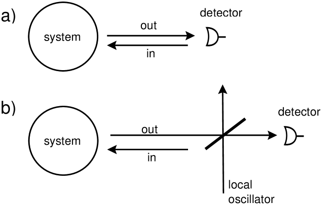
Figure 2: (a) Photon counting, and (b) homodyne detection.

We consider a system which is coupled to $j=1,\ldots,{N_{c}}$ output channels with counters which act continuously to register arrival of photons. A complete description of counting process is given by the family of exclusive probability densities (EPDs):

• $P_{t_{0}}^{t}(0|\rho)$ = probability of having no count in the time interval $(t_{0},t]$ when the system is prepared in the state $\rho$ at time $t_{0}$.

• $p_{t_{0}}^{t}(j_{m},t_{m};\ldots;j_{1},t_{1}|\rho)=$ multitime probability density of having a count in detector $j_{1}$ at time $t_{1}$, a count in detector $j_{2}$ at time $t_{2}$ etc. and no other counts in the rest of the time interval $(t_{0},t]$ (with $j_{k}=1,\ldots,{N_{c}}$; $t_{0}<t_{1}<\ldots<t_{m}\leq t$).

Knowledge of EPDs allows the reconstruction of the whole counting statistics.

Mandel’s counting formula

Physically, the operator for the output current of a photodetector is proportional to the photon flux. To simplify notation we restrict ourselves in the following to the case of a single output channel ${N_{c}}=1$. Furthermore, since the aim of the present discussion is to discuss the relation with the stochastic Schrödinger equation, we will concentrate on the case of ideal photodetection with unit efficiency. The photon flux operator is

$$d\Lambda^{\rm out}(t)\equiv b^{\rm out}(t)^{\dagger}b^{\rm out}(t)\;dt\,=:\,{\hat{I}}(t)\;dt\;.$$ (77)

Here $\Lambda^{\rm out}(t)$ is the operator corresponding to the number of photons up to time $t$ in the out field. We note that the operators $\Lambda^{\rm out}(t)$ are a family of commuting selfadjoint operators. Photoelectric detection realizes a measurement of the compatible observables $\Lambda^{\rm out}(t)$. In quantum optics the usual starting point is the photon counting formulas first derived by Kelley and Kleiner, Glauber and Mandel [3]:

$$P_{m}(t,t_{0})=\left\langle:\frac{1}{m!}\left(\int_{t_{0}}^{t}ds\,{\hat{I}}(s)\right)^{m}\exp\left(-\int_{t_{0}}^{t}ds\,{\hat{I}}(s)\right):\right\rangle\;$$ (78)

gives the probability for $m$ photoncounts in the time interval $(t_{0},t)$ where $:\ldots:$ indicates normal ordering, and $\left\langle\ldots\right\rangle={\rm Tr}_{S\oplus B}\{\ldots{\hat{\rho}}_{0}\}$ with ${\hat{\rho}}_{0}=\rho\otimes|\rm vac\rangle\langle\rm vac|$ is the quantum expectation value with respect to the state of the system. Eq. (78) is valid for a detector with unit efficiency. In particular, the probability of no count in a time interval $(t_{0}=0,t]$ is

$$P_{t_{0}=0}^{t}(0|\rho)=\left\langle:\exp\left(-\int_{0}^{t}ds{\hat{I}}(s)\right):\right\rangle\;,$$ (79)

and the multitime probability density for detecting (exactly) $m$ photons at times $t_{1},\ldots,t_{m}$ in the time interval $(t_{0}=0,t]$ is

$$p_{t_{0}=0}^{t}(t_{m},\dots,t_{1}|\rho)=\left\langle:{\hat{I}}(t_{1})\ldots{\hat{I}}(t_{m})\exp\left(-\int_{0}^{t}ds{\hat{I}}(s)\right):\right\rangle\;.$$ (80)

This establishes the relation to the EPDs introduced above.

On the other hand, the non–exclusive multitime probability density for detecting a first photon at time $t_{1}$, a second (not necessarily the next) photon at time $t_{2}$ etc. and the $m$–th photon at $t_{m}$ is given by the intensity correlation function

$$\left\langle:{\hat{I}}(t_{1})\ldots{\hat{I}}(t_{m}):\right\rangle\;.$$ (81)

The characteristic functional and system averages

As a next step we wish to express the out field correlation functions in terms of system averages. The standard approach is to express in Eqs. (79) and (80) the out field in terms of the in field plus the source contribution, $b^{\rm out}(t)=b^{\rm in}(t)+c(t)$, and to prove and apply the quantum fluctuation regression theorem (QFRT) to evaluate the normally- and time-ordered multitime correlation function for the source operator $c(t)$ [2]. Instead we will follow here the elegant procedure outlined by Barchielli [10, 11] of defining and evaluating a characteristic functional for the EPDs.

We define a characteristic functional as the expectation value of the characteristic operator ${\hat{V}}^{\rm out}_{t}[k]$ according to

$$\Phi_{t}[k] = \left\langle{\hat{V}}^{\rm out}_{t}[k]\right\rangle\quad\mbox{with}\quad{\hat{V}}^{\rm out}_{t}[k]:=\exp\left(i\int_{0}^{t}k(s)\,{\hat{I}}(s)\,ds\right)\;.$$ (82)

When we use the normal ordering relation [5]

$$\exp\left(i\int_{0}^{t}k(s)\,{\hat{I}}(s)\,ds\right)=:\exp\left(\int_{0}^{t}(e^{ik(s)}-1)\,{\hat{I}}(s)\,ds\right):\;,$$ (83)

expand the exponential, and use expressions (79) and (80) we obtain

$$\Phi_{t}[k]:=P_{0}^{t}(0|\rho)+\sum_{m=1}^{\infty} \int_{0}^{t}dt_{m}\int_{0}^{t_{m}}dt_{m-1}\ldots\int_{0}^{t_{2}}dt_{1}$$ (84)

$$\exp\left(i\sum_{r=1}^{m}k(t_{r})\right)p_{0}^{t}(t_{m},\dots,t_{1}|\rho)$$

which relates the characteristic functional to the exclusive probability densities. Thus $\Phi_{t}[k]$ determines uniquely the whole counting process up to time $t$. Functional differentiation of $\Phi_{t}[k]$ with respect to the test functions $k(t)$ gives the moments, correlation functions and counting distributions.

According to Eq. (69) the out and in processes are related by $\Lambda^{\rm out}(t)=U(t)^{\dagger}\Lambda(t)U(t)$ and the characteristic operator satisfies the QSDE

$$d{\hat{V}}^{\rm out}_{t}[k]={\hat{V}}^{\rm out}_{t}[k]\,\left(e^{ik(t)}-1\right)d\Lambda^{\rm out}(t)\quad({\hat{V}}^{\rm out}_{0}[k]=\hat{1}),$$ (86)

$$d\Lambda^{\rm out}(t)=d\Lambda(t)+c(t)\,dB(t)^{\dagger}+c(t)^{\dagger}\,dB(t)+c(t)^{\dagger}c(t)\,dt\;.$$

In a similar way we can express the characteristic operator for the out field in terms of the in field;

$${\hat{V}}^{\rm out}_{t}[k] = U(t)^{\dagger}\exp\left(i\int_{0}^{t}k(s)\,d\Lambda(s)\right)U(t)$$

$$\equiv U(t)^{\dagger}{\hat{V}}_{t}[k]U(t)\;.$$

This allows us to write

$$\Phi_{t}[k] = {\rm Tr}_{S\oplus B}\{{\hat{V}}_{t}[k]\,U(t){\hat{\rho}}(0)U(t)^{\dagger}\}$$ (88)

$$= {\rm Tr}_{S}{\chi}_{t}[k]\quad\mbox{with}\quad{\chi}_{t}[k]:={\rm Tr}_{B}\{{\hat{V}}_{t}[k]\,{\hat{\rho}}(t)\}\;.$$ (89)

which expresses the characteristic functional as the system trace over a characteristic density-like operator $\chi_{t}[k]$ in the system space. Using QSC we can derive an equation for ${\hat{V}}_{t}[k]\,{\hat{\rho}}(t)$,

$$d[{\hat{V}}_{t}[k]\;{\hat{\rho}}(t)]=d{\hat{V}}_{t}[k]\;{\hat{\rho}}(t)+{\hat{V}}_{t}[k]\;d{\hat{\rho}}(t)+d{\hat{V}}_{t}[k]\;d{\hat{\rho}}(t)$$ (90)

with $d{\hat{\rho}}(t)$ from (0.3.3), and ${\hat{V}}_{t}[k]$ obeys an equation similar to (86). Taking the trace over the bath, ${\rm Tr}_{B}\{\ldots\}$, as in the derivation of the reduced density matrix (0.3.3), we obtain the following equation for the characteristic reduced density operator

$$\frac{d}{dt}{\chi}_{t}[k]=\left({\cal L}+(e^{ik(t)}-1){\cal J}\right){\chi}_{t}[k]\quad(\chi_{0}[k]=\rho)\;,$$ (91)

with ${\cal L}$ the Liouville operator from Eq. (0.3.3), and $\cal J$ the “recycling operator” (56). Note that for $k(t)=0$ this characteristic density operator coincides with the system density operator, $\chi_{t}[k=0]=\rho(t)$, and Eq. (91) reduces to the master equation (0.3.3).

We solve Eq. (91) by iteration

$$\chi_{t}[k]={\cal S}(t,0)\rho+\sum_{m=1}^{\infty} \int_{0}^{t}dt_{m}\int_{0}^{t_{m}}dt_{m-1}\ldots\int_{0}^{t_{2}}dt_{1}\exp\left(i\sum_{r=1}^{m}k(t_{r})\right)$$

$${\cal S}(t,t_{m}){\cal J}(t_{m}){\cal S}(t_{m},t_{m-1})\ldots{\cal S}(t_{2},t_{1}){\cal J}(t_{1}){\cal S}(t_{1},0){\rho}$$

with propagators

$${\cal S}(t,t_{0})\rho=U_{\rm eff}(t,t_{0})\rho U_{\rm eff}^{\dagger}(t,t_{0})\quad(t\geq t_{0}),$$ (92)

$${\dot{U}}_{\rm eff}(t,t_{0})=-iH_{\rm eff}(t)U_{\rm eff}(t,t_{0})\quad(U_{\rm eff}(t_{0},t_{0})=\hat{1})\;.$$ (93)

Taking a trace over the system degrees of freedom, and comparing with (84) we can express the EPDs in terms of system averages

$$P_{0}^{t}(0|{\rho})={\rm Tr}_{S}\{{\cal S}(t,0){\rho}\},$$ (94)

$$p_{0}^{t}(t_{1},t_{2},\ldots,t_{m}|{\rho})=$$

$$\quad{\rm Tr}_{S}\{{\cal S}(t,t_{m}){\cal J}(t_{m}){\cal S}(t_{m},t_{m-1})\ldots{\cal S}(t_{2},t_{1}){\cal J}(t_{1}){\cal S}(t_{1},0){\rho}\}\;.$$

The structure of these expressions agrees with what is expected from continuous measurement theory according to Srinivas and Davies [16].

Generalization to many channels

As a reference for the following sections, we give the generalization of these equations to ${N_{c}}$ channels:

$$P_{t_{0}=0}^{t}(0|\rho)={\rm Tr}_{S}\left\{{\cal S}(t,0)\rho\right\}\,,$$ (95)

$$p_{t_{0}=0}^{t}(j_{1},t_{1};\ldots;j_{m},t_{m}|\rho)=$$

$$\quad{\rm Tr}_{S}\left\{{\cal S}(t,t_{m}){\cal J}_{j_{m}}(t_{m}){\cal S}(t_{m},t_{m-1})\ldots{\cal S}(t_{2},t_{1}){\cal J}_{j_{1}}(t_{1}){\cal S}(t_{1},0)\rho\right\}$$

where $t_{0}=0<t_{1}<\ldots\ t_{m}\leq t$ and $j_{k}=1,\ldots,{N_{c}}$.

Examples of the use of the characteristic functional

We conclude our discussion with a few examples for the application of the characteristic functional: The mean intensity of the outgoing field is

$$\left\langle{\hat{I}}(t)\right\rangle=-i\frac{\delta}{\delta k(t)}\Phi_{T}[k]|_{k=0}={\rm Tr}_{S}\{{\cal J}{\rho}(t)\}\quad\mbox{(T > t)}.$$ (96)

The intensity correlation function can be written as the sum of a normally ordered contribution plus a shot noise term

$$\left\langle{\hat{I}}(t){\hat{I}}(t^{\prime})\right\rangle = \left\langle:{\hat{I}}(t){\hat{I}}(t^{\prime}):\right\rangle+\delta(t-t^{\prime})\,\left\langle{\hat{I}}(t)\right\rangle$$

$$= (-i)^{2}\frac{\delta^{2}}{\delta k(t)\,\delta k(t^{\prime})}\Phi_{T}[k]|_{k=0}$$

$$= {\rm Tr}\{{\cal J}(t){\cal T}(t,t^{\prime}){\cal J}(t^{\prime}){\rho}(t^{\prime})\}+\delta(t-t^{\prime}){\rm Tr}_{S}\{{\cal J}(t){\rho}(t)\}\;.$$

The normally ordered $m$-th order intensity correlation function is

$$\left\langle:{\hat{I}}(t_{1})\ldots{\hat{I}}(t_{m}):\right\rangle={\rm Tr}_{S}\{{\cal J}(t_{m}){\cal T}(t_{m},t_{m-1})\ldots{\cal T}(t_{2},t_{1}){\cal J}(t_{1}){\cal T}(t_{1},0){\rho}\}$$ (98)

with ${\cal T}(t,t_{0})=\exp{\cal L}(t-t_{0})$ the time evolution operator for the density matrix according to the master equation.

0.4.2 Conditional Dynamics and A Posteriori States

If during a continuous measurement a certain trajectory of a measured observable is registered, the state of the system conditional to this information is called a conditional state or a posteriori state denoted by $\rho_{c}(t)$, and the corresponding dynamics is referred to as conditional dynamics [3, 12, 14, 15]. In the present case of photodetection (counting processes) we assume that the counters have registered in the time interval $(t_{0}=0,t]$ the sequence $j_{1},t_{1};\ldots;j_{n},t_{n}$ ($t_{1}<\ldots<t_{n}$). To derive an expression for $\rho_{c}(t)$ Barchielli and Belavkin [12] consider

$$P(0,(t,t+{\bar{t}}\,]|\rho)=\frac{p_{0}^{t+\bar{t}}\,(j_{1},t_{1};\ldots;j_{n},t_{n}|\rho)}{p_{0}^{t}(j_{1},t_{1};\ldots;j_{n},t_{n}|\rho)}$$ (99)

which is the conditional probability of observing no count in $(t,t+\bar{t}\,]$ given $\rho$ at time $t_{0}=0$ and having observed the sequence $j_{1},t_{1};\ldots;j_{n},t_{n}$. Obviously one can write $P(0,(t,t+{\bar{t}}]|\rho)=P_{t}^{t+\bar{t}}(0|\rho_{c}(t))$ with

$$\rho_{c}(t)={\cal S}(t,t_{n}){\cal J}_{j_{n}}(t_{n}){\cal S}(t_{n},t_{n-1})\ldots{\cal S}(t_{2},t_{1}){\cal J}_{j_{1}}(t_{1}){\cal S}(t_{1},0)\rho/{\rm Tr}_{S}\{\ldots\}$$ (100)

where ${\rm Tr}_{S}\{\ldots\}$ is a normalization factor to ensure ${\rm Tr}_{S}\rho_{c}(t)=1$. Similar arguments can be given for other EPDs. Thus we identify (100) with the a posteriori state.

Discussion [3, 12, 14, 15]:

• The interpretation of Eq. (100) is as follows: When no count is registered the system evolution is given by ${\cal S}(t,t_{0})$ and the state of the system between two counts is

  $$\rho_{c}(t)={\cal S}(t,t_{r})\rho_{c}(t_{r})/{\rm Tr}_{S}\{{\cal S}(t,t_{r})\rho_{c}(t_{r})\}\quad\mbox{($t\geq t_{r}$)}$$ (101)

  where $t_{r}$ is the time of the last count, and $\rho_{c}(t_{r})$ is the state of the system just after this count.

  When a count $j$ at time $t=t_{r}$ is registered the action on the system is given by the operator ${\cal J}_{j}$, and the state of the system immediately after is

  $$\rho_{c}(t_{r}+dt)={\cal J}_{j}(t_{r})\rho_{c}(t_{r})/{\rm Tr}_{S}\{{\cal J}_{j}(t_{r})\rho_{c}(t_{r})\}\;.$$ (102)

  We will call this a “quantum jump.”

• When the system is initially in a pure state described by the state vector $\psi$, $\rho=|\psi\rangle\langle\psi|$, it will remain in a pure state $\psi_{c}(t)$, $\rho_{c}(t)=|\psi_{c}(t)\rangle\langle\psi_{c}(t)|$. The time evolution between the counts is

  $${\tilde{\psi}}_{c}(t)=U_{\rm eff}(t,t_{r}){\tilde{\psi}}_{c}(t_{r}),\quad\psi_{c}(t)={\tilde{\psi}}_{c}(t)/|\!|{\tilde{\psi}}_{c}(t)|\!|$$ (103)

  i.e.

  $$\frac{d}{dt}{\tilde{\psi}}_{c}(t)=-iH_{\rm eff}{\tilde{\psi}}_{c}(t)$$ (104)

  where ${{\tilde{\psi}}_{c}(t)}$ and ${\psi_{c}(t)}$ denotes the unnormalized and normalized wave functions, respectively, and a count $j,t_{r}$ is associated with the quantum jump

  $${\tilde{\psi}}_{c}(t_{r}+dt)=\lambda_{j}{c}_{j}{\tilde{\psi}}_{c}(t_{r})\;.$$ (105)

  The complex numbers $\lambda_{j}\neq 0$ (with dimension $[\mbox{\rm time}]^{1/2}$) are arbitray and can be chosen, for example, to renormalize the wave function ${\tilde{\psi}}_{c}(t)$ after the jump.

• In preparation for the wavefunction simulation to be discussed in Sec.0.4.3 we note: The mean number of counts of type $j$ in the time interval $(t,t\!+\!dt]$ conditional upon the observed trajectory $j_{1},t_{1};\ldots;j_{n},t_{n}$ is

  $$p_{t}^{t\!+\!dt}(j,t|\rho_{c}(t))\>dt=\left\{\begin{array}[]{ll}{\rm Tr}_{S}\{{\cal J}_{j}(t)\rho_{c}(t)\}\>dt&\\ |\!|{c}_{j}\psi_{c}(t)|\!|^{2}\>dt&\end{array}\right.\;,$$ (106)

  and the joint probability that no jump occured in the time interval $(0,t]$, and a jump of type $j$ occured in $(t,t\!+\!dt]$ given $\rho$ at time $t=0$ is

  $$p_{t}^{t\!+\!dt}(j,t|\;\rho_{c}(t)\;)\times P_{0}^{t}(0|\rho)=\left\{\begin{array}[]{ll}{\rm Tr}_{S}\{{\cal J}_{j}(t){\cal S}(t,0)\rho\}\>dt&\\ |\!|{c}_{j}\,U_{\rm eff}(t,0)\psi|\!|^{2}\>dt&\end{array}\right.\;.$$ (107)

  with $\rho_{c}(t)={{\cal S}(t,0)\rho/{\rm Tr}_{S}\{{\cal S}(t,0)\rho\}}$.

0.4.3 Stochastic Schrödinger Equation and Wave Function Simulation for Counting Processes

Stochastic Schrödinger Equation

We can combine the time evolution for the (unnormalized) conditional wave function ${\tilde{\psi}}_{c}(t)$ according to Eqs. (103,104) into a single (c–number) Stochastic Schrödinger Equation (SSE) [12, 15]. A typical trajectory $N_{j}{(t)}$, where $N_{j}{(t)}$ is the number of counts up to time $t$, $j=1,\ldots,{N_{c}}$ is a sequence of step functions, such that $N_{j}{(t)}$ increases by one if there is a count of type $j$ and $N_{j}{(t)}$ is constant otherwise. Therefore, the Ito differential

$$dN_{j}{(t)}\equiv N_{j}{(t\!+\!dt)}-N_{j}{(t)}=\left\{\begin{array}[]{ll}1&\mbox{if count $j$ in $(t,t\!+\!dt]$}\\ 0&\mbox{else}\end{array}\right.$$ (108)

fulfills $[dN_{j}{(t)}]^{2}=dN_{j}{(t)}$. Moreover the probability of more than one count in an interval $dt$ vanishes faster than $dt$. We thus have the Ito table

$$dN_{j}{(t)}\;dN_{k}{(t)}=\delta_{jk}\;dN_{j}{(t)},\quad dN_{j}{(t)}\>dt=0$$ (109)

and obtain a Stochastic Schrödinger Equation for the unnormalized wave function ${\tilde{\psi}}_{c}(t)$

$$d{\tilde{\psi}}_{c}(t) \equiv {\tilde{\psi}}_{c}(t\!+\!dt)-{\tilde{\psi}}_{c}(t)$$

$$= \left\{-iH_{\rm eff}\>dt+\sum_{j=1}^{N_{c}}\left(\lambda_{j}{c}_{j}-\hat{1}\right)dN_{j}{(t)}\right\}{\tilde{\psi}}_{c}(t)\;$$

with $\lambda_{j}\neq 0$. According to (106) the mean number of counts of type $j$ in the interval $(t,t\!+\!dt]$ conditional to the trajectory $j_{1},t_{1};\ldots;j_{n},t_{n}$ (indicated by the subscript $c$) is

$$\left\langle dN_{j}{(t)}\right\rangle_{c}=|\!|{c}_{j}\psi_{c}(t)|\!|^{2}\>dt\;.$$ (111)

The SSE (0.4.3) can be converted to an equation for the normalized $\psi_{c}(t)={\tilde{\psi}}_{c}(t)/|\!|{\tilde{\psi}}_{c}(t)|\!|$. As an illustration for Ito calculus we give details in Appendix .6. The result is

$$d\psi_{c}(t) \equiv \psi_{c}(t\!+\!dt)-\psi_{c}(t)$$

$$= \Big{\{}-iH\,dt-\frac{1}{2}\sum_{j=1}^{N_{c}}\left({c}_{j}^{\dagger}{c}_{j}-\left\langle{c}_{j}^{\dagger}{c}_{j}\right\rangle_{c}\right)\;dt$$

$$+\sum_{j=1}^{N_{c}}\left({c}_{j}/\sqrt{\left\langle{c}_{j}^{\dagger}{c}_{j}\right\rangle_{c}}-1\right)dN_{j}{(t)}\Big{\}}\psi_{c}(t)\;.$$

where

$$\left\langle\ldots\right\rangle_{c}=\langle\psi_{c}(t)|\ldots|\psi_{c}(t)\rangle\;.$$ (113)

Eq. (0.4.3) is a nonlinear Schrödinger equation. (Note: Eq. (0.4.3) is not unique up to a phase factor: $\psi_{c}(t)\rightarrow e^{i\phi(t)}\psi_{c}(t)$ where $\phi(t)$ is solution of a stochastic differential equation $d\phi(t)=a(t)\>dt+\sum b_{j}(t)dN_{j}{(t)}$ with arbitrary $a(t)$ and $b_{j}(t)$.)

Equation of motion for the Stochastic Density Matrix

Finally, we derive an equation for the Stochastic Density Matrix $\rho_{c}(t)=|\psi_{c}(t)\rangle\langle\psi_{c}(t)|$,

$$d\rho_{c}(t) \equiv \rho_{c}(t\!+\!dt)-\rho_{c}(t)$$

$$= {\cal L}\rho_{c}(t)\>dt+\sum_{j=1}^{N_{c}}\left(\frac{{\cal J}_{j}\rho_{c}(t)}{{\rm Tr}_{S}\{{\cal J}_{j}\rho_{c}(t)\}}-\rho_{c}(t)\right)\left(dN_{j}{(t)}-\right.$$

$$\left.{\rm Tr}_{S}\{{\cal J}_{j}\rho_{c}(t)\}\>dt\right)\;.$$

Discussion: The Master Equation (58) is (re)derived by taking the stochastic mean of Eq. (0.4.3). We first take the mean for the time step $t\rightarrow t\!+\!dt$ conditional upon a given trajectory. All quantities on the right hand side of Eq. (0.4.3) depend only on the past (they are nonanticipating or adapted functions), but the a posteriori mean value of $\left\langle dN_{j}{(t)}\right\rangle_{c}$ is given by (111), and thus the last term vanishes. Then we take mean values also on the past, and obtain the master equation (58): $\dot{\rho}(t)={\cal L}\rho(t)$. Thus, if the results of a measurement are not read, i.e. no selection is made, the state of the system at time $t$ will be $\rho(t)=\left\langle\rho_{c}(t)\right\rangle_{\rm st}$, and $\rho(t)$ is the a priori state for the case of continuous measurement.

From our construction it is obvious that the statistics of the jumps $N_{j}(t)$ is identical to the statistics of photon counts discussed in Sec. 0.4.1. However, as a consistency check and for pedagogical purposes, we will rederive the counting statistics in the framework of the characteristic functional for the counting process $N_{j}(t)$ and show that it is identical to the characteristic functional derived in Sec. 0.4.1. We confine ourselves to ${N_{c}}=1$. In the present context the charcteristic functional for the counting process $N_{1}(t)\equiv N(t)$ is defined as

$$\Phi_{t}[k]=\left\langle V_{t}[k]\right\rangle_{\rm st}\mbox{with}\quad V_{t}[k]:=\exp\left(i\int_{0}^{t}k(s)\,dN{(s)}\right)\;$$ (115)

which should be compared with the definition (82) for the output operator $\Lambda^{\rm out}(t)$. The quantity $V_{t}[k]$ satisfies the c–number SDE

$$dV_{t}[k]=V_{t}[k]\,\left(e^{ik(t)}-1\right)dN{(t)}\;.$$ (116)

In analogy to Eq. (88) we introduce

$$\Phi_{t}[k]={\rm Tr}_{S}\chi_{t}[k]\quad\mbox{with}\quad\chi_{t}[k]:=\left\langle V_{t}[k]\,\rho_{c}(t)\right\rangle_{\rm st}\;.$$ (117)

According to Ito calculus

$$d[V_{t}[k]\;\rho_{c}(t)]=dV_{t}[k]\;\rho_{c}(t)+V_{t}[k]\;d\rho_{c}(t)]+dV_{t}[k]\;d\rho_{c}(t)$$ (118)

where $dV_{t}[k]$ and $d\rho_{c}(t)$ obey Eqs. (116) and (0.4.3), respectively. Repeating the arguments given in the derivation of the density matrix equation from the stochastic density matrix equation given above, we take a stochastic average $\left\langle\ldots\right\rangle_{\rm st}$ of the equation for $V_{t}[k]\;\rho_{c}(t)$ and find that $\chi_{t}[k]\equiv\left\langle V_{t}[k]\;\rho_{c}(t)\right\rangle_{\rm st}$ (Eq. (117)) satisfies the equation of motion and initial condition (91) given in Sec. 0.4.1. This completes the proof that the characteristic functional defined in Eq. (115) is identical to the characteristic functional of Sec. 0.4.1.

A direct derivation of the c–number SSE (0.4.3) from the QSSE (51) has been given by Gardiner et al.  [14]. Goetsch and Graham [17] have given a derivation by working with a eigenrepresentation of the set of commuting operators $d\Lambda(t)$.

Wave Function Simulation

The conditional dynamics defined by Eqs. (103,105) together with (107) suggests a wave function simulation of the reduced system density matrix $\rho(t)$ as follows [3, 11, 12, 14, 15, 17, 18, 19, 20, 21, 23, 24, 25, 26, 27, 28, 29, 30, 31, 32, 33, 34]:

• We choose a system wave function ${\tilde{\psi}}_{c}(t_{0})$, initially normalized $|\!|{\tilde{\psi}}_{c}(t_{0})|\!|=1$, and set the counter $n$ for the number of quantum jumps equal to zero, $n=0$.

• We propagate the (unnormalized) conditional wavefunction ${\tilde{\psi}}_{c}$ according to Eq. (103) and simulate the time $t$ and type of count $j$ of the next quantum jump according to the conditional density (107),

  $$\tilde{c}(j,t)=|\!|c_{j}{\tilde{\psi}}_{c}(t)|\!|^{2}\quad\mbox{($t\geq t_{n},|\!|{\tilde{\psi}}_{c}(t_{n})|\!|=1$)}.$$ (119)

• • Note: One possible way to determine $t$ and $j$ is to proceed in two steps. First, we find a decay time $t$ according to the delay function $\tilde{c}(t)=\sum_{j}\tilde{c}(j,t)$. This is conveniently done by drawing a random number $0\leq r\leq 1$ from a uniform distribution and monitoring the norm of ${\tilde{\psi}}_{c}(t)$ until

    $$\int^{t}_{t_{n}}dt^{\prime}\tilde{c}(t^{\prime}) \equiv 1-|\!|{\tilde{\psi}}_{c}(t)|\!|^{2}$$

    $$= r\;\epsilon\;[0,1]\;\quad\mbox{($t\geq t_{n}$; $|\!|{\tilde{\psi}}_{c}(t_{n})|\!|=1$).}$$

    Second, the type of count $j$ is determined from the conditional density $\tilde{c}(j|t)=\tilde{c}(j,t)/\sum_{k}\tilde{c}(k,t)$ for the given time $t$.

  Incrementing $n\rightarrow n+1$ we identify $t_{n}\equiv t$ and $j_{n}\equiv j$ with the decay time and type of count, respectively. The wave function after the quantum jump is given by Eq. (105). We renormalize this wavefunction and continue integrating (103) up to the next jump time, i.e. return to the beginning of Step B.

• An approximation for the system density matrix is obtained by repeating these simulations in steps A and B to obtain

  $$\rho(t)=\left\langle|\psi_{c}(t)\rangle\langle\psi_{c}(t)|\right\rangle_{\rm st}$$ (121)

  where $\left\langle\ldots\right\rangle_{\rm st}$ denotes an average over the different realizations of system wave functions.

Remarks:

• A simulation of the quantum master equation in terms of system wave functions can replace the solution of the master equation for the density matrix, and an important feature of the wave function approach, first emphasized by Dalibard, Castin and Mølmer [18], is that one has only to deal with a wave function of dimension $N$, as opposed to working with the density matrix and its $N^{2}$ elements. Thus, simulations can provide solutions when a direct solution of the master equation is impractical because of the large dimension of the system space. Convergence of the simulation vs. a direct solution of the master equation in terms of “global” and “local” observables are given in Ref. [19].

  In many problems one is interested in a steady state density matrix. In this case it is often convenient to replace the ensemble averages by the time average of a single trajectory.

  A simulation has the further advantage that it allows the calculations to be performed on a distributed system of networked computers [26], with a corresponding gain in computational power. In view of the statistical independence of the different wavefunction realizations, parallelization of the algorithm is trivial.

• The ${N_{c}}$–channel master equation (58) is form invariant under the transformation

  $${c}_{j}\rightarrow\sum_{k=1}^{N_{c}}U_{jk}{c}_{k}\quad\mbox{where }(\sum_{j=1}^{N_{c}}U_{jk}U_{lk}^{*}=\delta_{jl})$$ (122)

  (that is with $U$ a unitary matrix). The decomposition of Eq. (58) to form quantum trajectories ${\tilde{\psi}}_{c}(t)$ is thus not unique. Different sets of jumps operators $\{{c}_{j}\}$ not only lead to a different physical interpretation of trajectories, but an appropriate choice of ${c}_{j}$ may be crucial for the formulation of an efficient simulation method for estimating the ensemble distribution. An example will be given in Sec. 0.5.2 [43] (see also [19]).

• Any master equation conforming to the requirements for $\rho$ is of the Lindblad form [2]

  $${\dot{\rho}}=-i[H,\rho]+\sum_{i,j=1}^{{N_{c}}}\gamma_{ij}\left(2{c}_{i}\rho{c}_{j}^{\dagger}-{c}_{j}^{\dagger}{c}_{i}\rho-\rho{c}_{j}^{\dagger}{c}_{i}\right)\;.$$ (123)

  This can be brought into the form (58) by diagonalizing the Hermitian matrix $\gamma_{ij}$ by a unitary transformation $V_{i\gamma}$,

  $$\gamma_{ij}=\sum_{\gamma=1}^{{N_{c}}}V_{i\gamma}\kappa_{\gamma}(V_{\gamma i})^{\dagger}\quad\mbox{($i,j,=1,\ldots,{N_{c}}$)}$$ (124)

  with eigenvalues $\kappa_{\gamma}\geq 0$, and defining

  $${c}_{\gamma}=\sqrt{\kappa_{\gamma}}\sum_{i=1}^{{N_{c}}}{c}_{i}V_{i\gamma}\;.$$ (125)

  Applications of this procedure to the master equation for squeezed noise can be found in Ref. [21].

0.4.4 Simulation of Stationary Two-Time Correlation Functions

We are often interested in system correlation functions $\left\langle A(t)B({t_{0}})\right\rangle$ and their Fourier transform (spectra) (see section 0.5.2). According to the quantum fluctuation regression theorem the system correlation function can be written as

$$\left\langle A(t)B({t_{0}})\right\rangle={\rm Tr}_{S}\{Ae^{{\cal L}(t-{t_{0}})}B\rho({t_{0}})\}\quad(t\geq{t_{0}})\;.$$ (126)

This correlation function can be obtained by solving the density matrix equation for $\rho(t)$ and an equation for the first order response $\rho^{(+)}(t)$

$${\dot{\rho}}(t)={\cal L}\rho(t),$$ (127)

$${\dot{\rho}}^{(+)}(t)={\cal L}\rho^{(+)}(t)+Bf(t)\rho(t)\;.$$ (128)

By formally integrating Eq. (128),

$$\rho^{(+)}(t)=\int^{t}dt_{1}e^{{\cal L}(t-t_{1})}Bf(t_{1})\rho(t_{1})$$ (129)

and choosing a $\delta$–function $f(t)=\delta(t-{t_{0}})$ we have

$${\rm Tr}_{S}\{A\rho^{(+)}(t)\}=\left\langle A(t)B({t_{0}})\right\rangle\quad(t\geq{t_{0}})\;.$$ (130)

We will show that these correlation functions can be obtained by solving (simulating) the set of stochastic Schrödinger equations [14, 21, 26]

$$d{\tilde{\psi}}_{c}(t)=\left[-iH_{\rm eff}\>dt+\sum_{j=1}^{d}(\lambda_{j}{c}_{j}-\hat{1})dN_{j}{(t)}\right]{\tilde{\psi}}_{c}(t)$$ (131)

$$d{\tilde{\psi}}_{c}^{(+)}(t)=\left[-iH_{\rm eff}\>dt+\sum_{j=1}^{d}(\lambda_{j}{c}_{j}-\hat{1})dN_{j}{(t)}\right]{\tilde{\psi}}_{c}^{(+)}(t)+f(t)B{\tilde{\psi}}_{c}(t)dt$$

with quantum jumps dictated by ${\tilde{\psi}}_{c}(t)$ according to $\left\langle dN_{j}{(t)}\right\rangle_{c}=|\!|{c}_{j}\psi_{c}(t)|\!|^{2}\>dt$. For a $\delta$–kick ${\tilde{\psi}}_{c}^{(+)}(t)$ obeys the same Schrödinger equation as ${\tilde{\psi}}_{c}(t)$ (Eq. (131)), where the inhomogeneous term in (0.4.4) translates into the initial condition

$${\tilde{\psi}}_{c}^{(+)}({t_{0}}+dt)=B{\tilde{\psi}}_{c}({t_{0}})\;.$$ (132)

It is straightforward to show that the stochastic averages

$$\rho(t)=\left\langle|{\tilde{\psi}}_{c}(t)\rangle\langle{\tilde{\psi}}_{c}(t)|/|\!|{\tilde{\psi}}_{c}(t)|\!|^{2}\right\rangle_{\rm st}$$ (133)

$$\rho^{(+)}(t)=\left\langle|{\tilde{\psi}}_{c}^{(+)}(t)\rangle\langle{\tilde{\psi}}_{c}(t)|/|\!|{\tilde{\psi}}_{c}(t)|\!|^{2}\right\rangle_{\rm st}$$ (134)

(both normalized with respect to ${\tilde{\psi}}_{c}(t)$) obey Eqs. (127, 128), and thus

$$\left\langle A(t)B({t_{0}})\right\rangle=\big{\langle}\;\left\langle\langle{\tilde{\psi}}_{c}(t)|A|{\tilde{\psi}}_{c}^{(+)}(t)\rangle/|\!|{\tilde{\psi}}_{c}(t)|\!|^{2}\right\rangle_{\rm st}\;\big{\rangle}_{{t_{0}}}$$ (135)

where $\left\langle\ldots\right\rangle_{{t_{0}}}$ indicates an average over radmonly selected initial “kick”–times $t_{0}$. A physical interpretation of this procedure is summarized in the discussion following Eq. (169). The above derivation emphasizes the simulation of a correlation function. We can simulate a spectrum directly when instead of the $\delta$-kick we use a function $f(t)\propto\exp\left(-i\nu t\right)$ [14, 21, 22, 26]. For another approach to simulate correlation functions we refer to [19].

0.4.5 Diffusion Processes and Homodyne Detection

Le us consider homodyne detection as shown in Fig. 2b [3, 11, 15]. In the simplest configuration, the output field of the system $b^{\rm out}(t)$ is sent through a beam splitter of transmittance close to one. The other port of the beam splitter is a strong coherent field which serves as a local oscillator. For a single output channel, the transmitted field is then represented by $b^{\rm out}(t)^{\prime}=b^{\rm out}(t)+\gamma={c}+\gamma+b(t)$ . Assuming a real field $\gamma$ the operator for photon counting of the outgoing field is

$$d\Lambda^{\rm out}(t)^{\prime}/dt \equiv b^{\rm out}(t){{}^{\dagger}}^{\prime}b^{\rm out}(t)^{\prime}$$

$$= \gamma^{2}+\gamma\left[c+c^{\dagger}+b(t)+b(t)^{\dagger}\right]+\left[c^{\dagger}+b(t)^{\dagger}\right]\left[c+b(t)\right]\;.$$

The ideal limit of homodyne detection is for infinite amplitude of the local oscillator. Physically, in this limit the count rate of the photodetectors will go to infinity, but we can be define an operator for the homodyne current ${\hat{I}}^{\rm hom}(t)$ by subtracting the local oscillator contribution:

$${\hat{I}}^{\rm hom}(t) = \lim_{\gamma\rightarrow\infty}\frac{d\Lambda^{\rm out}(t)^{\prime}-\gamma^{2}\;dt}{\gamma\;dt}\;.$$ (137)

Defining quadrature operators for the in and out field,

$$d{\hat{X}(t)}:=dB(t)+dB^{\dagger}(t),\quad d{\hat{Y}}(t):=-idB(t)+idB(t)^{\dagger}$$ (138)

and for the system dipole

$$x:=c+c^{\dagger},\quad y:=-ic+ic^{\dagger}\;,$$ (139)

we can write

$$d{\hat{X}}^{\rm out}(t) = {\hat{I}}^{\rm hom}(t)\,dt$$

$$= x(t)\,dt+d{\hat{X}}(t)\;$$

where the second line is the QSDE for the $X$–quadrature of the out–field which follows from Eq. (74). This equation shows that homodyne detection with $\gamma$ real corresponds to a measurement of the compatible observables $b^{\rm out}(t)+b^{\rm out}(t)^{\dagger}=d{\hat{X}}^{\rm out}(t)/dt$ ($t\geq 0$), the quadrature components of the field.

The complete statistics of the homodyne current is obtained from a characteristic functional [11]

$$\Phi_{t}[k] = \left\langle{\hat{V}}^{\rm out}_{t}[k]\right\rangle\quad\mbox{with}\quad{\hat{V}}^{\rm out}_{t}[k]:=\exp\left(i\int_{0}^{t}k(s)\,d{\hat{X}}^{\rm out}(s)\right).$$ (141)

The characteristic operator is determined by the QSDE

$$d{\hat{V}}^{\rm out}_{t}[k]={\hat{V}}^{\rm out}_{t}[k]\,\left(ik(t)\,d{\hat{X}}^{\rm out}(t)-\frac{1}{2}k(t)^{2}\,dt\right)\quad({\hat{V}}^{\rm out}_{0}[k]=\hat{1})$$ (142)

together with Eq. (0.4.5) for $d{\hat{X}}^{\rm out}(t)$. Following the derivations of Sec. 0.4.1 we define a characteristic density operator $\chi_{t}[k]$ which gives the characteristic functional $\Phi_{t}[k]$ (141) according to (88). We obtain the equation

$$\frac{d}{dt}\chi_{t}[k]={\cal L}\chi_{t}[k]-\frac{1}{2}k(t)^{2}\chi_{t}[k]+ik(t)\left(c\chi_{t}[k]+\chi_{t}[k]c^{\dagger}\right)\quad\mbox{where ($\chi_{0}[k]=\rho(0)$)}$$ (143)

corresponding to a Gaussian diffusive measurement [12]. An expression for the mean homodyne current and current - current correlation function will be given below in Eqs. (0.4.6) and (0.4.6), respectively.

0.4.6 Stochastic Schrödinger Equation and Wave Function Simulation for Diffusion Processes

We now turn to a c–number stochastic description and the derivation of a c–number stochastic Schrödinger equation for diffusion processes. Such an equation was first derived by Carmichael [3] (see also [15]) from an analysis of homodyne detection, and independently in a more formal context by Barchielli and Belavkin [12].

From (106) the mean rate of photon counts is

$$\left\langle dN{(t)}\right\rangle_{c} = {\rm Tr}_{S}\{({c}^{\dagger}+\gamma)({c}+\gamma)\rho_{c}(t)\}\>dt$$

$$= {\rm Tr}_{S}\{(\gamma^{2}+\gamma x+{c}^{\dagger}{c})\rho_{c}(t)\}\>dt\;,$$

and registration of a count in homodyne detection is associated with a quantum jump ${\tilde{\psi}}_{c}\leftarrow(c+\gamma){\tilde{\psi}}_{c}$ of the system wave function. Furthermore, we note that the master equation is invariant under the transformation

$${c} \rightarrow {c}+\gamma$$ (145)

$$H \rightarrow H-i\frac{1}{2}(\gamma^{*}{c}-\gamma{c}^{\dagger})$$ (146)

which involves a displacement of the jump operators by a complex number $\gamma$. With these replacments we obtain from the SSE (0.4.3)

$$d\psi_{c}(t) = \left(-iH-\frac{1}{2}\left({c}^{\dagger}{c}+2\gamma{c}-\left\langle{c}^{\dagger}{c}\right\rangle_{c}-\gamma\left\langle x\right\rangle_{c}\right)\right)\>dt\;\psi_{c}(t)$$

$$+ \left(\frac{{c}+\gamma}{\sqrt{\left\langle({c}^{\dagger}+\gamma)({c}+\gamma)\right\rangle_{c}}}-1\right)dN{(t)}\;\psi_{c}(t)$$

We are again interested in the ideal limit when the local oscillator amplitude $\gamma$ goes to infinity. As pointed out before, in the limit that $\gamma$ is much larger than ${c}$, the count rate (0.4.6) consists of a large constant term (the counting rate form the local oscillator), a term proportional to the $x$ quadrature of the system dipole, and a small term, the direct count rate from the system. Subtracting from the counting rate the contribution of the local oscillator we write

$$dN{(t)}=\gamma^{2}\>dt+\gamma\;dX(t)$$ (148)

which defines the stochastic process $X(t)$. For $\gamma\rightarrow\infty$ the stochastic process $X(t)$ has the Gaussian properties

(i) $$\left\langle{d{X{(t)}}}\right\rangle_{c}=\left\langle x\right\rangle_{c}\;dt$$ (149)

(ii) $$[dX(t)]^{2}=\;dt,\quad dX(t)\,dt=0$$ (150)

$$\Longrightarrow dX(t)-\left\langle dX(t)\right\rangle_{c}=dW(t)$$ (151)

where $dW(t)$ is a Wiener increment $[dW(t)]^{2}=dt$, $\left\langle dW(t)\right\rangle_{c}=0$. Thus the jumps (0.4.6) are replaced by a diffusive evolution. The derivation of (149) is straightforward [12]: Eq. (149) follows from Eq. (0.4.6); Eq. (150) is obtained from the Ito table (109), $[dX(t)]^{2}=dN{(t)}/\gamma^{2}=\;dt+{dX(t)}/\gamma$. Physically we interpret

$$I^{\rm hom}(t) = \frac{dX(t)}{dt}\equiv\lim_{\gamma\rightarrow\infty}\frac{dN{(t)}-\gamma^{2}\;dt}{\gamma\;dt}$$

$$= \left\langle x\right\rangle_{c}(t)+\xi(t)$$

as a stochastic homodyne current with $\xi(t)=dW(t)/dt$ white noise.

Taking this limit in Eq. (0.4.6), we obtain a SSE for diffusive processes

$$d\psi_{c}(t) = \Big{\{}\left(-iH-\frac{1}{2}({c}^{\dagger}{c}-\left\langle x\right\rangle_{c}{c}+\frac{1}{4}\left\langle x\right\rangle_{c}^{2})\right)\>dt$$

$$+\left({c}-\left\langle x/2\right\rangle_{c}\right)dW(t)\Big{\}}\psi_{c}(t)\;.$$

Eq. (0.4.6) is not unique; in particular we can make a phase transformation $\psi_{c}(t)\rightarrow e^{i\phi(t)}\psi_{c}(t)$ which allows us to rewrite this equation as [12]

$$d\psi_{c}(t) = \Big{\{}\left(-iH-\frac{1}{2}{c}^{\dagger}{c}+\left\langle{c}^{\dagger}\right\rangle_{c}{c}+\frac{1}{2}|\left\langle{c}\right\rangle_{c}|^{2}\right)\>dt$$

$$+\left({c}-\left\langle{c}\right\rangle_{c}\right)dW(t)\Big{\}}\psi_{c}(t)\;,$$

and there are also versions with complex noises [35, 36, 38].

The unnormalized version of the equation has been given by Carmichael [3], and more recently by Wiseman [15, 17]

$$d{\tilde{\psi}}_{c}(t)=-iH-\frac{1}{2}{c}^{\dagger}{c}+I^{\rm hom}(t)\;{c}]\;dt\;{\tilde{\psi}}_{c}(t)\;$$ (155)

which demonstrates clearly how the state is conditioned on the measured photocurrent $I^{\rm hom}(t)$.

A stochastic density matrix equation for diffusive processes is directly obtained from these equations,

$$d\rho_{c}(t)={\cal L}\rho_{c}\,dt+\left[\left(c-\left\langle c\right\rangle_{c}\right)\rho_{c}+\rho_{c}\left(c^{\dagger}-\left\langle c^{\dagger}\right\rangle_{c}\right)\right]\,dW(t)$$ (156)

and taking stochastic averages we see - as expected - that the a priori dynamics satisfies the master equation (0.3.3).

As shown by Goetsch et al.  [17] the above c–number SSE for diffusive processes can be derived directly from the QSSE (51). The idea is to replace $dB(t)^{\dagger}\,c|\Psi(t)\rangle\rightarrow(dB(t)+dB(t)^{\dagger})\,c|\Psi(t)\rangle\equiv d{\hat{X}}(t)^{\dagger}\,c|\Psi(t)\rangle$ in Eq. (51) and to subsequently project on an eigenbasis of the set of commuting operators $d{\hat{X}}$. Generalization of the SSEs to a squeezed bath have been given in [15, 17].

The stochastic homodyne current $I^{\rm hom}(t)$ (0.4.6) has the same statistical properties as the operator version ${\hat{I}}^{\rm hom}(t)$ as becomes evident by defining a characteristic functional [12]

$$\Phi_{t}[k]=\left\langle V_{t}[k]\right\rangle_{\rm st}\mbox{with}\quad V_{t}[k]:=\exp\left(i\int_{0}^{t}k(s)\,dX(s)\right)$$ (157)

where $V_{t}[k]$ satisfies the SDE

$$dV_{t}[k]=V_{t}[k]\,\left(ik(t)\,dX(t)-\frac{1}{2}k(t)^{2}\,dt\right)\;.$$ (158)

Following (117) we again define a “density matrix” $\chi_{t}[k]$, and use Ito calculus (118) with the above equation for $V_{t}[k]$ and the stochastic density matrix equation for diffusive processes (156) to find that $\chi_{t}[k]$ obeys an equation and initial conditions identical to (143). Thus the characteristic functionals $\Phi_{t}[k]$ defined in Eqs. (141) and (157), respectively, are identical.

As an example, we readily derive the mean homodyne current

$$\left\langle{\hat{I}}^{\rm hom}(t)\right\rangle\equiv\left\langle I^{\rm hom}(t)\right\rangle_{\rm st}=-i\frac{\delta}{\delta k(t)}\Phi_{T}[k]|_{k=0}={\rm Tr}_{S}x\rho(t)$$

and the stationary homodyne correlation function whose Fourier transform gives the spectrum of squeezing [3]

$$\left\langle{\hat{I}}^{\rm hom}(t_{1}){\hat{I}}^{\rm hom}(t_{2})\right\rangle \equiv \left\langle I^{\rm hom}(t_{1})I^{\rm hom}(t_{2})\right\rangle_{\rm st}$$

$$= (-i)^{2}\frac{\delta^{2}}{\delta k(t)\,\delta k(t^{\prime})}\Phi_{T}[k]|_{k=0}$$

$$= {\rm Tr}_{S}\left[xe^{{\cal L}(t_{2}-t_{1})}\left(c\rho+\rho c^{\dagger}\right)\right]+\delta(t_{2}-t_{1})$$

where the last term is the shot noise contribution.

As a final comment we note that a completely different interpretation of the stochastic Schrödinger equations of the type (0.4.6) have been proposed in Refs. [35, 36, 38] in connection with dynamical theories of wave function reduction. The assumption is that the reduction of the wavefunction associated with a measurement is a stochastic process and an equation of the type (0.4.6) is postulated.

There have been numerous applications of the diffusive SSE. A beautiful discussion of squeezing in a parametric amplifier in terms of trajectories can be found in Carmichael’s book [3]. Illustrations for the decay of Schrödinger cats have been given in [17, 32, 33, 44]. A theory of quantum feedback has been developed by Milburn and Wiseman [15].

0.5 Application and Illustrations

During the last years we have seen numerous, mostly numerical applications of the SSE [3, 11, 12, 14, 15, 17, 18, 19, 20, 21, 23, 24, 25, 26, 27, 28, 29, 30, 31, 32, 33, 34]. Roughly speaking, these calculations can be divided into illustrations where single trajectories illustrate certain features of the physics one wishes to discuss, and as a numerical simulation method for situations where a direct solution of the master equation is not feasible. Below we discuss a few examples from our recent work. Our first example is state preparation in ion traps through quantum jumps; the second example is a discussion of simulations in laser cooling, and we conclude with remarks on possible application to the problem of decoherence in quantum computing.

0.5.1 State Preparation by Observation of Quantum Jumps in an Ion Trap

Ions traps provide a tool to store and observe laser cooled single ions for an essentially unlimited time. Experiments with single trapped ions thus represent a realization of continuous observation of a single quantum system in the context of quantum optics. For a review on ion traps and application in quantum optics we refer to [45, 46].

Quantum Jumps in Three-Level Atoms

The probably best-known example is the problem of “observation of quantum jumps in three level system” [42] (for a review and references see [41]). The system of interest involves a double–resonance scheme where two excited states $|e\rangle$ and $|r\rangle$ are connected to a common lower level $|g\rangle$ via a strong and weak transition, respectively. The fluorescent photons from the strong transition are observed. However, an excitation of the weak transition where the electron is temporarily shelved in the metastable state $|r\rangle$ will cause the fluorescence from the strong transition to be turned off. It is, therefore, possible to monitor the quantum jumps of the weak transition via emission windows in the (macroscopic) signal provided by the fluorescence of the strong transition. Experimental observation of this effect has been reported in Refs. [42], and various theoretical treatments of this effect have been published. From a theoretical point of view, the problem is to study the photon statistics of the photons emitted on the strong line of the three–level atom. A treatment based on continuous measurement theory was given by Zoller et al.  [39] and Barchielli [10] (see also [47]): in Ref. [39] the probability density for the “emission of the next photon on the strong line” (delay function) was calculated, and for the first time a simulation of the a posteriori dynamics was described to illustrate the conditional dynamics of a single continuously monitored quantum system.

The master equation for a three–level atom has the form

$${\dot{\rho}}=-i(H_{\rm eff}\rho-\rho H_{\rm eff}^{\dagger})+{\cal J}_{\rm s}\rho+{\cal J}_{\rm w}\rho\quad(\equiv{\cal L}\rho)$$ (160)

where ${\cal J}_{\rm s}\rho:=|g\rangle\langle g|\,\Gamma_{s}\rho_{ee}$ and ${\cal J}_{\rm w}\rho:=|g\rangle\langle g|\,\Gamma_{w}\rho_{rr}$ are the “recycling operators” for the atomic electron on the strong and weak transition, respectively. The probability density for the emission of a photon on the strong line at time $t$, given the previous photon on the strong transition was emitted at $t_{r}$ is, according to Eq. (106),

$${\tilde{c}}(s,t|s,t_{n}) = p_{t_{n}}^{t_{n}\!+\!dt}(s,t|\>\rho_{c}(t_{n})\>)/dt$$ (161)

$$= {\rm Tr}_{S}\{{\cal J}_{\rm s}e^{({\cal L}-{\cal J}_{\rm s})(t-t_{n})}{\cal J}_{\rm s}\rho\}\over{\rm Tr}_{S}\{{\cal J}_{\rm s}\rho\}$$

where $\rho_{c}(t_{n})=|g\rangle\langle g|$ is the density matrix at time $t_{n}$ after emission of a photon on the strong line at time $t_{n}$. We note that this conditional state is independent of the previous history of photon emissions; this is due to the fact that a quantum jump always prepares the atom in the ground state $|g\rangle$. In addition, we have summed over an arbitrary number of possible transitions on the weak line which replaces ${\cal S}(t,t_{n})\rightarrow\exp{({\cal L}-{\cal J}_{\rm s})(t-t_{n})}$ in Eq. (102), $\rho$ is the steady state density matrix. It is obvious from (160)[39] Eq. (161) is a sum of exponentials with different decay constants, reflecting the different time scales for the excitation and decay on the strong and metastable transition, which - when these distributions are simulated - manifest themselves in the periods of brightness and darkness in the fluorescence on the strong transition. In particular, the density matrix conditional to observing an emission window on the strong line when the last s-photon was emitted at time $t_{n}$ is from Eq. (101)

$$\rho_{c}(t)=e^{({\cal L}-{\cal J}_{\rm s})(t-t_{r})}\rho/{\rm Tr}_{S}\{\ldots\}{\;\rightarrow\;}|r\rangle\langle r|\quad\mbox{($\Gamma_{s}(t-t_{n})\gg 1$)}\;,$$ (162)

i.e. observation of a window in a single trajectory of counts corresponds to a preparation of the electron in the metastable state $|r\rangle$ (“shelving of the electron”).

Fock states in the Jaynes-Cummings model

The principle of state preparation by quantum jumps can be extended to more complicated configurations. As a second example, we discuss the preparation of Fock states in a Jaynes-Cummings Model (JCM) based on the observation of quantum jumps [48] (see also [49]). The JCM describes a harmonic oscillator strongly coupled to a single two-level atomic transition. The Hamiltonian is

$$H=\hbar\omega_{f}a^{\dagger}a+\frac{1}{2}\hbar\omega_{eg}\sigma_{z}+\hbar g(\sigma_{+}a+a^{\dagger}\sigma_{-}),$$ (163)

where $a^{\dagger}$ and $a$ are creation and annihilation operators for a mode of the radiation field with frequency $\omega_{f}$, and $\sigma_{\pm,z}$ are the Pauli spin matrices describing a two–level atom with transition frequency $\omega_{eg}$. The last term in (163) describes the coupling of the field mode to the atom with coupling strength $g$. Dissipation can be included in this model by coupling the field mode and atom to independent heatbaths and using a master equation formulation, in which one introduces damping rates $\kappa$ and $\Gamma$ for the field mode and atom respectively. Of particular interest is the strong–coupling regime in which $g>\kappa$ when quantum effects in the coupled oscillator–spin system are most pronounced. Here the spectroscopy of the system is best described in terms of transitions between the “dressed states,” or eigenstates, of the Hamiltonian $H$. The ground state is $|0,g\rangle=|0\rangle|g\rangle$ and, on resonance ($\omega_{0}=\omega_{f}$), the excited dressed states are $|n,\pm\rangle=(|n-1\rangle|e\rangle\pm|n\rangle|g\rangle)/\sqrt{2}$ ($n=1,2,\ldots$), where $|g\rangle$ and $|e\rangle$ are the bare atomic ground and excited states respectively, and $|n\rangle$ are Fock states of the field mode with excitation number $n=0,1,2,\ldots$. The eigenenergies corresponding to the excited states are $E_{n,\pm}=\hbar[\omega_{0}(n-1/2)\pm g\sqrt{n}]$, which show AC–Stark splitting proportional to $\sqrt{n}$. The two lowest transitions $|1,\pm\rangle\rightarrow|0,g\rangle$ give rise to a doublet structure, the “vacuum” Rabi splitting [50, 44].

Experimental realization of the JCM with dissipation has been demonstrated in the field of cavity QED, both in the microwave and optical domain [44, 50].

An alternative realization of the JCM is a single trapped ion constrained to move in a harmonic oscillator potential and undergoing laser cooling at the node of a standing light wave. Under conditions in which the vibrational amplitude of the ion is much less than the wavelength of the light (Lamb–Dicke limit), this problem is mathematically equivalent to the JCM with negligible damping of the oscillator (i.e. $\kappa=0$). In this configuration, preparation of the Fock state corresponds to preparation of a non–classical state of motion of the trapped ion with fixed energy $n\hbar\omega$, whereas in cavity QED the Fock state corresponds to a non–classical state of light with no intensity fluctuations and undetermined phase.

As discussed in detail in Refs. [48] the master equation for single two–level ion $\{|g\rangle,|e\rangle\}$ trapped in a harmonic potential and located at the node of a standing light wave has the form

$$\frac{d}{dt}\rho = -i\left[\nu a^{\dagger}a+(-\frac{\Delta}{2})\sigma_{z}-\frac{\Omega}{2}\eta(\sigma_{+}+\sigma_{-})(a+a^{\dagger}),\rho\right]$$ (164)

$$+\frac{\Gamma}{2}(2\sigma_{-}\rho\sigma_{+}-\sigma_{+}\sigma_{-}\rho-\rho\sigma_{+}\sigma_{-}).$$

where the oscillator now refers to the ion motion with frequency $\nu$ (phonons), $\Delta$ is the detuning of the laser from atomic resonance, and the atom - oscillator coupling is proportional to the Rabi frequency $\Omega$ times the Lamb–Dicke parameter $\eta$. Eq. (164) is valid to lowest order in $\eta=\pi a_{0}/\lambda\ll 1$ (Lamb–Dicke limit) with $a_{0}$ the size of the ground state wave function of the trap and $\lambda$ the wavelength of the light. Making the associations $-\Delta\leftrightarrow\omega_{0}$, $\nu\leftrightarrow\omega_{f}$, and $g\leftrightarrow\eta\Omega/2$, we have a clear analogy with the damped JCM. The additional terms proportional to $\sigma_{+}a^{\dagger}$ and $\sigma_{-}a$ are usually dropped in the optical regime on the basis of the RWA. In our instance, such an approximation requires that $\nu,\Delta\gg\Omega,\Gamma,|\nu-\Delta|$, which is consistent with the sideband cooling limit implied above. A significant feature of the JCM produced by this configuration is that dissipation in the system is entirely due to damping of the two–level transition, while the oscillator is undamped (i.e. $\kappa=0$). Further, the effective coupling constant $\eta\Omega/2$ depends on the Rabi frequency and, in contrast to CQED, can be adjusted experimentally to satisfy the strong coupling condition $\Gamma<\eta\Omega/2$.

The spectroscopic level scheme of the Jaynes–Cummings ladder of the strongly coupled ion + trap system is shown in Fig. 3. One possible approach to the observation of this level structure is a measurement of the probe field absorption spectrum to a third atomic level $|r\rangle$, very weakly coupled to the otherwise strongly coupled $|g\rangle$-$|e\rangle$ transition, analogous to level schemes used for the observation of quantum jumps discussed above. We note that as a consequence of the unequal spacing of the energy levels in the JCM, the probe laser is only resonant with the transition frequency between a single pair of levels, and thus will only excite the system to a single state $|n,r\rangle$.

This ability to selectively excite a particular transition, together with the state reduction associated with the observation of quantum jumps, offers the intriguing possibility of generating number states of the quantized trap motion. This follows from the fact that the probe laser exciting transitions to the states $|n,r\rangle$ interacts only with the atomic ground state contribution to the particular dressed state $|n,\pm\rangle$ being excited. Given that we are able to distinguish spectroscopically between the different maxima characterizing the absorption spectrum (so that we can identify the dressed state being excited), observation of an emission window in the presence of a weak coupling to the state $|n,r\rangle$ will tell us with certainty that the vibrational state of the ion is $|n\rangle$ (i.e. this is the vibrational state occurring with $|g\rangle$ in the dressed state $|n,\pm\rangle$) and that we have produced a Fock state of the quantized trap motion.

An obvious consequence of having the freedom to choose which transition is excited is the ability to choose the Fock–state that is to be produced. As an example, Fig. 4(a) shows the simulation of an experiment with a trapped three-level ion and the calculated random telegraph signal due to the probe excitation. Shelving of the electron in the state $|2,r\rangle$ are indicated when emission windows appear in the fluorescence of the strongly coupled atom–trap system. Thus a Fock state of the trap motion with $n=2$ is prepared during these dark periods. Fig. 4(a) shows the number of photons as observed in a real experimental situation where the integration time constant is long compared with the decay time of the strongly coupled system. To highlight the internal dynamics, we evaluate the temporal evolution of the mean quantum number $\langle n\rangle$ and the corresponding entropy of the system for a different set of parameters and over a timescale in which system relaxation is clearly visible. This is shown in Fig. 4(b) and Fig. 4(c) which demonstrate that after a quantum jump to the state $|r\rangle$ the system’s entropy is suddenly reduced to zero (indicating the Fock state). After the ion returns to its strongly coupled states $|n,\pm\rangle$ the mean value $\langle n\rangle$ approaches its thermal equilibrium value (here set by the mean photon number $N$ characterizing the broadband thermal noise field) and the entropy increases to its steady state value.

Figure 3: Level scheme of ion–trap system. (a) Bare states $|n,g\rangle$,$|n,e\rangle$: The laser–atom detuning is $\omega_{L}-\omega_{0}=-\nu$. Arrows pointing to the left indicate the resonant laser coupling with strength $\eta\Omega$; arrows pointing to the right correspond to non–rotating–wave terms. There are no $|n,g\rangle\;-\;|n,e\rangle$ couplings since the ion is at the node of the standing wave. (b) Dressed states $|n,\pm\rangle$ resulting from the laser coupling. [48]

0.5.2 Wave Function Simulations of Laser Cooling: Applications to Quantized Optical Molasses

One of the prime examples of wave function simulations in recent years is application to laser cooling of neutral atoms (for a review see [51]). Examples are description of quantized optical molasses in one-, two- and three-dimensional configurations and fluorescence and probe transmission spectra [20, 19, 25, 26, 27, 28, 29, 30]. Here we give a brief summary of our work on the spectrum of resonance fluorescence from quantized optical molasses, in particular the comparison between theory and experiment on the fluorescence spectrum as measured by Jessen et al.  [52] (see also [53, 54]), and more recent work on a fully quantum mechanical description of diffusion in optical molasses employing wave function simulations [43].

Figure 4: Simulation of quantum jumps as a function of time. The probe laser is tuned to $|2,-\rangle\rightarrow|2,r\rangle$. (a) Fluorescence intensity on the $|e\rangle$ - $|g\rangle$ transition ($\Omega_{\rm w}=2\times 10^{-5}\Gamma_{\rm s}$, $\Gamma_{\rm w}=10^{-7}\Gamma_{\rm s}$). (b) Time evolution of $\left\langle n\right\rangle$, and (c) the entropy, $S=-{\rm Tr}\{\rho\ln(\rho)\}$, of the system ($\Omega_{\rm w}=0.1\Gamma_{\rm s}$) [48].

Quantized Atomic Motion in Optical Molasses

Laser cooling is typically accomplished in optical molasses, employing a configuration of counterpropagating laser beams. The role of the laser is twofold: it provides a damping mechanism, and leads to the formation of optical potentials (the ac Stark shift of the atomic ground states) [55]. The physical picture underlying laser cooling and spectroscopy of one–dimensional (1D) molasses is illustrated in Figs. 5, 6 and 7 for an angular momentum $J_{g}=1/2$ to $J_{e}=3/2$ transition. Figure 6 shows the atomic configuration for this model [56, 57]. We consider two counterpropagating linearly polarized laser beams with orthogonal polarizations, so that the positive frequency part of the electric field has a position dependent polarization

$$\mbox{$\bf E$}^{(+)}_{\rm cl}(z,t)={\cal E}(\sin(kz)\mbox{$\bf e$}_{+1}+\cos(kz)\mbox{$\bf e$}_{-1})e^{-i\omega t}$$ (165)

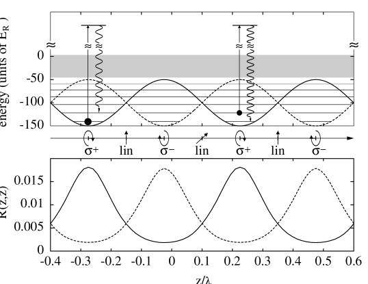
Figure 7: In the upper panel the optical bipotentials and bandstructure of the atom are plotted as a function of position $z$ for a $1/2$ to $3/2$ transition. The potential depth is $U_{0}=100E_{R}$. The excited states were adiabatically eliminated. We schematically indicate the two Raman processes between the ground and excited states which lead to the red and blue sidebands in resonance fluorescence. In the lower panel we show the spatial distribution of the atoms in the $|g_{+}\rangle$–state (solid line) and $|g_{-}\rangle$–state (dashed line) for $U_{0}=100E_{R}$ and ${\gamma}_{0}=5/3E_{R}$. The atoms are localized in the valleys of the corresponding optical potentials [26].

where $\omega$ is the frequency, $k=2\pi/\lambda$ the wave vector with $\lambda$ the wavelength of the laser light, and $\mbox{$\bf e$}_{\pm 1}$ are spherical unit vectors. For red laser detunings $\Delta=\omega-\omega_{eg}$ and low laser intensities, i.e. small saturation parameter $s={\Omega^{2}/2/(\Delta^{2}+\Gamma^{2}/4)}<<1$ with $\Omega$ the Rabi frequency and $\Gamma$ the spontaneous decay width, the Stark shifts of the two $|g_{-}\rangle$ and $|g_{+}\rangle$ ground states will form an alternating pattern of optical bipotentials $U_{\pm}(z)$. This is shown in the upper part of Fig. 7: due to the large Clebsch–Gordan coefficients for the outer transitions (see Fig. 6), minima will occur for the state $|g_{\pm}\rangle$ at positions with pure $\sigma^{\pm}$–light. In addition, spontaneous emission causes transitions between these potentials via optical pumping processes. In the semiclassical picture of Sisyphus–cooling [57] one considers an atom moving on one of these potential curves, say $U_{-}(z)$. Transitions to the other potential $U_{+}(z)$ then occur preferentially from the tops of $U_{-}(z)$ down to the valleys of $U_{+}(z)$, so that on the average the atomic motion is damped. Quantum mechanically, laser cooling can be understood as optical pumping between the quantized energy levels (band structure) in the limit of level separations $\hbar\omega_{\rm osc}$ much larger than the optical pumping rate $\gamma_{0}=s\Gamma$ (which implies large laser detunings) [56]. In the time domain this condition corresponds to a situation in which an atomic center-of-mass wave packet in the potential undergoes many oscillations with frequency $\omega_{\rm osc}$ before an optical pumping process occurs [26]. An example of a band structure is shown in the upper part of Fig. 7. As a result of laser cooling the atom will occupy the lowest energy levels, and will thus be strongly localized. The lower part of 7 shows the corresponding localization of the atom in minima of the $U_{\pm}(z)$ potentials. Transitions between the vibrational states will manifest themselves as sidebands (Raman transitions due to optical pumping) in the atomic absorption and emission spectra [52, 53, 54].

The basis of a theoretical discussion of laser cooling is the solution of the Generalized Optical Bloch Equations for the atomic density matrix comprising both the internal and external (center–of–mass) degrees of freedom [55]. The corresponding master equation for the density matrix $\rho$ of the ground state manifold and 1D motion in the $z$–direction is [26, 56] ($\hbar=1$)

$$\dot{\rho}= - i({H_{\rm eff}}(\hat{z})\rho-\rho{H_{\rm eff}}(\hat{z})^{\dagger})$$ (166)

$$+ \gamma_{0}\sum_{\sigma}\int_{-1}^{+1}du\;N_{\sigma}(u)B_{\sigma}(\hat{z})e^{-iku\hat{z}}\rho B_{\sigma}(\hat{z})^{\dagger}e^{iku\hat{z}}.$$

$N_{\sigma}(u)$ is the angular distribution of spontaneous photons emitted in the direction $u=\cos(\stackrel{{\scriptstyle\rightarrow}}{{k}}_{s},\stackrel{{\scriptstyle\rightarrow}}{{e}}_{z})$ with polarization $\sigma=0,\pm 1$, and $\gamma_{0}=s\Gamma/2$ is the photon scattering rate. The first two terms on the right-hand side of the master equation involve the non-Hermitian atomic Hamiltonian

$${H_{\rm eff}}(\hat{z})=\frac{\hat{p}^{2}}{2M}-(U_{0}+i\frac{1}{2}\gamma_{0})\sum_{\sigma}B_{\sigma}(\hat{z})^{\dagger}B_{\sigma}(\hat{z})$$ (167)

describing the motion of the atomic wavepacket with kinetic energy $\hat{p}^{2}/2M$ in a multicomponent optical potential with depths determined by $U_{0}={s|\Delta|/2}$. The real part of the potential in (167) gives rise to quantized energy levels (band structure), while the imaginary part describes a loss rate due to optical pumping. The operators $B_{\sigma}(z)$ correspond to Raman transitions between the ground state levels by absorption of a laser photon and subsequent emission of a spontaneous photon with polarization $\sigma$, see Ref.[26]. The master equation (166) is of the Lindblad form with an infinite number of channels (the $u$ integration over the $z$–projection of the emitted photon wave vector in Eq. (166))

We are interested in the spectrum of resonance fluorescence, emitted along the $z$-axis, with frequency $\omega^{\prime}$ and polarization $\sigma$. This spectrum is proportional to the Fourier transform of the stationary atomic dipole correlation function [26]

$$c_{\sigma}(t-t_{0})=\langle B_{\sigma}(t)^{\dagger}\;e^{ik^{\prime}_{z}\hat{z}(t)}\;B_{\sigma}(t_{0})\;e^{-ik^{\prime}_{z}\hat{z}(t_{0})}\rangle\;.$$ (168)

According to Section 0.4.4 and Ref.  [26] we have

$$c_{\sigma}(t-t_{0})={\rm Tr}_{S}\left\{B^{\dagger}_{\sigma}\;e^{ik_{z}\hat{z}}\;\rho^{(+)}(t)\right\}\quad(t\geq t_{0})\;\;\;;$$ (169)

where the first order perturbed density operator $\rho^{(+)}(t)$ obeys the same master equation as the density matrix but with a different initial condition

$$\rho^{(+)}(t_{0})=B_{\sigma}(\hat{z})\;e^{-ik^{\prime}_{z}\hat{z}}\rho(t_{0})\;.$$ (170)

Physically, this simulation procedure can be interpreted as the following computer experiment [14, 21, 26] (for a more formal derivation see Sec. 0.4.4). We surround the atom by an (infinite number of) unit efficiency photodetectors covering the $4\pi$ solid angle. The simulated “click” of the photodetectors determines the time, polarization and direction of the emitted photon (see Fig. 5 a). This is the simulation of the density matrix of the laser cooled atom. To simulate the fluorescence spectrum, we place a Fabry-Perot in front of one of these photodetectors and “measure” the transmitted photon flux. This gives the spectrum as a function of the tuning of the resonance frequency of the Fabry-Perot transmission (see Fig. 5 b).

In the experiment by Jessen et al.  the resonance fluorescence spectrum from Rb⁸⁵ atoms in 1D molasses is observed. The Rb atoms are driven on the $5S_{1/2}$ $F_{g}=3\rightarrow 5P_{3/2}$ $F_{e}=4$ transition in a lin $\perp$ lin laser configuration described above. In this case a direct solution of the master equation (166) to calculate the autocorrelation function (169) is impractical due to the large dimensionality of the density matrix equation which involves $N^{2}$ elements ($N=N_{ex}\times N_{\rm int}$ where $N_{int}$ is the number of internal, and $N_{ex}$ the number of (discretized) external degrees of freedom). For ⁸⁵Rb we have $N=448$ on a Fourier grid with 64 points corresponding to momenta up to $\pm 32\hbar k$ [26]; $10000$ wavefunction realizations are needed for convergence.

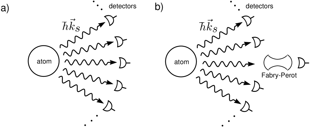
Figure 5: (a) The “experiment” simulated in the Monte Carlo wave function description of optical molasses: the atom is surrounded by photo detectors corresponding to an angle resolved detection of the emitted photon $\hbar\stackrel{{\scriptstyle\rightarrow}}{{k}}_{s}$. (b) Simulation of the fluorescence spectrum of the emitted light: the atom is “observed” with photodetectors and the spectrum is obtained by filtering one output channel with a Fabry-Perot interferometer [26].

Adapting the formalism of Sec. 0.4.3 a simulation of the master equation (166) consists of propagation of an atomic wave function ${\tilde{\psi}}_{c}(t)$ with the non–Hermitian (damped) atomic Hamiltonian (167) interrupted at random times by wave function collapses

$${{{{\tilde{\psi}}_{c}(t\!+\!dt)}}}=e^{ik^{\prime}_{z}\hat{z}}B_{\sigma}(\hat{z}){{{{\tilde{\psi}}_{c}(t)}}},$$ (171)

and subsequent wave function renormalization. The Schrödinger equation for ${{{{\tilde{\psi}}_{c}(t)}}}$ describes the time evolution of the atomic wave packet in the periodic optical potential, and its coupling to the laser driven internal atomic dynamics. The times of the “quantum jumps” are selected according to the delay function

$$\tilde{c}(u^{\prime},\sigma,t)=|\!|\sqrt{\gamma_{0}\;N_{\sigma}(u^{\prime})}\;B_{\sigma}(\hat{z}){\tilde{\psi}}_{c}(t)|\!|^{2}$$ (172)

which gives the probability for emitting a spontaneous photon at time $t$, with momentum $k^{\prime}_{z}=ku^{\prime}$ along the z-axis and polarization $\sigma$. The “quantum jump” (171) corresponds to an optical pumping process between the atomic ground states, including the associated momentum transfer to the atom. Averaging over these wave function realizations gives the density matrix according to Eq. (121).

The dipole correlation function (169) can be simulated following the approach outlined in section 0.4.4 [14, 21, 26]. The perturbed density matrix $\rho^{(+)}(t)$ in Eq. (169) can be interpreted as a first order response to a “delta-kick” at time $t=t_{0}$, represented by the initial condition (170,132). A simulation is obtained by introducing a “perturbed” wave function ${{{{\tilde{\psi}}_{c}^{(+)}(t)}}}$ which obeys the Schrödinger equation for ${{{{\tilde{\psi}}_{c}(t)}}}$ but now with initial condition [compare Eq.(170,132)]

$${{{{\tilde{\psi}}_{c}^{(+)}(t=t_{0})}}}=e^{-ik^{\prime}_{z}\hat{z}}B_{\sigma}(\hat{z}){{{{\tilde{\psi}}_{c}(t_{0})}}},$$ (173)

and quantum jumps of ${{{{\tilde{\psi}}_{c}^{(+)}(t)}}}$ dictated by the wave function ${{{{\tilde{\psi}}_{c}(t)}}}$ according to the delay function (172). The dipole correlation function is

$$c_{\sigma}(t-t_{0})=\left\langle\langle{{\tilde{\psi}}_{c}(t)}|B_{\sigma}(\hat{z})^{\dagger}e^{ik^{\prime}_{z}\hat{z}}{|{{\tilde{\psi}}_{c}^{(+)}(t)}\rangle}/|\!|{\tilde{\psi}}_{c}(t)|\!|^{2}\right\rangle_{\rm st}$$ (174)

where the angular brackets indicate averaging over both quantum jumps and initial times $t_{0}$.

The periodicity of the atomic Hamiltonian (167) in space, and assuming an infinite periodic molasses, allows one to propagate the atomic wave packets as time dependent Bloch functions

$${\tilde{\psi}}_{c}(z,t)={1\over\sqrt{2\pi}}\;e^{iqz}u_{q}(z,t)$$ (175)

with $q\in(-k,k]$ a quasi momentum in the first Brillouin zone, and $u_{q}(z,t)=u_{q}(z+\lambda/2,t)$ a periodic multicomponent atomic wave function. The Hamiltonian evolution due to $H_{\rm eff}$ preserves $q$, while quantum jumps cause changes between families of Bloch functions, $q\rightarrow q^{\prime}$. In practice, we propagate the Bloch function $u_{q}(z,t)$ on the unit cell of the lattice $z\in[0,\lambda)$ using a split-operator Fast-Fourier Transform method [26].

Figure 8 compares the resonance fluorescence spectrum for $\sigma^{+}$ polarized light obtained by simulation (solid line) with the experimental data of Jessen et al. [52] (crosses) for laser intensities, detunings etc. taken directly from the experiment with no adjustable parameter. The theoretical spectrum of Fig. 8 was obtained by convolving the ab initio spectrum with the experimental resolution. The central line is scattering at the laser frequency while the first red and blue sidebands correspond to Raman transitions between adjacent vibrational bands in the optical potential. The asymmetry of the red and blue sideband intensities reflects the populations of the vibrational levels, and from the excellent agreement between theory and experiment we infer that the wave function simulation reproduces the experimental temperature of the atoms[52]. Laser cooling accumulates atoms predominantly in the lowest vibrational states and in the $M_{g}=\pm 3$ potentials. This spatial localization of atoms – on a scale small compared with the laser wavelength – suppresses optical pumping transitions between different vibrational levels $n\neq n^{\prime}$, which is responsible for a narrowing of the lines in the optical spectrum (Lamb–Dicke narrowing). A broadening mechanism is present for the sidebands, due to the anharmonicity of the optical potential. This leads to different transition frequencies for $n\rightarrow n\pm 1$ (by approx. $E_{R}/\hbar$). For the present parameters this anharmonicity is not resolved even in the unconvolved spectrum.

Figure 6: Atomic level scheme and Clebsch-Gordan coefficients for a $J_{g}=1/2$ to $J_{e}=3/2$ transition in a lin $\perp$ lin configuration [26].

Figure 8: Spectrum of resonance fluorescence as a function of the frequency $\nu$. The solid line is the theoretical spectrum [26] convolved with a Lorentzian corresponding to a finite detector width of $3.8$ kHz and a Gaussian with width $20$ kHz (residual Doppler broadening). Crosses are the experimental result of Jessen et al. [52]. The inset shows the total spectrum. For parameters we refer to Ref. [26].

Localization by Spontaneous Emission

As outlined in the context of Eq. (122) there is no unique way of decomposing a given master equation (58) to form quantum trajectories ${\tilde{\psi}}_{c}(t)$, since the reservoir measurement may be performed in any basis. This statement is equivalent to noting that Eq. (58) is form invariant under the substitution (122). Different sets of jump operators $\{{c}_{j}\}$ not only lead to a different physical interpretation of trajectories, but an appropriate choice of ${c}_{j}$ may be crucial for the formulation of an efficient simulation method for estimating the ensemble distribution [43]. We will illustrate these ideas in the context of the quantized motion of an atom moving in optical molasses for the master equation (166).

Simulation methods for modeling spontaneous emission according to the master equation (166) have assumed an angle resolved detection of the photon as illustrated in Fig. 1(a). For a one dimensional system with adiabatically eliminated excited state this gave the jump operators (171),

$$c_{u\sigma}=\sqrt{\gamma_{0}\,N_{\sigma}(u)}\,e^{-iku\hat{z}}B_{\sigma}(\hat{z})\quad\mbox{($-1\leq u\leq+1$, $\sigma=0,\pm 1$ )}\;.$$ (176)

In a simulation each quantum jump gives information on the direction of the emitted photon. Alternatively, we could observe the fluorescence through a lens (Fig. 9(b)). The wave function simulation in this case is equivalent to the direct simulation of a Heisenberg microscope [58]: it is not possible to distinguish different paths $u_{1}$ and $u_{2}$ (Fig. 9(b)) which may be taken by the photon so the decay operator does not generate a unique recoil. Instead, information about the position coordinate is provided by each emission event, and as a result the wavefunction is localized in position space. Applying a Fourier transform to the operators in Eq. (176) to model the action of the ideal lens gives the new decay operators for one dimension

$$c_{\nu\sigma}=\int_{-1}^{1}du\,\sqrt{\gamma_{0}N_{\sigma}(u)}B_{\sigma}(\hat{z})e^{-iku(\hat{x}-\nu\lambda/2)}\quad\mbox{($\nu=0,\pm 1,\ldots$)}\;.$$ (177)

For angle resolved detection, $u$ labels a continuous but bounded set of operators, so that in the conjugate basis, $\nu$ can be any integer and indexes an infinite set of operators at discrete points. The integral can be evaluated for $\hat{c}_{\nu=0\,\sigma}$ to give a localized function centered at the origin and the rest generated by translation by multiples of $\pm\lambda/2$. To prove that both sets of jumps operators (176) and (177) give rise to the same a priori dynamics, we consider the following identity for the recycling term in Eq. (166),

$${\cal J} {}_{\sigma}\rho\propto\int\limits_{-1}^{1}du\,\left(\sqrt{N_{\sigma}(u)}B_{\sigma}e^{iku\hat{z}}\right)\rho\left(\sqrt{N_{\sigma}(u)}B_{\sigma}e^{iku\hat{z}}\right)^{\dagger}=$$

$$= \sum\limits_{\nu=-\infty}^{\infty}\left(\int\limits_{-1}^{1}du\,\sqrt{N_{\sigma}(u)\over 2}B_{\sigma}e^{iku(\hat{z}-\nu\lambda/2)}\right)\rho\left(\int\limits_{-1}^{1}du^{\prime}\,\sqrt{N_{\sigma}(u^{\prime})\over 2}B_{\sigma}e^{iku^{\prime}(\hat{z}-\nu\lambda/2)}\right)^{\dagger}$$

where we have used

$$\delta(u-u^{\prime})=\frac{1}{2}\sum\limits_{\nu=-\infty}^{\infty}e^{i\pi\nu(u-u^{\prime})}\quad\mbox{($-1<u,u^{\prime}<+1$)}\;.$$ (179)

As an application of the new simulation method, we consider a fully quantum mechanical treatment of atomic diffusion in optical molasses for the lin $\perp$ lin laser configuration described above [43]. The calculation of quantum diffusion using the angle resolved detection approach is difficult because the wave function spreads out during the coherent propagation. In contrast to a description of an infinitely extended periodic molasses [26], we have here an intrinsically non-periodic problem. Applying the localizing jump operators (177) allows us to make use of a greatly reduced basis set which we allocate dynamically to follow the atom. One representative trajectory illustrating the random walks is shown in Fig. 10(a) where we plot the expectation value of the spatial coordinate as a function of time. The long periods when the position does not change appreciably correspond to sub-barrier motion when the total energy of the atom is below the threshold given by the maximum of the optical potential. Energy fluctuations allow eventually the atom to overcome the potential barrier as indicated by the dashed line in Fig. 10(b). It may then travel over several wavelengths until it is trapped again. For a more complete discussion of the spatial diffusion coefficient we refer to Ref. [43]. Other candidates for application of this method are cold collisions [59].

Figure 9: Schematic illustration of the two different measurement bases for the detection of spontaneous emission [43].

Figure 10: (a) Expectation value of the spatial coordinate for a single trajectory versus time. (b) Corresponding (kinetic plus potential) energy expectation value. Note the coincidences between above barrier energies and long flight periods over many wavelengths [43].

0.5.3 Quantum Computing, Quantum Noise and Continuous Observation

Quantum computers (QCs) (for a review see [60]) promise exponential speedup for certain classes of computational problems [61] at the expense of exponential sensitivity to noise [62, 63, 64, 65]. Thus the analysis and suppression of quantum noise is a fundamental aspect of any discussion of the practicality of quantum computing. The theory of quantum noise and continuous measurement discussed in the preceding sections provides the theoretical basis for such an analysis.

Computation is a process which transforms an initial state to a final state by the application of certain rules. These input and output states are represented by physical objects, and computation is the physical process which produces the final from the initial state. Quantum computers are physical devices which obey the laws of quantum mechanics, in the sense that the states of the computer are state vectors in a Hilbert space, and the processes are the unitary dynamics generated by the Schrödinger equation on this Hilbert space. The distinctive feature of QCs is that they can follow a superposition of computational paths simultaneously and produce a final state depending on the interference of these paths [60]. Recent results in quantum complexity theory, and the development of some algorithms indicate that quantum computers can solve certain problems efficiently which are considered intractable on classical Turing machines. The most striking example is the problem of factorization of large composite numbers into prime factors [61], a problem which is the basis of the security of many classical key cryptosystems: to factor a number $N$ of $L$ digits on a classical computer requires a time approximately proportional to $\exp L^{1/3}$ for the best known algorithms, while Shor has shown that for a QC the execution time grows only as a polynomial function $L^{2}$ [61].

Realization of the elements of a quantum computer

The basic elements of the QC are the quantum bits or qubits [60]. In a classical computer a bit can be in a state $0$ or $1$, while quantum mechanically a qubit can be in a superposition state $|\psi\rangle=c_{0}|0\rangle+c_{1}|1\rangle$ with $|0\rangle$ and $|1\rangle$ two orthogonal basis states in a two-dimensional state space ${\cal H}_{2}$. Quantum registers are defined as product states of $L$ qubits,

$$|\underline{x}\rangle=|x_{L-1}\rangle_{L-1}\ldots|x_{0}\rangle_{0}\in{\cal H}_{2}\otimes\ldots{\cal H}_{2}$$ (180)

with and $x_{n}=0,1$, and $x=\sum_{n=0}^{L-1}x_{n}2^{n}$ the binary decomposition of the number $x$. There are $2^{L}$ different states and the most general state of a quantum register is the superposition

$$|\psi\rangle=\sum_{\underline{x}=\{0,1\}^{L}}c_{\underline{x}}|\underline{x}\rangle\;.$$ (181)

In a QC the physical objects are state vectors $\Psi$ in the product space (181), and the computation is the Schrödinger time evolution ${\psi_{\rm in}}\rightarrow{\psi_{\rm out}}={\hat{U}}{\psi_{\rm in}}$ with ${\hat{U}}$ a unitary time evolution operator. Note that unitarity of ${\hat{U}}$ implies that the computation is reversible.

Physical problems in realizing a QC are:

• A physical realization for the qubits must be found. Examples are internal states of atoms, or photon number states or polarization states of photons.

• We must be able to erase the content of the register and to prepare the initial superposition state $\psi_{\rm in}$.

• The unitary evolution operator ${\hat{U}}$ must be implemented. The unitary transformation can be decomposed into a sequence of steps involving the conditional dynamics of a few qubits (quantum gates) [60].

  In particular, it has been shown that any operation can be decomposed into controlled–NOT gates between two qubits and rotations on a single qubit, where a controlled–NOT is defined by

  $$\hat{C}_{12}:|\epsilon_{1}\rangle|\epsilon_{2}\rangle\rightarrow|\epsilon_{1}\rangle|\epsilon_{1}\oplus\epsilon_{2}\rangle\quad\mbox{$\epsilon_{1,2}=0,1$}$$ (182)

  where $\oplus$ denotes addition modulo $2$. The question then is to find physical processes (i.e. a Hamiltonian) which implement these quantum gates.

• To read the state of the register $\psi_{\rm out}$ at the end of the computation we must implement and perform a von Neumann state measurement. These measurements are destructive, i.e. irreversible.

• In practice the central obstacle to building a QC is the fragility of macroscopic superpositions with respect to decoherence due to coupling of the QC to the environment, and the inaccuracy inherent to state measurements [62, 63, 64, 65]. Schemes and experimental realizations must be found which minimize these sources of decoherence.

Realization of quantum gates has been discussed in Refs. [50, 66, 67, 68, 69]. Cirac and Zoller [70] have proposed the implementation of a QC using laser cooled ions in a linear ion trap. The qubits are stored on a metastable atomic transition, while the ions undergo collective quantized motion in the linear trap [71], and interact individually with laser light. Exchange of phonons stimulated by laser pulses allows the implementation of quantum gates. The distinctive features of this system are: it allows the realization of quantum gates between any set of (not necessarily neighboring) ions; in comparison with other systems, decoherence is small, and the final readout of the output state can be performed with essentially unit efficiency employing the methods of quantum jumps. A first experimental implementation for quantum gates along these lines has been reported from the NIST Boulder group [72]. A QC based on optical CQED has been proposed by Pellizzari et al.  [73]. It is based on a string of atoms trapped inside a high Q optical cavity. Long lived Zeeman coherences of ground state atoms represent the qubits. Quantum gates between atoms are realized via exchange of a photon through the single quantized cavity mode [73]. As in the case of ion traps, quantum gates can be performed between any two qubits. Sources of incoherence in this model are cavity decay and spontaneous emission of atoms from the excited state during the gate operation. However, spontaneous emission can be significantly avoided by performing the gate operation between two atoms as an adiabatic passage process via a dark state of the strongly coupled atom+cavity system [74]; and cavity decay is minimized by having a photon present only during the gate operation.

Errors and their correction

There are two sources of errors in quantum computing. First, there are systematic errors, for example, due to uncertainties in adjustment of parameters. Second, there is decoherence as a result of coupling to the environment [62, 63, 64, 65]. The general state of a register of a QC is described by a density matrix

$$\rho(t)=\sum_{x,=0}^{2^{L}-1}\sum_{x^{\prime}=0}^{2^{L}-1}|x\rangle\rho_{x,x^{\prime}}(t)\langle x^{\prime}|\;.$$ (183)

Thus as a result of the contact with the environment there will be changes in populations (the diagonal density matrix elements), and decay of the coherences (the off-diagonal density elements) on a time scale determined by the coupling of the QC to the environment. The power of quantum computing results from interference between quantum paths, consequently a loss of coherence will destroy the quantum parallelism. Unruh [62] has shown that the computer–environment coupling leads to an exponential error rate with the number of qubits $L$, and it has been argued that this dependence will be the decisive factor to limit the size of problems which can be solved on the QC. What these limits are will be determined by fundamental limits of specific theoretical proposals for the decay of qubits and noise in quantum gates, and by technological and experimental progress. Specific models for dissipation have been studied in references [62, 63, 64, 65].

The above discussion of decoherence assumes that the environment is traced out, i.e. in the language of continuous measurement theory “the results of the measurements in the out channels are not read.” This is the situation where the time evolution of the density matrix (183) is described by the master equation (a priori dynamics). It is of interest to study the evolution of a QC which is continuously monitored to detect the decay (quantum jump), and thus an incoherent step in the evolution (compare nonlinear evolution Eq. (103, and the quantum jump described by Eq. (105) [73]. After detection of a decay the computer can be restarted; on the other hand, by restricting the ensemble to those computer runs with no decay, we improve the statistics for the read out. In the CQED example given above this could be a cavity decay, or a photon from a spontaneous emission of one of the atoms representing the qubits. Note, however, that - even when no decay is detected in a specific run - information is gained by this “non-observation of a decay” and this leads to a distortion of the superposition of the qubits. To illustrate the effects of damping and continuous observation, we consider the following simple example. Let us assume that we store a superposition (qubit) $|\psi(t\!=\!0)\rangle=c_{0}|0\rangle+c_{1}|1\rangle$ on an atomic transition with ground state $|0\rangle$ and excited state $|1\rangle$, where the upper state decays with a radiative rate $\Gamma$. At time $t\!=\!0$ we prepare the qubit in the superposition $|\psi(t\!=\!0)\rangle=c_{0}|0\rangle+c_{1}|1\rangle$. If we do not monitor the decay of the qubit (a priori dynamics), the time evolution of the qubit is governed by the solution of the master equation:

$$|\psi ( t\!=\!0)\rangle\langle\psi(t\!=\!0)|\rightarrow\exp{\cal L}t\,|\psi(0)\rangle\langle\psi(0)|$$

$$= |c_{0}|^{2}|0\rangle\langle 0|\left(1-e^{-\Gamma t}\right)+|c_{1}|^{2}|1\rangle\langle 1|e^{-\Gamma t}+\left(c_{1}c_{0}^{*}|1\rangle\langle 0|+{\rm H.c.}\right)e^{-\frac{1}{2}\Gamma t}\;.$$

We note that the initial pure state develops into a mixture, until the atom finally has decayed to the ground state. If we monitor the system continuously (with unit detection efficiency) and observe no decay (a posteriori dynamics), the state evolves according to (103) and remains a pure state; however the superposition is distorted by the decay (see also Ref. [19]):

$$|\psi(t\!=\!0)\rangle \rightarrow |\psi(t)\rangle=e^{-iH_{\rm eff}t}|\psi(0)\rangle/|\!|e^{-iH_{\rm eff}t}|\psi(0)\rangle|\!|$$

$$= \left(c_{0}|0\rangle+c_{1}|1\rangle e^{-\frac{1}{2}\Gamma t}\right)/|\!|\ldots|\!|$$

$$\rightarrow |0\rangle\quad\mbox{for $t\rightarrow\infty$}\;.$$

This unwanted dynamics of the qubits corresponds to our increase of information which we gain by observing (measuring) the system: by not registering a decay our knowledge increases that the system is in the ground state. The distortion of the qubit is a result of the asymmetry of the decay. When we flip the qubit at time $t/2$, $|0\rangle\leftrightarrow|1\rangle$ , and again at time $t$, we symmetrize the decay,

$$|\psi(t\!=\!0)\rangle \rightarrow \left(c_{0}|0\rangle e^{-\frac{1}{4}\Gamma t}+c_{1}|1\rangle e^{-\frac{1}{4}\Gamma t}\right)/|\!|\ldots|\!|$$

$$= c_{0}|0\rangle+c_{1}|1\rangle\equiv|\psi(t\!=\!0)\rangle\;.$$

Thus, the information which state has decayed has been lost, the superposition remains unchanged, and there is no effect of decay (in the subensemble with no decay). The idea of a symmetric decay, which factors out in the time evolution (103) and thus drops out upon normalization, is readily generalized to a construction of gates. This problem is studied in more detail in Ref. [73]. It is an interesting question to what extent schemes can be found where the state of the register can be reconstructed after a quantum jump [75].

Acknowledgment: We thank Klaus Ellinger, Simon Gardiner, Klaus Gheri, Thomas Pellizzari and Herwig Stecher for reading the manuscript. P.Z. thanks F. Haake for an exciting climb of Mont Blanc during the summer school.

.6 An exercise in Ito calculus

As an exercise in Ito calculus we will go in some detail through the steps of deriving Eq.(0.4.3) from (0.4.3). To simplify notation we confine ourselves to the case of a single channel ${N_{c}}=1$. We will show that if ${\tilde{\psi}}_{c}(t)$ obeys

$$d{\tilde{\psi}}_{c}(t)=[A\>dt+(B-\hat{1})dN{(t)}]{\tilde{\psi}}_{c}(t)$$ (187)

with $A$ and $B$ operators, then the normalized $\psi_{c}(t)$ obeys

$$d\psi_{c}(t)=[(A-\left\langle A+A^{\dagger}\right\rangle_{c})\>dt+(B/\sqrt{\left\langle B^{\dagger}B\right\rangle_{c}}-1)dN{(t)}]\psi_{c}(t)$$ (188)

with $\left\langle\ldots\right\rangle_{c}$ defined in Eq. (113).

Proof: From

$${\tilde{\psi}}_{c}(t\!+\!dt)=[\hat{1}+A\>dt+(B-\hat{1})dN{(t)}]{\tilde{\psi}}_{c}(t)$$ (189)

the change of the norm in the time step $dt$ is

$$|\!|{\tilde{\psi}}_{c}(t\!+\!dt)|\!|^{2}=|\!|{\tilde{\psi}}_{c}(t)|\!|^{2}\left[1+\left\langle A+A^{\dagger}\right\rangle_{c}\>dt+\left\langle B^{\dagger}B-\hat{1}\right\rangle_{c}dN{(t)}\right]$$ (190)

and

$$|\!|{\tilde{\psi}}_{c}(t\!+\!dt)|\!|^{-1} = |\!|{\tilde{\psi}}_{c}(t)|\!|^{-1}[1+\left\langle A+A^{\dagger}\right\rangle_{c}\>dt+\left\langle(B^{\dagger}B-\hat{1})\right\rangle_{c}dN{(t)}]^{-1/2}$$

$$= |\!|{\tilde{\psi}}_{c}(t)|\!|^{-1}[1-\frac{1}{2}\left\langle A+A^{\dagger}\right\rangle_{c}\>dt+(1/\sqrt{\left\langle B^{\dagger}B\right\rangle_{c}}-1)\;dN{(t)}]\;.$$

This follows from

$$f(1+a\>dt+b\;dN) = f(1)+f^{\prime}(1)\;a\>dt+f^{\prime}(1)\;b\;dN+\frac{1}{2!}f^{\prime\prime}(1)\;b^{2}\;dN^{2}+\ldots$$

$$= f(1)+f^{\prime}(1)\;a\>dt+[f(1+b)-f(1)]\;dN$$

valid for sufficiently well-behaved functions $f$. Finally, we have

$$\psi_{c}(t\!+\!dt) = [\hat{1}+A\>dt+(B-\hat{1})dN{(t)}]\psi_{c}(t)\times$$

$$[1-\frac{1}{2}\left\langle A+A^{\dagger}\right\rangle_{c}\>dt+(1/\sqrt{\left\langle B^{\dagger}B\right\rangle_{c}}-1)\;dN{(t)}]$$

which gives (188).

Bibliography

- [1]
- [2] C.W. Gardiner, Quantum Noise (Springer, Berlin, 1991).
- [3] H.J.Carmichael, An Open Systems Approach to Quantum Optics, Lectures Notes in Physics m18 (Springer, Berlin, 1993)
- [4] D.F. Walls and G. Milburn, Quantum Optics (Springer, Berlin, 1995).
- [5] W. Louisell, Quantum Statistical Theories of Radiation (Wiley, New York, 1974, 1989).
- [6] R. Hudson and K.R. Parthasarthy, Commun. Math. Phys. 93, 301 (1984).
- [7] C.W. Gardiner, Handbook of Stochastic Methods, 2nd Ed. (Springer, Berlin 1985, 1989).
- [8] A. Barchielli and G. Luperi, J. Math. Phys. 26, 1985 (1985).
- [9] A. Barchielli, Phys. Rev. A 34, 1642 (1986)
- [10] A. Barchielli, J. Phys. A 20, 6341 (1987).
- [11] A. Barchielli, Quantum Opt. 2, 423 (1990)
- [12] A. Barchielli and V. P. Belavkin, J. Phys. A 24, 1495 (1991) and references cited.
- [13] C.W. Gardiner and M.J. Collett, Phys. Rev. A 31, 3761 (1985).
- [14] C. W. Gardiner, A. S. Parkins, and P. Zoller, Phys. Rev. A 46, 4363 (1992).
- [15] H. M. Wiseman, Quantum Trajectories and Feedback, PhD Thesis, University of Queensland, June 1994; H. M. Wiseman and G. Milburn, Phys. Rev. A 47, 642 (1993); ibid. 1652 (1993).
- [16] M.D. Srinivas and E.B. Davies, Optica Acta 28, 981 (1981).
- [17] P. Goetsch and R. Graham, Phys. Rev. A 50, 5242 (1994); P. Goetsch, R. Graham and F. Haake, Phys. Rev. A 51 136 (1995).
- [18] J. Dalibard, Y. Castin, and K. Mølmer, Phys. Rev. Lett. 68, 580 (1992).
- [19] K. Mølmer, Y. Castin and J. Dalibard, J. Opt. Soc. Am. B, 10, 524 (1993).
- [20] R. Dum, P. Zoller, and H. Ritsch, Phys. Rev. A 45, 4879 (1992).
- [21] R. Dum, A.S. Parkins, P. Zoller, and C.W. Gardiner, Phys. Rev. A 45, 4879 (1992).
- [22] L. Tian and H. Carmichael, Phys. Rev. A 46, R6801 (1992).
- [23] M Naraschewski and A. Schenzle, Z. Phys. D 33, 79 (1995)
- [24] V. P. Belavkin, J. Phys. A. 22, L1109 (1989); V. P. Belavkin, J. Math. Phys. 31, 2930 (1990); V. P. Belavkin and P. Staszewski, Phys. Rev. A 45, 1347 (1992)
- [25] C. Cohen-Tannoudji, F. Bardou, and A. Aspect, in Laser Spectroscopy X, edited by M. Ducloy, E. Giacobino, and G. Camy (World Scientific, 1992).
- [26] P. Marte, R. Dum, R. Taieb, P. D. Lett and P. Zoller, Phys. Rev. Lett. 71, 1335 (1993); P. Marte, R. Dum, R. Taieb and P. Zoller, Phys. Rev. A 47, 1378 (1993).
- [27] R. Dum, P. Marte, T. Pellizzari and P. Zoller , , Phys Rev. Lett. 73, 523 (1994).
- [28] Y. Castin, K. Berg-Sorensen, J. Dalibard, K. Molmer, Phys. Rev. A 50, 5092 (1994)
- [29] G. Nienhuis, J. de Kloe, and P. van der Straten, JOSA B 12, 520 (1995)
- [30] Y. Castin, and K. Molmer, Phys. Rev. Lett. 74, 3772 (1995)
- [31] J. Steinbach, B. M. Garraway, and P. L. Knight, Phys. Rev. A 50, 3302 (1995)
- [32] B. M. Garraway, and P. L. Knight, Phys. Rev. A 50, 2548 (1994)
- [33] B. M. Garraway, and P. L. Knight, Phys. Rev. A 49, 1266 (1994)
- [34] H. J. Carmichael, Phys. Rev. Lett. 70, 2273 (1993) ; C. W. Gardiner, Phys. Rev. Lett. 70, 2269 (1993)
- [35] N. Gisin, Phys. Rev. Lett. 52, 1657 (1984); N. Gisin, Helv. Phys. Acta 62, 363 (1989).
- [36] N. Gisin and I.C. Percival, Phys. Lett. A 167, 315 (1992); J. Phys. A 25, 5677 (1992); J. Phys. A 26, 2233 (1993); N. Gisin, P. L. Knight, I. C. Percival, R. C. Thompson and D. C. Wilson, J. Mod. Opt. 40, 1663 (1993); N. Gisin,J. Mod. Opt. 40, 2313 (1993); Y. Salama and N. Gisin, Phys. Lett. A 181, 269 (1993).
- [37] S. Stenholm, Physica Scripta 47, 724 (1993).
- [38] L. Diosi, N. Gisin, J. Halliwell, and I. C. Percival, Phys. Rev. Lett. 74, 203 (1995)
- [39] P. Zoller, M. Marte and D. F. Walls, Phys. Rev. A 35 (1987); R. Blatt, W. Ertmer, J. Hall and P. Zoller, Phys. Rev. A 34, 3022 (1986).
- [40] B.R. Mollow, Phys. Rev. A 12, 1919 (1975).
- [41] R. Blatt and P. Zoller, Europ. J. Phys. 9, 250 (1988); R. J. Cook, Prog. Opt., 28, 361 (1990).
- [42] W. Nagourney, J. Sandberg, H. Dehmelt, Phys. Rev. Lett. 56, 2797 (1986); J. C. Bergquist, Randall G. Hulet, Wayne M. Itano, and D. J. Wineland, Phys. Rev. Lett. 57, 1699 (1986); Th. Sauter, W. Neuhauser, R. Blatt, and P. E. Toschek, Phys. Rev. Lett. 57 1696 (1986).
- [43] M. Holland, S. Marksteiner, P. Marte and P. Zoller, Phys. Rev. Lett. 76 3683 (1996).
- [44] See lecture notes by P. Knight, this volume.
- [45] H. Walther, Adv. in At. Mol. and Opt. Phys., 32, 379 (1994).
- [46] R. Blatt, Proc. 14-th ICAP, ed. S. Smith, C. Wieman, and D. Wineland et al. (AIP Press, 1995), p. 219.
- [47] C. Cohen–Tannoudji and J. Dalibard, Europhys. Lett. 1, 441 (1986).
- [48] J. I. Cirac, R. Blatt, A. S. Parkins and P. Zoller, Phys. Rev. Lett. 70, 762 (1993); J. I. Cirac, A. S. Parkins, R. Blatt and P. Zoller, Phys. Rev. Lett. 70, 556 (1993).
- [49] J. Eschner, B. Appasamy and P. E. Toschek, Phys. Rev. Lett. 74, 2435 (1995).
- [50] See lecture notes on CQED by J. M. Raimond, and S. Haroche, this volume.
- [51] K. Mølmer and Y. Castin, Quantum and Semiclass. Opt. 8 49 (1996) .
- [52] P.S. Jessen, C. Gerz, P. D. Lett, W. D. Phillips, S. L. Rolston, R. J. C. Spreeuw, C. I. Westbrook, Phys. Rev. Lett. 69, 49 (1992).
- [53] P. Verkerk, B. Lounis, C. Salomon, C. Cohen-Tannoudji, J. Y. Courtois and G. Grynberg, Phys. Rev. Lett. 68, 3861 (1992); G. Grynberg B. Lounis, P. Verkerk, J.-Y. Courtois, C. Salomon, Phys. Rev. Lett. 70, 2249 (1993).
- [54] A. Hemmerich and T. W. Hänsch, Phys. Rev. Lett. 70, 410 (1993).
- [55] H. Wallis, Physics Reports 255, 203 (1995).
- [56] Y. Castin and J. Dalibard, Europhys. Lett. 14, 761 (1991).
- [57] J. Dalibard and C. Cohen–Tannoudji, J. Opt. Soc. Am. B 6, 2023 (1989); J. Dalibard and C. Cohen-Tannoudji, J. Opt. Soc. Am. B 2, 1707 (1985).
- [58] T. Pfau, S. Spalter, Ch. Kurtsiefer, C. R. Ekstrom, J. Mlynek, Phys. Rev. Lett. 73, 1223 (1994).
- [59] M. J. Holland , K.-A. Suominen, and K. Burnett, Phys. Rev. Lett. 72, 2367 (1994).
- [60] For an review see, A. Ekert, Proc. 14-th ICAP, ed. S. Smith, C. Wieman and D. Wineland (AIP Press, 1995) p. 450.; R. Josza and A. Ekert, to appear in Rev. Mod. Phys.
- [61] P. Shor, Proc. 35-th Annual Symposium on Foundations of Computer Science, IEEE Press (1994).
- [62] W. G. Unruh, Phys. Rev. A 51, 992 (1995).
- [63] R. Landauer, Proc. Royal Soc. London A 353 367 (1995).
- [64] I. Chuang, R. Laflamme, P. Shor, and W. Zurek, Science 270 1633 (1995).
- [65] G. M. Palma, K.A. Suominen, and A. Ekert, Proc. Royal Soc. London A 452 567 (1996).
- [66] A. Barenco, D. Deutsch, and A. Ekert, Phys. Rev. Lett. 74, 4083 (1995).
- [67] T. Sleator and H. Weinfurter, Phys. Rev. Lett. 74, 4087 (1995).
- [68] D. P. DiVincenzo Phys. Rev. A 51, 1015 (1995)
- [69] P. Domokos, J. M. Raimond, M. Brune, and S. Haroche, Phys. Rev. A 52 3554 (1995).
- [70] J. I. Cirac and P. Zoller, Phys. Rev. Lett. 74, 4091 (1995).
- [71] M. G. Raizen, J. M. Gilligan, J. C. Bergquist, W. M. Itano, and D. J. Wineland, Phys. Rev. A 45, 6493 (1992).
- [72] C. Monroe, D. M. Meekhof, B. E. King, W. M. Itano, and D. Wineland, Phys. Rev. Lett. 75 4714 (1995).
- [73] T. Pellizzari, S. A. Gardiner, J. I. Cirac, and P. Zoller, Phys. Rev. Lett. 75 3788 (1995).
- [74] A. S. Parkins, P. Marte, P. Zoller, and H. J. Kimble, Phys. Rev. Lett. 71, 3095 (1993).
- [75] P.Z. thanks A. Barenco and H. Mabuchi for discussion of these ideas during the school.