The Wave Function in Quantum Mechanics

Abstract

Through a new interpretation of Special Theory of Relativity and with a model given for physical space, we can find a way to understand the basic principles of Quantum Mechanics consistently from Classical Theory. It is supposed that natural phenomena have a connection with intangible reality which cannot be measured directly. Futhermore, the intangible reality is supposed as vacuum particles – vacuum electrons are chosen as a model, each of which has energy $E{\sim}-m_{e}{c^{2}}$ in Dirac sea. In addition, 4-dimensional complex space is introduced, in which each dimension has an internal complex space.

Key Words : intangible reality – vacuum particles.
4-dimensional complex space.
internal complex space.

1 Introduction

Although we don’t have to review whole philosophy behind physics, at least we need to mention the philosophical attitude on which this article is based. Since $19^{th}$ century positivism or empiricism has been a concrete, non-compatible philosophical background in natural science; however, in the view of realism Quantum philosophy – the Berkeley-Copenhagen interpretation – seems running to an extreme case of the philosophy.

On the other hand, the positivism – mainly based on phenomenological facts(materialism) – is the most clear way in discussion of natural science including phisics. But, its limitation also appears in discussion of fundamental physics [1][2][3][4][5].

To discuss the realism – based on truth(idealism) not on materialism – there is a good example, that is, Allegory of the Cave[6] by Socrates and written by Plato – philosophers in ancient Greek.

• The cave represents the sensible world, the prisoners are nonphilosophers, and their fire represents the sun. The upper world outside the cave represents the intelligible realm, the released prisoners are philosophers, and the sun represents the good.[7][8]

In the parable of the cave, the dwellers cannot recognize the truth – puppets themselves – but can perceive only shadows of the puppets. This is a metaphor which means the limitation of phenomenological facts in presenting truth. For instance, the dwellers – as positivists – can consider the shadows themselves as truth. Then, how often they might have to ask God to explain their unsolved problems?

In this respect, ontological review of fundamental physics is necessary, then some epistemological interpretation should be followed. The purpose of this article is not to make Quantum Mechanics little but to understand it comprehensively with Special Theory of Relativity because real problems do not go away but merely change their appearance.

In Quantum Mechanics, what is the physical entity represented by the wave function? and how can we understand one particle double slits experiment? Should we accept the wave function itself as a physical entity? If that is true, how can we understand wave function collapse from finite probability to absolute one in the measurement of physical quantity? Even though Quantum Mechanics is so useful to get some practical results, we might have overlooked something more fundamental.

In Special Theory of Relativity, how can we understand why the speed of light is constant to all inertial observers and where the increased energy(or mass) is comming from? However, according to the theory itself, the mass increase depends on only relativistic motion between two inertial frames regardless of their interaction.

With a model for physical space and light propagation, we find a way to understand the physical entity of the wave function in Quantum Mechanics. It is assumed that negative-energy-mass particles in Dirac sea be considered in physical interactions, and that physical space consist of 4-dimensional complex space, in another words, each dimension has real and imaginary parts.

In Section 2, without any Quantum Mechanical concept a universal constant is searched in Special Theory of Relativity itself. In Section 3, 4-dimensional complex space is suggested for physical space, and the relations between the real and imaginary space are assumed. With a model suggested in Section 3.1, light propagation mechanism and the physical meaning of photon are studied. In Section 4, the interpretation of inertial mass and physical momentum is searched, and then the physical entity of wave function in Quantum Mechanics and the relation with physical momentum are searched. In Section 5, Fundamental questions – wave function collapse, one-particle-double-slits experiment, and photoelectric effect – are discussed. Finally, conclusion follows at the end.

2 A universal constant for light

In Special Relativity, we know that the wave vector(${k_{o}}$, ${\vec{k}}$) of light and the momentum ($p_{o}$, ${\vec{p}}$) are Lorentz 4-vectors with null lengths because of phase invariance in the wave vector and energy-momentum conservation, respectively. In proper Lorentz transformation, we can find that the ratio of $k_{\mu}$ to $p_{\mu}$ in each componemt is Lorentz scalar, which is independent of Lorentz transformation as long as the momentum ${\vec{p}}$ is parallel to the wave vector ${\vec{k}}$. Although we already know that the constant is Plank’s constant($h$), with one assumption we can confirm the universal constant from Special Relativity itself without using any Quantum Mechanical concept.

Now let us think a light wave motion(electromagnetic wave) in free space and assume that the momentum($p_{\mu}$) and the wave vector($k_{\mu}$) are unique to describe the wave motion at least in the energy and momentum. Suppose that those two vectors are parallel to each other in their space components. If we can assume that ${\vec{p}}={\alpha}{\vec{k}}$ (${\alpha}$ : constant), it is so trivial; however, we cannot be sure if the ${\alpha}$ is a function of ${k_{o}}$, ${p_{o}}$ or both in the inertial frame.

Figure 1: Lorentz transformation with arbitrary ${\vec{\beta}}$

Fig.(1) represents a Lorentz transformation for an arbitrary velocity ${\vec{\beta}}$. Let us say, ${k_{\parallel}^{\prime}}$ is parallel component and ${k_{\bot}^{\prime}}$ is perpendicular component to the direction of ${\vec{\beta}}$ in ${O^{\prime}}$-frame. The relations in the Lorentz transformation are

$${k_{\parallel}^{\prime}}=k{\gamma}(\cos{\theta}-{\beta}),\makebox[14.22636pt]{}({\gamma}={1\over{\sqrt{1-{\beta}^{2}}}},\makebox[11.38109pt]{}{k=|{\vec{k}}|=k_{o}={\omega\over c}})\makebox[14.22636pt]{}$$

$${k_{\bot}^{\prime}}=k_{\bot},\makebox[244.69386pt]{}$$

$${k_{o}^{\prime}}=k_{o}{\gamma}(1-{\beta}{\cos{\theta}}),\makebox[113.81102pt]{}\makebox[71.13188pt]{}$$

in which ${\theta}$ is the direction of cosine angle between ${\vec{k}}$ and ${\vec{\beta}}$ in O-frame. Likewise, the momentum $p_{\mu}$ has to be the same functional form as the wave vector $k_{\mu}$, that is

$${p_{\parallel}^{\prime}}=p{\gamma}(\cos{\theta}-{\beta}),\makebox[14.22636pt]{}({\gamma}={1\over{\sqrt{1-{\beta}^{2}}}},\makebox[11.38109pt]{}{p=|{\vec{p}}|=p_{o}={E\over c}})\makebox[14.22636pt]{}$$

$${p_{\bot}^{\prime}}=p_{\bot},\makebox[244.69386pt]{}$$

$${p_{o}^{\prime}}=p_{o}{\gamma}(1-{\beta}{\cos{\theta}}).\makebox[113.81102pt]{}\makebox[71.13188pt]{}$$

For each parallel or perpendicular component in $(p_{o},\vec{p})$ and $(k_{o},\vec{k})$, the ratios of the momentum to the wave vector are

$${{p_{\parallel}^{\prime}}\over{k_{\parallel}^{\prime}}}\makebox[5.69054pt]{}=\makebox[5.69054pt]{}{p\over k}\makebox[5.69054pt]{}=\makebox[5.69054pt]{}{p_{\parallel}\over k_{\parallel}}\makebox[5.69054pt]{}\equiv\makebox[5.69054pt]{}{f_{\parallel}},\makebox[170.71652pt]{}$$

$${{p_{\bot}^{\prime}}\over{k_{\bot}^{\prime}}}\makebox[5.69054pt]{}=\makebox[5.69054pt]{}{p_{\bot}\over k_{\bot}}\makebox[5.69054pt]{}\equiv\makebox[5.69054pt]{}{f_{\bot}},\makebox[199.16928pt]{}$$

$${{p_{o}^{\prime}}\over{k_{o}^{\prime}}}\makebox[5.69054pt]{}=\makebox[5.69054pt]{}{p_{o}\over k_{o}}\makebox[5.69054pt]{}\equiv\makebox[5.69054pt]{}{f_{o}}.\makebox[210.55022pt]{}$$

Here, we defined $f_{\parallel}$, $f_{\bot}$, and $f_{o}$ – Lorentz scalars since the ratios are independent of $\vec{\beta}$ and $\theta$. In addition, we already know that $f_{\parallel}$ is same to $f_{o}$. Now let us choose a $\vec{\beta}^{\prime}$ to exchange $p_{\parallel}$ $\leftrightarrow$ $p_{\bot}$ and $k_{\parallel}$ $\leftrightarrow$ $k_{\bot}$ because the ratios are Lorentz scalars. Then we can conclude that $f_{\parallel}=f_{\bot}=f_{o}\equiv f$, that is

$${p_{\mu}\over k_{\mu}}=f\makebox[56.9055pt]{}\makebox[113.81102pt]{({$\mu$} = {\small 0,1,2,3 \/}}\makebox[71.13188pt]{in any inertial frame.)}$$

With the fact that $p{\lambda}({\lambda={2\pi\over k}})$ is a Lorentz scalar, let us suppose that there are two light waves with wave lengths, ${\lambda}_{1}$ and ${\lambda}_{2}$ in O-frame(Fig.1). If the amplitudes of the waves are same, then the energies($p_{o}$) are determined only by the wave lengths or the frequencies ($k={2\pi\over{\lambda}}$, $c={\nu}{\lambda}$) because there is no difference in these two waves – in classicsl point of view – as far as our concerning is focussed on the energy and momentum only. Now, let us suppose that ${{{\lambda}_{1}}^{\prime}}$ in $O^{\prime}$-frame became to – through a continuous Lorentz transformation – equal to the ${{\lambda}_{2}}$ in O-frame, then ${E_{1}}^{\prime}$ is equal to ${E_{2}}$ because we assumed the same amplitudes. Therefore, $p{\lambda}$ is not only Lorentz scalar but also a universal constant.

In above argument, we assumed same amplitudes for the light waves and thus confirmed a universal constant without quantum mechanical concept. But still we don’t know if there is a fundamental energy unit in $E=pc$ or not.

3 Vacuum Particles and Physical Space

3.1 Physical Vacuum

From Dirac’s hole theory[9][10], we already know the existence of negative energy mass particles in vacuum. Let us call those particles vacuum particles. In vacuum, all possible states are occupied with fermions of each kind, and an antiparticle, in real world, is a hole in vacuum; however, unfortunately physical vacuum itself has not been studied much. According to the theory we cannot directly measure the physical behavior of vacuum particles because it is not in real world. Only by using antiparticles, we can guess the vacuum particles behavior like a mirror image since we believe energy-momentum conservation and charge conservation at least. Let us define real world for physical phenomena, imaginary world for the intangible one and dual world for both the real and imaginary worlds.

In stationary vacuum, we can suppose that the electrons, for instance, are not packed completely, but that they have spatial gaps among them because we can describe a positron using a wave function in quantum mechanics. In other words, there must be some uncertainty(${\mit\Delta}{\vec{r}}>0$) for the position, which means that vacuum electrons also have to have that uncertainty in vacuum. In addition, vacuum polarization[11] is another clue for the spacial gaps. For stationary vacuum we can assume that the vacuum particles are bounded with negative energies, and that the change of their energy produced by any possible perturbation appears in real world because of energy conservation. Now, if vacuum particles have spacial gaps among them, their individual motions can be transfered to neighbors in vacuum. Therfore, we can imagine a string vibration for the vacuum particles, which the string consists of. In phenomena these vacuum particles(negative energy mass particles in vacuum) already have been included, but in measurements only real values have meaning in physics. Even though we concern only real values as the final results, we need to care about the interaction mechanism to understand the results with more fundamental way. For instance, how can we understand electron-positron pair creation and the annihilation without vacuum particles? In fact, the model(Dirac sea) itself is still argumentable among theorists, but at least we can accept the existence of vacuum particles and the interactions with real physical object.

Let us assume followings :

• Physical space-time consists of 4-dimensional complex space(Riemann). That is, each dimension has an internal complex space uniquely, in which any complex function is satisfied with Cauchy-Riemann conditions.

• In inertial frame, the real time inteval is the same with the imaginary time interval in absolute value.

• In real world, physical object is in real 3-D subspace with real time even though the object actually has complex coordinates (${\xi}_{x},{\xi}_{y},{\xi}_{z}$).

• In imaginary 3-D subspace with imaginary time, where vacuum particles reside, physics law is the same as the law in real world. But in measurements, only the change of real values is measured on real coordinates.

• There are spacial gaps among vacuum particles, and those particles are bounded with negative energy(${E\sim-m_{e}c^{2}}$) in the view from real world; however, all possible vacuum states are occupied by each kind of fermions, but let us consider just only stationary vacuum electrons as a model.

• Any change in imaginary world reflects to real world and vice versa.
  For instance, vacuum particles keep interacting with real physical object.

• Light propagation is made by the vacuum electron-string vibrations in transverse mode.
  The propagation is in the imaginary axis of an internal complex space.

According to the assumptions above, stationary vacuum electrons are occupied in 3-dimensional complex space and keep interacting with real physical object in real world. For instance, how can we understand electromagnetic interaction? Long time ago we explained the interaction with action at the distance, and then we became to know that actually photons propagate in the interaction. Is that reasonable enough to explain the field? How can the photons know the direction to propagate? Now we can find a possible explanation for that question: When a charged or gravitational object is introduced to physical space, vacuum particles are rearranged to be more stable; thus, we might say this is the physical entity of the field.

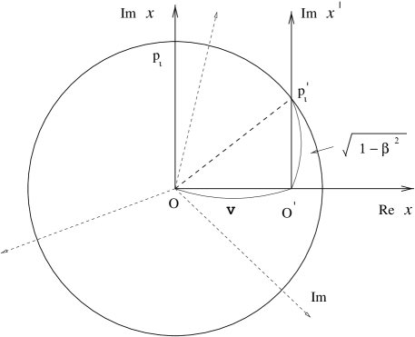
Figure 2: 3 dimensional complex space($\beta=v/c$)

3.2 Time Dilation and Length Cotraction

In Special Theory of Relativity, one of assumptions is about the speed of light in free space, which is the same for all inertial observers. Now we need to review this assumption with the physical space we are assuming. If the propagation of light follows the imaginary axis in an internal complex space – assumption(7), the speed of light is independent of a relativistic constant of motion on real axis because of the orthogonality between the real and imaginary axis. Since the time interval is same on the imaginary and the real axis of an inertial frame – assumption(2), the scales in both axises are also same, the wave front of light in the imaginary axis is corresponded to the real axis with the exactly same coordinate as the imaginary because the change of energy in vacuum is mapped to real world – assumption(6).

In Fig.(2), there are two observers – A at the origin and B with the velocity($v$) in $x$-direction. When the moving observer B passed through the origin, they sinchronized their watches to zero and a light source started radiating from the origin. One second later, the observer A at the origin of O-frame recognize that the moving observer’s time is $\sqrt{1-{\beta^{2}}}$ because the light signal in ${O^{\prime}}$-frame propagated from ${O^{\prime}}$ to ${{p_{i}}^{\prime}}$ through the imaginary ${x^{\prime}}$ axis and the time interval equals to the imaginary time interval in the internal complex space. However, this time dilation effect is the same to observer B since the effect is relativistic.

With a similar procedure as above we can also show the length contraction effect. Let us say, in O-frame a rod is appended at the origin and extended to $x=L_{o}$ – proper length. At $t=L_{o}/v$, the origin of ${O^{\prime}}$-frame is at $x=L_{o}$ and $t^{\prime}=(L_{o}/v)\sqrt{1-\beta^{2}}$. Definitely observer A, thus, surmise that observer B estimate the length of the rod as $L^{\prime}=L_{o}\sqrt{1-\beta^{2}}$.

3.3 Internal Complex Space

According to the assumptions of physical space, 3-dimensional complex vector is

$${\vec{\xi}}\makebox[2.84526pt]{}=\makebox[2.84526pt]{}\xi_{x}{\vec{i}}\makebox[2.84526pt]{}+\makebox[2.84526pt]{}\xi_{y}{\vec{j}}\makebox[2.84526pt]{}+\makebox[2.84526pt]{}\xi_{z}{\vec{k}},\makebox[28.45274pt]{}$$ (1)

$$\makebox[28.45274pt]{}=\makebox[2.84526pt]{}(x,y,z)\makebox[2.84526pt]{}+\makebox[2.84526pt]{}i(x_{i},y_{i},z_{i}).\makebox[28.45274pt]{}$$

In the expression, ${\vec{r}}=(x,y,z)$ and ${\vec{r}_{i}}=(x_{i},y_{i},z_{i})$ were used for the real and the imaginary coordinates, respectively. Then complex length element $d{\vec{l}}_{c}$ is defined as

$$d{\vec{\xi}}=(dx,dy,dz)\makebox[2.84526pt]{}+\makebox[2.84526pt]{}i(dx_{i},dy_{i},dz_{i}),$$

and the absolute length square is

$$l^{2}\makebox[2.84526pt]{}=\makebox[2.84526pt]{}{\vec{\xi}}\cdot{\vec{\xi}^{*}},\makebox[113.81102pt]{}$$

$$\makebox[28.45274pt]{}=\makebox[2.84526pt]{(}x^{2}+y^{2}+z^{2})\makebox[2.84526pt]{}+\makebox[2.84526pt]{}({x_{i}}^{2}+{y_{i}}^{2}+{z_{i}}^{2}).$$

Here, the real length, $r=\sqrt{x^{2}+y^{2}+z^{2}}$ and the imaginary length,
$r_{i}=\sqrt{{x_{i}}^{2}+{y_{i}}^{2}+{z_{i}}^{2}}$. So,

$$l\makebox[2.84526pt]{}=\sqrt{\makebox[2.84526pt]{}r^{2}\makebox[2.84526pt]{}+\makebox[2.84526pt]{}{r_{i}}^{2}},\makebox[85.35826pt]{}$$ (2)

and the complex length is

$$l_{c}\makebox[2.84526pt]{}=\makebox[2.84526pt]{}r\makebox[2.84526pt]{}+\makebox[2.84526pt]{}i\makebox[1.42262pt]{}r_{i}.\makebox[99.58464pt]{}$$

Since $\xi_{x}=x+ix_{i}$ and ${\xi}^{*}_{x}=x-ix_{i}$, the differential operators are

$${\partial\over{\partial\xi_{x}}}\makebox[2.84526pt]{}=\makebox[2.84526pt]{}{1\over 2}({\partial\over{\partial x}}-i{\partial\over{\partial x_{i}}}),\makebox[56.9055pt]{}{\partial\over{\partial\xi^{*}_{x}}}\makebox[2.84526pt]{}=\makebox[2.84526pt]{}{1\over 2}({\partial\over{\partial x}}+i{\partial\over{\partial x_{i}}}).$$

So,

$$df(x,x_{i})\makebox[2.84526pt]{}=\makebox[2.84526pt]{}{\partial f\over{\partial x}}\makebox[2.84526pt]{}dx\makebox[2.84526pt]{}+\makebox[2.84526pt]{}{\partial f\over{\partial x_{i}}}\makebox[2.84526pt]{}dx_{i},\makebox[56.9055pt]{}$$

$$\makebox[42.67912pt]{}=\makebox[2.84526pt]{}{\partial f\over{\partial\xi_{x}}}\makebox[2.84526pt]{}d\xi_{x}\makebox[2.84526pt]{}+\makebox[2.84526pt]{}{\partial f\over{\partial\xi^{*}_{x}}}\makebox[2.84526pt]{}d\xi^{*}_{x}.\makebox[56.9055pt]{}$$

In general,

$$df(x,x_{i};y,y_{i};z,z_{i})\makebox[2.84526pt]{}=\makebox[2.84526pt]{}(d\vec{x}\cdot\nabla\makebox[2.84526pt]{}+\makebox[2.84526pt]{}d\vec{x}_{i}\cdot\nabla_{i})\makebox[2.84526pt]{}f.$$

But, in compact way, differential operators can be defined as

$$\nabla_{l}\makebox[2.84526pt]{}\equiv\makebox[2.84526pt]{}{\vec{i}}{\partial\over{\partial l_{x}}}+\makebox[2.84526pt]{}{\vec{j}}{\partial\over{\partial l_{y}}}+\makebox[2.84526pt]{}{\vec{k}}{\partial\over{\partial l_{z}}},\makebox[28.45274pt]{}$$ (3)

where $l_{x}$ is the length of complex variable, $x+ix_{i}$, in the internal complex space of $x$-axis. That is, $l_{x}=l_{x}(x,x_{i})$, $l_{y}=l_{y}(y,y_{i})$ and $l_{z}=l_{z}(z,z_{i})$, and the $\vec{l}$ is not unique but dependent on intrinsic variables, that is, $\vec{l}=\vec{l}(\theta_{x},\theta_{y},\theta_{z})$. Hence, there are infinte number of $\vec{l}$-subspaces made by $\vec{l}$. And Laplacian operator is

$${{\nabla}_{l}^{2}}\makebox[2.84526pt]{}\equiv{\vec{\nabla}_{l}}\makebox[2.84526pt]{}\cdot\makebox[2.84526pt]{}{\vec{\nabla}_{l}}.\makebox[85.35826pt]{}$$ (4)

If a physical system is invariant under the rotation in the internal complex space – U(1) symmetry, the Laplacian, ${\nabla_{{}_{l}}}^{2}$, is independent of $\theta_{x},\theta_{y}$, and $\theta_{z}$, and thus equals to ${\nabla}^{2}$ in 3-dim. real space. For a convenience sake, surface element and volume element can be defined as

$${dS}_{xy}\makebox[2.84526pt]{}=\makebox[2.84526pt]{}dl_{x}\makebox[2.84526pt]{}dl_{y},\makebox[85.35826pt]{}$$ (5)

and,

$${dV}\makebox[2.84526pt]{}=\makebox[2.84526pt]{}dl_{x}\makebox[2.84526pt]{}dl_{y}\makebox[2.84526pt]{}dl_{z},\makebox[85.35826pt]{}$$ (6)

in which $dl_{x}=\sqrt{(dx)^{2}+(d{x_{i}})^{2}}$. For vacuum particles, mass and the mass density are assumed as real.

Now let us think about what kind of analytic function $f({\xi})$ is possible and how the function can be related to a real valued function on the real axis. Fig.(3-1) shows an internal complex space. As an example in electrostatic case, let us say, a complex potential function $f(\xi)$ is defined in the internal complex space and the function, $f(\xi)=U(x,x_{i})+iV(x,x_{i})$ as an analytic function. Then the real function $U(x)$ is unique on real axis because of the uniqueness theorem[12]. Furthermore, the real function $V(x)$ is also unique because of Cauchy-Riemann conditions. [13][14] That means, function $f(\xi)$ is unique on real axis. So the complex potential function $f({\xi})$ corresponding to the function $U(x)$ on real axis must be unique because of analytic continuations.[15] Hence, once we find a complex potential function $f({\xi})$ that is corresponded to $U(x)$ on real axis, then the function $f({\xi})$ is unique.

Figure 3: internal and coupled complex space

For instance, let us imagine a conducting sheet on ${x=0}$ plane with a uniform surface charge density(${\sigma}>0$) with assuming that the edge effect is ignorable. Then the electrostatic potential,

$${\phi(x)}\quad=\quad-\makebox[5.69054pt]{}{\alpha}\makebox[5.69054pt]{}{|x|}.\makebox[170.71652pt]{( $\alpha={2\pi\sigma}$ in cgs )}$$

And the complex potential,

$$f(\xi)\quad=\quad-\makebox[5.69054pt]{}{\alpha}\makebox[5.69054pt]{}{\xi}.\makebox[176.407pt]{}$$

For another example, point charge Q is at the origin in three dimensions. The electrostatic potential $\phi(r)$ is isotropic and thus the corresponding complex potential is also independent of $\theta$, $\phi$ as following :

$$\phi(r)\quad=\quad{Q\over r},\makebox[113.81102pt]{}f(\xi)\quad=\quad{Q\over\xi},\makebox[17.07182pt]{}$$

with $\xi=r+ir_{i}$.

Using analytic continuations, we can expand the electrostatic potential (in real 3-dimension) to complex potential in 3-dimensional complex space uniquely. And we give the meaning to the complex potential as for complex space, in which vacuum particles reside. Without a loss of generality, gravitational potential function also can be expanded to the corresponding complex potential function.

If there is no symmetry, even in two dimensions the complex potential is getting complex since we need to manage two real and two imaginary dimensions simultaneously. Also there are couplings between real x and imaginary y or between imaginary x and real y in case that the separation variable method is not possible. But still we can find the complex potentials in principle as before. For instance, to describe a two dimensional electrostatic case let us choose real x and imaginary y – coupled complex space – as shown in Fig.(3-2). The analytic function,

$$\makebox[56.9055pt]{}f(z)\makebox[5.69054pt]{}=\makebox[5.69054pt]{}U(x,y)\makebox[5.69054pt]{}+\makebox[5.69054pt]{}iV(x,y).\makebox[170.71652pt]{}$$

Since $U(x,y),V(x,y)$ are harmonic functions, these functions are determined uniquely with a boundary condition given in the complex space. The function $U(x,y)$ is real 2-dimensional electrostatic potential, that is ${\vec{E}}=-{\nabla U(x,y)}$. In addition, there is a relation between $U(x,y)$ and $V(x,y)$ ; ${\vec{E}}={-\nabla U(x,y)}={-\nabla\times{\vec{m}}V(x,y)}$, in which ${\vec{m}}$ is a unit and normal vector in x-y plane.[16]

If we choose, instead of the real x and the imaginary y, the real x and real y – that is corresponded to $\pi/2$ rotation in the x-internal complex space, then only the function $U(x,y)$ in the 2 dimensional real space is necessary to get the electric field $\vec{E}$ and the function $V(x,y)$ disappears. With this fact, assumption (4) and (6) urges us to accept U(1) symmetry in internal complex space, that is, rotational invariance of phenomenological facts – the absolute length in Eqn.(2) is invariant under the U(1) transformation. Hence, If a potential($ex.$ electrostatic) has a symmetry in the real axis, the system has U(1) symmetry – phenomenological facts – in the entire complex space($-\pi\leq\theta<+\pi$).

3.4 Light Propagation in Vacuum (in free space)

At the begining of Section(3), it was assumed that vacuum particles are bounded with negative energy in 3-dim. complex space, and vacuum electrons, as a model, were chosen, each of which has the energy of $E\sim-m_{e}c^{2}$. In stationary vacuum, electrons are supposed to be distributed uniformly and spaced equally among them, and the force is repulsive to each other. If there is a small distortion, it is expected that the reaction seems to come from a spring. Therefore, let us assume a simple harmonic oscillation for a small distortion from their equilibrium positions.

If light propagation is in imaginary x axis and the oscillation of electric field is in y-internal complex space, then the energy propagation is in real x axis and the electric field oscillation is in real y axis in the view from real world.

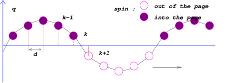
Figure 4: transverse mode.

Let us suppose that plane wave propagation is made of one dimensional wave strings as in fig.(4) (equilibrium distance d, spring constance ${\it K}>0$) with a potential $V(q)=-{1\over 2}{\it K}q^{2}$ for each vacuum electron nearby its stationary position. In the potential $V(q)$, $q$ represents the image on real y axis for the oscillating electron in the internal complex space, and the minus sign is used because vacuum electrons have negative energy and negative mass. Fig.(5) represents the potential $V(q)$ of stationary vacuum electrons for their small oscillations. By the way, minimum action principle in real world need to be modified for those vacuum particle since they have negative energy and mass.

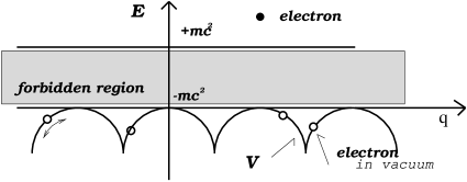
Figure 5: potential energy for small oscillation.

With the lagrangian given as

$$L={1\over 2}\sum_{k=-\infty}^{k=+\infty}[(-m_{e})\dot{q_{k}}^{2}+{\it K}(q_{k-1}-q_{k})^{2}]$$ (7)

and using maximum action principle instead of minimum action principle in real world, the equation of motion is

$$m_{e}\ddot{q}\quad\doteq\quad{\it K}d^{2}\quad{\partial^{2}q\over\partial x^{2}},$$ (8)

where $d\ll 1$. Since tension $S={\it K}d$ and density $\rho={m_{e}\over d}$, it leads to a wave equation as

$${\ddot{q}}\quad=\quad\left({S\over\rho}\right){{\partial^{2}q}\over{\partial x^{2}}},\makebox[28.45274pt]{}$$

where $\sqrt{S/\rho}$ is the propagation speed which is equal to the speed of light in free space.

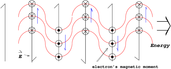
Figure 6: plane wave propagation.

Fig.(6) represents the possible mechanism of light propagation through vacuum in case that one wave length consists of two vacuum electrons. In each energy pulse the electron’s motion let only forward spin flip due to the speed of light.

3.5 Interpretation of photon :  ${E_{\gamma}}=h\nu={p_{\gamma}}c$

In free space let us suppose that the amplitude in each wave train of a plane waves is same for each other and fixed because there is no reason that the amplitudes in plane waves are different. If the energy flux is increased in one wave train, the frequency also increases because the speed of light is constant or the tension $S\propto\rho$. Furthermore, we know that the energy included in one wave length is proportional to the frequency($\nu$)[17] since the electron number in one wave length $n_{e}/\lambda\propto{1\over\nu}$ and the electron’s oscillating velocity $v\propto{\nu}$ in Eqn.(8). What is the proportional constant?

Because we assumed $d\ll 1$ in Eqn.(8), the discrete wave train is presumed as a continuous wave string. For the vibrating string (sinusoidal wave), there is a flow of energy down the string. The power[17] is

$${\it P}=k\omega{\it S}{\it A}^{2}\sin^{2}(kx-\omega t),\makebox[5.69054pt]{}$$

where $A$ is amplitude. Thus, the time average is given as

$$\langle{\it P}\rangle_{av}={1\over 2}k\omega{\it S}{\it A}^{2}.\makebox[56.9055pt]{}$$ (9)

From Eqn.(9), the energy included in one wave length is

$${\it E}_{{}_{\lambda}}=\langle{\it P}\rangle_{av}\makebox[2.84526pt]{}{1\over\nu}=2{\pi}^{2}{\it S}{\it A}^{2}\makebox[2.84526pt]{}{1\over\lambda}.\makebox[5.69054pt]{}$$

On the other hand, ${\it E\/}=pc$ in Special Theory of Relativity. Hence, for one wave length the energy ${\it E\/}_{\lambda}$ is

$$p_{{}_{\lambda}}c=2{\pi}^{2}{\it S}{\it A}^{2}\makebox[2.84526pt]{}{1\over\lambda}.\makebox[56.9055pt]{}$$

The momentum included in one wavelength is

$$p_{{}_{\lambda}}={1\over\lambda}\makebox[5.69054pt]{}\left[2{\pi}^{2}c{\it A}^{2}\left({m_{e}\over d}\right)\right],$$ (10)

in which we used relations, $S=\rho c^{2}$ and $\rho={m_{e}\over d}$. In Section(2), we confirmed : there is a unversal constant for light only if we can assume that the amplitudes of the light wave are same. In other words, if we can assume that there is a basic unit in the amplitude of light, then the constant for one wave length in the wave strings, by which light propagation is made, is minimum and unique. Hence, the universal constant can be expressed as following

$$\makebox[85.35826pt]{}{p_{{}_{\lambda}}}\lambda=2{\pi}^{2}m_{e}c\left({{\it A}^{2}\over d}\right).\makebox[113.81102pt]{}$$ (11)

As we expected, it is a constant indeed as far as the amplitude A is fixed. (Here, $A$ is the amplitude for each wave string.) Considering that the energy included in one wave length can be an energy flux unit in a wave string, it is natural to accept this constant as Planck’s constant($h$). From this calculation we come to know that the amplitude A in each wave string is constant and directly proportional to $\sqrt{d}$. In addition, this relation is independent of the speed of light.

4 physical momentum and wave function in QM.

The inertial mass in Newtonian physics is no more constant in Special Theory of Relativity because energy-momentum-four-vector conservation is assumed in Minkowski space(real world). But the theory says, the mass increase – energy gain – is independent of interactions between two inertial frames or measurements. how is that possible?

If mass $M$ is at the origin of $O^{\prime}$-frame in Fig.(1) and $O^{\prime}$-frame is moving away from $O$-frame with a constant velocity, $v=\beta c$, then the mass in $O$-frame is $M\gamma$ (${\gamma}^{-1}={\sqrt{1-\beta^{2}}}$). Since vacuum particles are interacting with physical object – assumption(6), it is necessary to check out how the distribution of vacuum particles has been changed. However, gravitational interaction between mass $M$ and vacuum particles is repulsive, and thus the potential energy is positive because vacuum particles have negative masses. In the mass rest frame, $O^{\prime}$-frame, the distribution is isotropic in 3-dimensional complex space, but in $O$-frame, it is not isotropic anymore because of the length contraction effect. In $O$-frame, the length contraction effect results in the mass density($\rho$) increase (in absolute value) with the factor of $\gamma$ because total mass of vacuum particles has not been changed, but the volume of space has been changed with the factor of $\gamma^{-1}$.

Firstly, in the rest frame ($O^{\prime}$-frame) ; let us say, the potential energy of the mass $M$ in the interactions with vacuum particles is $|\mit\Phi_{0}|$ – $U(1)$ symmetry. Then, in $O$-frame ; the potential energy $|\mit\Phi|=\gamma\makebox[2.84526pt]{}|{\mit\Phi}_{0}|$ because the mass density in vacuum has been increased with the factor of $\gamma$ – the mass distribution of vacuum particles is assumed as continuous ; the space of vacuum, as infinite. If we compare gravitational potential energies ; in $O^{\prime}$-frame,

$$|{\mit\Phi_{0}}|\makebox[2.84526pt]{}=\makebox[2.84526pt]{}\int_{\mbox{\it vac.\/}}GM\makebox[2.84526pt]{}{\rho(\xi)\over{|\xi|}}\makebox[14.22636pt]{}d{\vec{l}},\makebox[14.22636pt]{}$$

and in $O$-frame,

$$|\mit\Phi| = \int_{\mbox{\it vac.\/}}\gamma\makebox[2.84526pt]{}GM\makebox[2.84526pt]{}{\rho(\xi)\over{|\xi|}}\makebox[14.22636pt]{}d{\vec{l}},$$

$$= \gamma\makebox[2.84526pt]{}|\mit\Phi_{0}|,$$

in which $\xi=r+ir_{i}$, $d{\vec{l}}=dl_{x}dl_{y}dl_{z}$ and $\rho(\xi)$ is the mass density of vacuum particles in absolute value ; then, it is natural to acknowledge the inertial mass increase in the relativistic motion. But, in fact, it is not true because the mass itself is not increasing but has the effect from the vacuum.

In Section(3), vacuum electron-strings vibrations, following imaginary axis, was considered as light wave in real world, and a basic unit in the amplitude was assumed. Then, it came up that the unit of momentum $p$ of light is $\hbar k$ for each $k$. To investigate physical momentum which is possibly related with vacuum particles, let us say, the velocity $v$ is in $x$ direction in Fig.(1) as a simple case. Then, in $O$-frame; the effect of interactions with vacuum particles is moving with the mass $M$ and the interaction is symmetry about $x$ axis. Thus, we can bring (mapping) all interaction effects into the internal complex space. In $O$-frame, the energy formula is

$$E=\sqrt{M^{2}c^{4}+p^{2}c^{2}},\makebox[56.9055pt]{}$$ (12)

$$\makebox[113.81102pt]{}=\makebox[2.84526pt]{}M\gamma c^{2},\makebox[56.9055pt]{}(\gamma={1\over{\sqrt{1-\beta^{2}}}})\makebox[68.28644pt]{}$$

and the momentum, $p=M\gamma\beta c$. In Eqn.(12), the second term in the square root must be come from the interaction between the mass $M$ and vacuum particles. In real world, if the interaction effects with vacuum particles is not considered, only the mass $M$ has all physical quanties, such as energy, momentum, etc. But it needs to be reconsidered in fact that the interaction is included in the system.

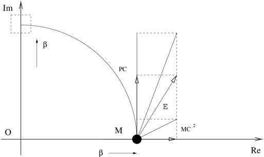
Figure 7: internal complex space with mass $M$ in $O$-frame

Special Relativity says, if the mass $M$ goes to zero, the energy and momentum is also zero. But light still has momentum even though the mass is zero; however, that is a singularity in Eqn.(12) and the equation is not definite when the mass goes to zero with $\beta$ goes to 1. In another words, the momentum is dependent on mass if the mass is not zero, but the momentum is also independent of the mass in light case.

To be consistent in the interpretation of the energy formula in Eqn.(12), the second term, $pc$, should be the energy carried by vacuum particles in a form of bundle of pulse signals following the physical object : Hence, physical momentum in real world is the representation of the interaction with vacuum particles, and in fact vacuum particles carry the momentum on the imaginary axis of the internal complex space. Now there is another question why these two terms are not direct sum in the energy formula. That is because the second term, $pc$, came from the interaction between the mass $M$ and vacuum particles. In Section 3.3, we introduced U(1) symmetry in internal complex space ; that means the phenomenological facts – energy in this case – is invariant under the unitary transformation, U(1), as shown in Fig.(7). The rest mass energy $Mc^{2}$ is not changed in a relativistic motion and thus independent of the second term $pc$, which is on the imaginary axis since the energy comes from the interaction with vacuum particles and the interaction follows the imaginary axis. Meanwhile, there is an interesting point : In magnitude, $pc$ is always greater than the kinetic energy in $O$-frame as far as both are not zero. That is because vacuum particles have negative mass and thus they need some energy when they back to equilibrium states.

If a physical object is in one dimensional motion as above, the effects of the interaction with vacuum particles can be expressed with one dimensional wave function in real world. Let us say, a complex function ${\cal F}(x,t)$ represents the effects, which is following the physical object in a wave form. Hence, the wave function ${\cal F}(x,t)$ represents not a phenomenal wave but the result of summation of infinte number of wave strings in vacuum, and the total energy is $Pc$ which the wave is carrying. The wave function, in general, can be given as

$${\cal F}(x,t)\makebox[5.69054pt]{}=\makebox[5.69054pt]{}{1\over\sqrt{2\pi}}\int_{-\infty}^{\infty}\makebox[5.69054pt]{}{\cal A}(k)\makebox[5.69054pt]{}e^{{i}[kx-\omega(k)t]}\makebox[5.69054pt]{}dk.$$ (13)

Here, ${\cal A}(k)$ is the amplitude of wave string which has wave vector $k$, and $\omega(k)$ is angular velocity. Eqn.(13) is a general expression as long as we can assume superposition principle ; however, there is a condition on $\omega(k)$ because the propagation is in the positive $x$-direction. The condition is

$$\omega(k) \geq \makebox[42.67912pt]{for}k\geq 0,$$

$$\leq \makebox[42.67912pt]{for}k\leq 0,$$

and continuous. Also we can assume $A(0)=0$ and $\omega(0)=0$ without a loss of generality. Since the vacuum is not homogeneous as in plane waves, $\omega(k)\over k$ is not a constant but can be even greater than $c$, speed of light in free space.

Even though the function ${\cal F}(x,t)$ represents the effects from vacuum particles, only real value(ex. energy) has meaning in real world. Now we can find the necessary conditions of ${\cal F}(x,t)$ using a formula, $-{1\over 2}S({{\partial f}\over{\partial x}})({{\partial f}^{*}\over{\partial t}})$ that is average power for a wave, $f(x,t)=Ae^{i(kx-\omega t)}$, where $A$ is amplitude. Let us say, the wave is extended from $x=-L$ to $x=L$(e.g. $L\rightarrow\infty$ later), then the average power of the wave is

$$<Power>\makebox[2.84526pt]{}=\makebox[2.84526pt]{}-{1\over 2}\cdot{S\over 2L}\makebox[2.84526pt]{}\int_{-L}^{L}dx\left({\partial{\cal F}\over{\partial x}}\right)\left({\partial{\cal F}^{*}\over{\partial t}}\right),$$

in which we used the orthogonality of trigonometric functions. Since the average power is the average energy density times group velocity ($v_{g}$), total energy carried by the wave is

$$Pc = M\gamma v_{g}c$$ (14)

$$= {1\over v_{g}}{S\over 2}\int_{-\infty}^{\infty}dk\makebox[2.84526pt]{}|{\cal A}(k)|^{2}k\makebox[2.84526pt]{}\omega(k).$$

In which $P$ is the momentum of the particle, $\delta$-function was used, and $L$ went to infinity. In Eqn.(14) the integration on RHS must be finite as far as the energy on LHS is not infinity. Hence, the integration, $\int_{-\infty}^{\infty}dk|{\cal A}(k)|^{2}$ must be finite because $k\cdot\omega(k)>0$. That is square integrable. Now if we can assume that the function, ${\cal A}(k)$ is continuous in the region( $-\infty<k<\infty$), then we can use Fourier transformation. Hence, the function, ${\cal F}(x)$ is also square integrable because of parseval theorem[18].

In general, Using Fourier transformation, the function ${\cal F}(x,t)$ and the conjugate function ${\cal G}(k,t)$ in $k$-space with $\omega(k)$ are given as

$${\cal G}(k,t)\makebox[5.69054pt]{}=\makebox[5.69054pt]{}{1\over{\sqrt{2\pi}}}\int_{-\infty}^{\infty}\makebox[5.69054pt]{}{\cal F}(x,t)\makebox[5.69054pt]{}e^{-{i}[kx-\omega(k)t]}\makebox[5.69054pt]{}dx,$$

and

$${\cal F}(x,t)\makebox[5.69054pt]{}=\makebox[5.69054pt]{}{1\over{\sqrt{2\pi}}}\int_{-\infty}^{\infty}\makebox[5.69054pt]{}{\cal G}(k)\makebox[5.69054pt]{}e^{{i}[kx-\omega(k)t]}\makebox[5.69054pt]{}dk,\makebox[11.38109pt]{}$$ (15)

where ${\cal G}(k,t)={\cal G}(k)e^{-i\omega(k)t}$. In Eqn.(14), $|{\cal A}(k)|^{2}$ can be interpreted as it is proportional to the energy density in $k$-space in comparison with Eqn.(9), then $|{\cal F}(x)|^{2}$ is also proportional to the energy density because of the symmetry property in Fourier transformation. Therefore, it is natural to interpret that $|{\cal F}(x)|^{2}$ is proportional to probability density in single particle case.

In Eqn.(11) $p\lambda$(Plank’s constant, $h$) is invariant under Lorentz transformation and General Relativity says, we can always construct MCRF(momentary co-moving reference frame), that is, a momentary Lorentz inertial frame. Therefore, we can assume that Plank’s constant($h$) is invariant even under non-uniform space(interaction) because Lorentz transformation is a continuous transformation. With relations for one photon; $p=\hbar k$ and ${\epsilon\/}=\hbar\omega$ (but ${\epsilon\/}\not=pc$.), Eqn.(15) is

$$\psi(x,t)\makebox[5.69054pt]{}=\makebox[5.69054pt]{}{1\over{\sqrt{2\pi\hbar}}}\int_{-\infty}^{\infty}\makebox[5.69054pt]{}\widetilde{\psi}(P)\makebox[5.69054pt]{}e^{{i\over\hbar}[Px-E(P)t]}\makebox[5.69054pt]{}dP.$$ (16)

Here, $P$ and $E(P)$ represent the energy and momentum of the particle, respectively, and a scale transformation was used. In the scale transformation, we used a fact that the system energy is finite. Now, function ${\psi(x,t)}$ is nothing but the wave function in Quantum Mechanics. Furthermore, the uncertainty relations such as $\Delta$$E$ $\Delta$$t\geq$ O and $\Delta$$x$ $\Delta$$p\geq$ O (O$\sim\hbar/2,\hbar,h,\cdots$) can be derived from Eqn.(16) if we know $\psi(x,t)$ or $\widetilde{\psi}(P)$ – as a statistical criterion ; moreover, the relation is consistent to the length contraction effect in Special Relativity – in phenomenological facts.

5 Interpretation and Experiments

5.1 Wave Function Collapse

According to our model interpretation, the wave function in quantum mechanics is not the physical object itself but the representation of the interactions between the physical object and vacuum particles, in which the physical object cannot be isolated without disturbing the wave packet – interaction pattern(symbolic) of the vacuum particles. Therefore, the uncertainty principle is indispensable to describe phenomenological facts. In other words, nature itself – in phenomena – is not apt to the determinism and locality. Thus, we can interpret quantum mechanical formalism as a phenomenological realization of nature in fact that mother nature herself has a statistical property.

Considering that the question of Wave Function Collapse was originated from the view as : the wave function itself is the physical object, and the detection is determined without any time delayed, we don’t need to consider the question because the interacting time($\Delta$$t$) with a detector cannot be zero – wave function never be collapsed – and we are dealing with phenomenological statistics – though it has been the best way up to now.

5.2 One particle double slits experiment

As shown in Fig.(8-2), the slits are at $y=\pm D$ and the screen is at $x=L$. If one particle(ex. neutron) is incident at $y=D$(slit A), the perturbation on stabilized vacuum also affects on slit B simultaneously because of $U(1)$ symmetry and analytic condition as shown in Fig.(8-1). Now, let us say, effects of the perturbation can be given in y-internal complex space as

$$\phi(x,D,\theta,t)\makebox[2.84526pt]{}=\makebox[2.84526pt]{}\int_{-\infty}^{\infty}\left[\sum_{n=-\infty}^{\infty}A_{n}(k,D)e^{in\theta}\right]e^{i(kx-\omega(k)t)}dk,$$ (17)

in which we assume that the slit width is ignorable and the source is far away from the slits. In Eqn.(17) $A_{+n}=A_{-n}$ since results of the interference must be on real y-axis.

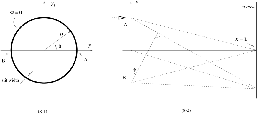
Figure 8: wave function interference

Now, instead of chasing the particle itself we can choose an anternative way – wave function interference – to locate the particle position on the screen ; because the particle cannot be isolated from the wave packet, and the wave function, which is presenting the wave packet, is related to the particle’s position with probability.

If the incident particle is in a relativistic motion($\gamma\gg 1$), then the particle is highly localized with $\Delta$$x\ll$ O but $\Delta$$p\gg$ O. Moreover, duration time of the perturbation on slits is almost instantaneous($\Delta$$t\ll$ O) ; hence, the possible interference pattern can be observed only at around center of the screen($x=L$, $y=0$). To get a simple picture of the interference, let us say, O $\sim\hbar$ and the incident particle is in the relativistic motion($\gamma\gg 1$); thus, the particle is highly localized as $\Delta$$x\ll\hbar$ but $\Delta$$p\gg\hbar$. Then, $\phi_{max}$ in Fig.(8-2) can be estimated using the uncertainty relation($\Delta$$E$ $\Delta$$t\sim\hbar$) : the maximum path difference,

$$\makebox[56.9055pt]{}2Dsin\phi_{max} \doteq v_{g}(\Delta t),$$

$$\sim {v_{g}\hbar\over\Delta E}\makebox[28.45274pt]{}\makebox[85.35826pt]{($\Delta E$ $\Delta t\sim\hbar$)}$$

$$\sim {\hbar c\over\Delta E}\makebox[28.45274pt]{}\makebox[85.35826pt]{($E\sim pc$)}$$

If $\gamma\gg 1$, then $sin\phi\sim\phi$. Thus,

$$\phi_{max}\sim{\hbar c\over 2D(\Delta E)}.$$

Using this fact we can further estimate uncertainty of the particle position on $y$-axis($\Delta$$y$). That is

$$\Delta y\sim\pm{L\hbar c\over 2D(\Delta E)}.$$

Here, $\Delta E$ is the energy uncertainty of the particle, and $\pm$ sign was used because we cannot distinguish which slit the particle has passed through; hence, the position distribution of particles on the screen should be symmetry.

5.3 photoelectric effect

photoelectric effect is called for the interaction between one photon and a bounded electron in a metal. As long as we can assume the interaction is individual – one vacuum-particle-string oscillation and one bounded electron, we can also confirm that the interaction is almost instantaneous ($\Delta$$t\sim\lambda/c$) : According to our intepretation of photon in Eqn.(10)(11), the energy and momentum of one photon is corresponded to the energy and momentum carried by one wave length in vacuum-particle-string oscillation. Therefore, the maximum kinematic energy which the bounded electron can receive is $\sim$ one photon energy, and the interaction time, $\Delta$$t\sim\lambda/c=1/\nu$.

6 Conclusion

The physical entity of wave function in Quantum Mechanics was searched with a model suggested in $\S$(3.1) as following :

Like two sides of a coin - head and tail – we introduced 4-dimensional complex space for physical space and further we defined U(1) symmetry in internal complex space because absolute length is invariant under the rotation in internal complex space. Then, we showed why light speed is constant for all inertial observers and how time dilation effect and length contraction effect in Special Theory of Relativity can be explained; moreover, we interpreted the energy-momentum formula (Eqn.(12)).

When the physical object has kinetic energy, it is wrapped with vacuum particles(vacuum electrons in the model) those of which are interacting with the physical object; the effect of interaction is following the physical object in a wave form, and the velocity($v_{g}$) is the same as that the physical object has. In addition, those vacuum particles, in fact, carry the physical momentum $p$ – momentum of the object conventionally – and kinetic energy $pc$.

In phenomena, we cannot single out the physical object without disturbing vacuum particles, those of which are wrapping the physical object. Therefore, it is indispensable to accept uncertainty principle and de Broglie matter wave in Quantum Mechanical formalism to describe phenomena. In other words, nature itself has a statistical property intrinsically, which means indeterminism and non-locality in phenomena. Thus, the wave function in Quantum Mechanics is not the physical object itself but an alternative descritpion – especially in microphysics – for vacuum particles interacting with the physical object.

In $\S$(5), fundamental questions – Wave Function Collapse, one-particle-double-slits experiment – mentioned in the introduction, and photoelectric effect were reviewed. Especially, one-particle-double-slits experiment was explained, and a possible interference pattern was also estimated.

Figure Caption

• lorentz transformation with arbitrary $\vec{\beta}$.

• 3-dimensional complex space($\beta=v/c$).

• internal and coupled complex space.

• light propagation(transverse mode).

• potential energy of vacuum electrons for small oscillation.

• plane wave propagation.

• internal complex space with mass $M$ in $O-$frame.

• wave function interference.

References

- [1] Thomas Brody, The Philosophy Behind Physics, (Springer-Verlag Berin Heidelberg, 1993), pp. 159-184.
- [2] J.S. Bell, Speakable and unspeakable in quantum mechanics, (Cambridge University Press 1987), pp. 169-172.
-
[3]
Paul Marmet, Absurdities in Modern Physics :
A Solution,
(ISBN 0-921272-15-4,
Les Éditions du Nordir, c/o R. Yergeau, 165 Waller, Ottawa, Ontario K1N 6N5, 1993),
pp. 13-31. - [4] David Bohm, Physical Review, vol. 85, (1592) 166
- [5] Bryce S. DeWitt, Physics Today, September, (1970) 30
- [6] Plato, The Republic : Book VII
- [7] Plato, The Republic(translated and edited by Raymond Larson), (AHM Publishing Co. 1979), pp. vi, pp. 174-201.
-
[8]
Paul Marmet, Absurdities in Modern Physics :
A Solution,
(ISBN 0-921272-15-4,
Les Éditions du Nordir, c/o R. Yergeau, 165 Waller, Ottawa, Ontario K1N 6N5, 1993),
pp. 134-138. - [9] P.A.M Dirac, Proc. Roy. Soc. (London), A 126, (1930) 360.
- [10] James D. Bjorken and Sidney D. Drell, Relativistic Quantum Mechanics, (McGraw-Hill), pp. 64-75.
- [11] James D. Bjorken and Sidney D. Drell, Relativistic Quantum Mechanics, (McGraw-Hill), pp. 70-71.
- [12] J. D. Jackson, Classical Electrodynamics, (John Wiley & Sons, Inc. 1975) pp. 42.
- [13] Philippe Dennery and André Krzywicki, Mathematics for Physicists, (Harper & Row publishers, 1967), pp.14-18.
- [14] Ruel V. Churchill, James W. Brown, Roger F. Verhey, Complex Variables and Applications, (McGraw-Hill, Inc., 1974) pp. 39-49.
- [15] Ruel V. Churchill, James W. Brown, Roger F. Verhey, Complex Variables and Applications, (McGraw-Hill, Inc., 1974) pp. 283-290. ; Philippe Dennery and André Krzywicki, Mathematics for Physicists, (Harper & Row publishers, 1967), pp. 76-82.
- [16] Philippe Dennery and André Krzywicki, Mathematics for Physicists, (Harper & Row publishers, 1967), pp. 30-31.
- [17] Keith R. Symon, Mechanics (Third Edition), (Addison-Wesley publishing Co.,1980), pp. 295-304.
- [18] Philip M. Morse, Herman Feshbach, Methods of Theoretical Physics, (McGraw-Hill Book Co., Inc. 1953), pp. 455-459.