Effects of noise on quantum error correction algorithms

Abstract

It has recently been shown that there are efficient algorithms for quantum computers to solve certain problems, such as prime factorization, which are intractable to date on classical computers. The chances for practical implementation, however, are limited by decoherence, in which the effect of an external environment causes random errors in the quantum calculation. To combat this problem, quantum error correction schemes have been proposed, in which a single quantum bit (qubit) is “encoded” as a state of some larger number of qubits, chosen to resist particular types of errors. Most such schemes are vulnerable, however, to errors in the encoding and decoding itself. We examine two such schemes, in which a single qubit is encoded in a state of $n$ qubits while subject to dephasing or to arbitrary isotropic noise. Using both analytical and numerical calculations, we argue that error correction remains beneficial in the presence of weak noise, and that there is an optimal time between error correction steps, determined by the strength of the interaction with the environment and the parameters set by the encoding.

1 Introduction

Soon after the discovery of fast quantum algorithms for factorization [1], it was realized that the efficiency of quantum computers depends crucially on the control of errors during a computation. This is not surprising in itself, since classical computers also require an active monitoring of errors to operate properly. However, the dissipative techniques used in classical error correction destroy the superpositions necessary for quantum computation. This problem stimulated an important effort in the direction of quantum error correction. In the last year or so, after the initial discovery of quantum error correction codes by Shor [2] and Steane [3, 4], significant progress has been made in the development and understanding of these codes. Much attention has been devoted to the construction of codes using a variety of different techniques to convert classical codes into quantum codes [5, 6] and providing a mathematical description of large families of these codes [7, 8]. Minimal codes, that correct only one or a few errors, were also derived [9, 10]. Most of this work addresses the issue of how most efficiently to preserve a quantum state in a noisy environment given that encoding and decoding can be done in an error-free way. Only a few recent papers have addressed the possibility of encoding and decoding in the presence of noise [11, 12]; these fault-tolerant schemes are relatively complicated and involve many more qubits than the earlier simple codes. It is therefore unlikely that we will see an experimental implementation of these more elaborate proposals in the near term. On the other hand, the issue of errors arising during encoding and decoding has only been partially investigated in the simplest error correcting codes proposed so far [13]. These are the codes that could be implemented in a near-future quantum computer. The aim of this work is to bridge this gap, and provide numerical as well as algebraic evidence that for certain regimes of noise, error correction is worthwhile even when noise is present during the encoding and decoding steps, as will be the case in any real experiment.

This paper is organized as follows. Section 2 reviews the effect of unwanted environmental coupling on a quantum computer, its description in terms of master equations, and the fundamental operation of error correcting codes. Section 3 presents an analytical discussion of the effect of errors on an evolution consisting of encoding, free evolution of an encoded qubit, and decoding, with noise present at all stages. The concept of a quantum trajectory is described in section 4, where numerical simulation algorithms are presented using two unravelings of the master equation (quantum jumps and quantum state diffusion) as well as direct numerical solution of the master equation. The numerical methods are found to be in reasonable agreement with the analytical model.

2 Noise and error correction

2.1 Decoherence

A quantum system in complete isolation evolves according to the Schrödinger equation

$${{d{|\psi\rangle}}\over{dt}}=-{i\over\hbar}{\hat{H}}{|\psi\rangle},$$ (1)

where ${|\psi\rangle}$ is the state of the system (in this case a quantum computer) and ${\hat{H}}$ is the Hamiltonian (in this case representing the action of the quantum “gates;” in general, ${\hat{H}}$ will be time-dependent). This evolution is unitary.

Unfortunately, the approximation of a system being isolated is only good for microscopic noninteracting systems. As a system becomes larger and more complicated, the effects of the environment become more important.

Consider the example of a single qubit interacting with an external environment. The state of the qubit is described by a vector in a two-dimensional Hilbert space. A convenient basis is the canonical basis ${\cal B}=\{{|0\rangle},{|1\rangle}\}$. Suppose that the qubit is initially in a superposition state $\alpha{|0\rangle}+\beta{|1\rangle}$ and the environment in some unknown state ${|A\rangle}$. As the system and environment interact, the initial product state $(\alpha{|0\rangle}+\beta{|1\rangle})\otimes{|A\rangle}$ can evolve into an entangled state $\alpha{|0\rangle}\otimes{|B_{0}\rangle}+\beta{|1\rangle}\otimes{|B_{1}\rangle}$, where the environment has become correlated with the state of the system (more realistic models of coupling with the environment can be found in Ref [14]). The system can no longer be described by a state on its own. Normally, an environment is very complicated, containing many degrees of freedom, so it is likely that ${|B_{0}\rangle}$ and ${|B_{1}\rangle}$ will be orthogonal (or very nearly so). Thus, if we trace out the environment degrees of freedom, an ensemble of our systems of interest is left in a mixture, described by a reduced density matrix

$${\hat{\rho}}=|\alpha|^{2}{|0\rangle}{\langle 0|}+|\beta|^{2}{|1\rangle}{\langle 1|}.$$ (2)

In effect, the environment has measured the value of the qubit, and the superposition has been destroyed. In this case, the evolution of the reduced system is no longer unitary; and algorithms which depend on the unitarity of the evolution, such as the Shor algorithm, will no longer function.

The general effects of the environment on a quantum system can be very complicated and difficult to describe. However, a useful approximation is to assume that the effects of the environment are Markovian, or local in time. In this case, it is possible to describe the evolution of the reduced density matrix by a master equation of Lindblad form [15]

$${d\over{dt}}\,\hat{\rho}=-{i\over\hbar}[\hat{H},\hat{\rho}]+\sum_{j}\left(\hat{L}_{j}\hat{\rho}\hat{L}_{j}^{\dagger}-{1\over 2}\hat{L}_{j}^{\dagger}\hat{L}_{j}\hat{\rho}-{1\over 2}\hat{\rho}\hat{L}_{j}^{\dagger}\hat{L}_{j}\right)\;,$$ (3)

where $\hat{H}$ is the system Hamiltonian and the $\hat{L}_{j}$ are the Lindblad operators representing the interaction with the environment. This Markovian approximation is generally very good when the environment is large compared with the system and the interaction between them is fairly weak. It might fail, however, for some realizations of quantum computers.

What kinds of Lindblad operators typically occur in (3)? This depends on the physics of the system, but certain operators are common in quantum optical and atomic physics models. One normal effect of environmental interaction is dissipation, as in spontaneous emission. If the qubit state ${|1\rangle}$ represents an excited state, there will be a Lindblad operator proportional to the lowering operator, of the form ${\hat{L}}=\sqrt{\kappa}{\hat{\sigma}}_{-}$, (${\hat{\sigma}}_{-}{|1\rangle}={|0\rangle}$ and ${\hat{\sigma}}_{-}{|0\rangle}=0$). The qubit will tend to the ground state in the long term, regardless of its initial state. If the environment has a non-zero temperature, there is the possibility of thermal excitations as well, represented by another Lindblad operator proportional to the raising operator ${\hat{\sigma}}_{+}={\hat{\sigma}}_{-}^{\dagger}$ .

Even if the rate of dissipation is small enough to be negligible, the environment can still act to destroy superpositions. As we saw in (2), correlations which develop with the environment can randomly dephase the basis states ${|0\rangle}$ and ${|1\rangle}$. This process is represented by a Lindblad operator proportional to the $z$ Pauli matrix, ${\hat{L}}=\sqrt{\kappa}{\hat{\sigma}}_{z}$, (${\hat{\sigma}}_{z}{|0\rangle}=-{|0\rangle}$ and ${\hat{\sigma}}_{z}{|1\rangle}={|1\rangle}$).

The most general interaction will reduce the qubit ensemble density operator to the one at the center of the Bloch sphere. The individual (pure) states of the members of the ensemble can be viewed as moving randomly on the surface of the sphere. This effect is represented by isotropic noise, with three Lindblad operators proportional to ${\hat{\sigma}}_{x},{\hat{\sigma}}_{y}$ and ${\hat{\sigma}}_{z}$, used in studying the depolarizing channel [7, 10]. The exact choice of model is determined by the physics of the quantum computer and its environmental interactions.

2.2 Error correcting codes

For a qubit ${|\psi\rangle}$, the most general form of single-qubit error induced by the environment can be written as

$${|\psi\rangle}\rightarrow{\hat{E}}{|\psi\rangle},$$ (4)

where ${\hat{E}}$ is an arbitrary operator which can be decomposed as

$${\hat{E}}=e_{1}\leavevmode\hbox{\normalsize 1\kern-4.6pt\large 1}+e_{x}{\hat{\sigma}}_{x}+e_{y}{\hat{\sigma}}_{y}+e_{z}{\hat{\sigma}}_{z},$$ (5)

where 11 is the identity and the ${\hat{\sigma}}_{i}$ are the Pauli matrices. In the simplest case (when one wants to protect a single qubit), error correcting codes consist in encoding the basis states ${|0\rangle}$ and ${|1\rangle}$ of a qubit in well chosen states of several qubits:

$$\begin{array}[]{l}{|0\rangle}\rightarrow{|C_{0}\rangle}\\ {|1\rangle}\rightarrow{|C_{1}\rangle},\end{array}$$ (6)

where ${|C_{0}\rangle}$ and ${|C_{1}\rangle}$ belong to the extended Hilbert space of several qubits. Numerous techniques for constructing these codes have appeared in the recent literature [16]. These error correcting techniques commonly assume that the encoding step (i.e. the operation by which a single qubit in state $\alpha{|0\rangle}+\beta{|1\rangle}$ is entangled with additional qubits to form the state $\alpha{|C_{0}\rangle}+\beta{|C_{1}\rangle}$) as well as the decoding and correcting steps are done in a noiseless environment. The issue of noisy encoding and decoding has been addressed little outside the context of fault-tolerant techniques, which require many more qubits [11, 12]. In this work, we will focus on earlier and more compact codes, and analyze the issue of noisy encoding and decoding. In the next two sections we review the two codes that we have analyzed.

2.3 Dephasing noise

If one seeks to protect a qubit against a dephasing noise (in Eq. 5 this is equivalent to setting $e_{y}=e_{z}=0$), it can be shown that the smallest possible code requires three qubits to encode the states ${|0\rangle}$ and ${|1\rangle}$ of the initial qubit. This carefully chosen superposition was first proposed by Shor [2]. We use here an equivalent version found in Ref. [5, 17], in which

$$\begin{array}[]{l}{|0\rangle}\rightarrow{|C_{0}\rangle}={|000\rangle}+{|001\rangle}+{|010\rangle}+{|011\rangle}+{|100\rangle}+{|101\rangle}+{|110\rangle}+{|111\rangle}\\ {|1\rangle}\rightarrow{|C_{1}\rangle}={|000\rangle}-{|001\rangle}-{|010\rangle}+{|011\rangle}-{|100\rangle}+{|101\rangle}+{|110\rangle}-{|111\rangle}\end{array}$$ (7)

(normalization factors have been omitted). We use the networks for encoding and for decoding/correcting shown in Fig. 1. Initially, the first qubit is in the state $\alpha{|0\rangle}+\beta{|1\rangle}$. This is the state we wish to protect. The second and third qubits are in the state ${|0\rangle}$. The result of the encoding network is the three-qubit state $\alpha{|C_{0}\rangle}+\beta{|C_{1}\rangle}$.

In these figures we choose the various quantum gates in such way that they can be described by simple Hamiltonians. The gates $A$ correspond to the unitary operation

$$U_{A}=\frac{1}{\sqrt{2}}\left(\begin{array}[]{cc}1&1\\ 1&-1\end{array}\right)$$ (8)

effected by the Hamiltonian $H_{A}=\frac{\pi}{2}(\frac{1}{\sqrt{2}}({\hat{\sigma}}_{x}-{\hat{\sigma}}_{z})+\leavevmode\hbox{\normalsize 1\kern-4.6pt\large 1})$ acting for one unit of time. Similarly the gate $U_{y}$ corresponds to the unitary operation

$$U_{y}=\frac{1}{\sqrt{2}}\left(\begin{array}[]{cc}1&1\\ -1&1\end{array}\right),$$ (9)

generated by the Hamiltonian $H_{y}=-\frac{\pi}{4}{\hat{\sigma}}_{y}$ acting for one unit of time.

Please note that these matrices are represented in the basis $\{{|0\rangle},{|1\rangle}\}$, as is the convention in the quantum computation literature. Unfortunately, this is precisely the opposite of the usual convention for the Pauli matrices. For this paper we have retained the quantum computation basis, as we do not present the Pauli matrices explicitly, but this notational conflict should be resolved.

The two-bit gates of the network correspond to controlled phase shifts. These are represented in the canonical basis ${\cal B}=\{{|00\rangle},{|01\rangle},{|10\rangle},{|11\rangle}\}$ by the unitary operator

$$U=\left(\begin{array}[]{cccc}1&0&0&0\\ 0&1&0&0\\ 0&0&1&0\\ 0&0&0&-1\\ \end{array}\right),$$ (10)

generated by the Hamiltonian $H=\pi P_{{|1\rangle},i}\otimes P_{{|1\rangle},j}$, where $i$ and $j$ designate the two qubits on which the gate acts and $P_{{|1\rangle}}=\frac{1}{2}(\leavevmode\hbox{\normalsize 1\kern-4.6pt\large 1}+{\hat{\sigma}}_{z})$ is the projector on state ${|1\rangle}$. In this case a state ${|i,j\rangle}$ picks up a phase $\pi$ iff both qubits are in state ${|1\rangle}$. Variants on this gate can be obtained by replacing either or both of the projection operators with $P_{{|0\rangle}}$ in the definition of the Hamiltonian.

The decoding network is just the reverse of the encoding network. After completing the sequence of gates, qubits 2 and 3 can be measured to identify the error, which is followed by an adequate correction of the first qubit [5, 17].

Figure 1: Encoding and decoding networks from [17]. The graphical conventions are similar to those in Ref. [18]. The gate $U_{A}$ represents the operation ${|0\rangle}\rightarrow{|0\rangle}+{|1\rangle}$ and ${|1\rangle}\rightarrow{|0\rangle}-{|1\rangle}$ (cf. Eq. 8 in the text). The gate $U_{y}$ is a $\pi$ rotation of the qubit along the $y$ axis (Eq. 9). The two-bit gates denoted by a line and two black dots are “control-phase” gates. They change by $\pi$ the phase of a quantum state only when both qubits are in state ${|1\rangle}$ (cf. Eq. 10).

2.4 Arbitrary noise

In the previous section we have shown how to protect a single qubit against dephasing noise (i.e., noise generated by a single Lindblad operator proportional to ${\hat{\sigma}}_{z}$). If one seeks to protect a single qubit against an arbitrary error of the form (5), such as isotropic noise, then five qubits are necessary to encode a state. Different versions of these codes (all equivalent) have been proposed [9, 10]. We choose to implement an equivalent version of the code given by [9]:

$$\begin{array}[]{ll}{|C_{0}\rangle}=&|b_{1}\rangle|00\rangle-|b_{3}\rangle|11\rangle+|b_{5}\rangle|01\rangle+|b_{7}\rangle|10\rangle\\ {|C_{1}\rangle}=-&|b_{2}\rangle|11\rangle-|b_{4}\rangle|00\rangle-|b_{6}\rangle|10\rangle+|b_{8}\rangle|01\rangle,\end{array}$$ (11)

where $|b_{1\atop 2}\rangle=(|000\rangle\pm|111\rangle)$, $|b_{3\atop 4}\rangle=(|010\rangle\pm|101\rangle)$, $|b_{5\atop 6}\rangle=(|001\rangle\pm|110\rangle)$, $|b_{7\atop 8}\rangle=(|011\rangle\pm|100\rangle)$. The implementation of this code is done in a way similar to the three bit case. In the first stage, a qubit in state ${|\psi_{in}\rangle}=\alpha{|0\rangle}+\beta{|1\rangle}$ is entangled with four additional qubits (initially in state ${|0\rangle}$) to produce the state $\alpha{|C_{0}\rangle}+\beta{|C_{1}\rangle}$. This is done through the network of Fig. 2. Similar gates as in the previous section are used. Note that some of the control-phase gates change the phase when a qubit is in state ${|0\rangle}$ rather than in state ${|1\rangle}$, unlike the three qubit code.

The decoding network is also given by Fig. 2 with the gate operations performed in the reverse order (this is possible because each gate appearing in the network is self-adjoint). After decoding, qubits 2 to 5 are measured and, depending on the outcome, an appropriate correction is applied to return the first qubit to the correct state. (For a complete description of this code, see Ref. [9].)

Figure 2: Encoding network for the five bit error correcting code from Ref. [9]. The network has been adapted in order to provide a more natural implementation of the gates in term of Hamiltonians. The decoding network is identical to the encoding one read backwards. Dashed line indicate units of time, i.e., all the gates between two dashed line can be effected in one unit of time. The total encoding (or decoding) time is therefore 10 units. The gate that appear at time 2 is a generalization of the control-phase gate; it imparts a phase factor of $\pi$ to the quantum state only if all qubits denoted by a black dot are in state ${|1\rangle}$. It will effect the operation ${|1,i_{2},1,1,i_{5}\rangle}\rightarrow-{|1,i_{2},1,1,i_{5}\rangle}$ and leave all others states untouched. The gate at time 3 is a variation: the qubits indicated by a white dot act as controls when they are in state ${|0\rangle}$ rather than ${|1\rangle}$.

3 Analytic considerations

Given that error correction can be implemented through encoding a one-qubit state into an $n$-qubit state, it is instructive to consider some simple analytic conditions for the case of imperfect encoding, decoding and correction. These conditions will complement our numerical results and indicate the parameter ranges for which correction is potentially useful.

Subsections 3.1-3.3 discuss a simple approach. To model the imperfect operation of the code, we assume that the decoherence which acts during the encoding and decoding does not get corrected at all. Subsection 3.4 examines the validity of modeling the influence of the environment as instantaneous errors of the type (4), and demonstrates that this type of treatment can be made consistent with the master equation (3) to low order.

3.1 Perfect single error correction

First we need a benchmark. For simple decoherence, the probability that a single qubit remains error free for a time $T$ is defined to be

$$p_{snc}={\rm e}^{-\kappa_{n}T}\;.$$ (12)

The “$s$” stands for success—it could be that the aim is to successfully store the qubit for time $T$, or to transmit it down a channel where the time taken for this is $T$—and “$nc$” indicates that no correction procedure is applied to the qubit. If $\xi$ is the probability of an error and $\xi\ll 1$, then $\xi=1-p_{snc}\approx\kappa_{n}T$.

The subscript $n$ on the decoherence rate $\kappa_{n}$ denotes the fact that the number of qubits needed for encoding is determined by the type of noise. The relevant examples presented in the previous section are $n=3$ for phase noise (modeled by $\hat{L}_{1}=\sqrt{\kappa}{\hat{\sigma}}_{z}$) and $n=5$ for isotropic noise (modeled by $\hat{L}_{1}=\sqrt{\kappa}{\hat{\sigma}}_{x}$ , $\hat{L}_{2}=\sqrt{\kappa}{\hat{\sigma}}_{y}$ and $\hat{L}_{3}=\sqrt{\kappa}{\hat{\sigma}}_{z}$). We define the mismatch between the ensemble at time $T$ and that $T=0$ to be

$$m_{nec}(T)\equiv 1-{\langle\psi_{ini}|}\rho{|\psi_{ini}\rangle},$$ (13)

where ${|\psi_{ini}\rangle}$ is the initial pure state at time $T=0$. In the phase noise example, an ensemble of single qubits given by ${|\psi_{ini}\rangle}=2^{-1/2}({|0\rangle}+{|1\rangle})$ decoheres so that the mismatch $m_{nec}$ is easily shown to be

$$m_{nec}(T)=\frac{1}{2}\left(1-{\rm e}^{-2\kappa T}\right)\;.$$ (14)

We therefore obtain $\kappa_{3}=2\kappa$, since the exponentially decaying term in the mismatch can be identified with the probability that the system remains error free. In the isotropic noise case, the same initial ensemble decoheres and exhibits a mismatch of

$$m_{nec}(T)=\frac{1}{2}\left(1-{\rm e}^{-4\kappa T}\right)$$ (15)

and so we identify $\kappa_{5}=4\kappa$. The particular choice of initial state is made so that it exhibits sensitivity to phase or to isotropic noise. It is also used in the numerical simulations, so we compare like with like.

Consider now the $n$-qubit encoding and decoding procedure which is able to correct perfectly for a single error in one of the $n$ qubits, but fails if there are two or more errors. Using this procedure, the probability of the successful survival of a single encoded qubit state for time $T$ is the sum of the zero error and one error probabilities;

$$p_{sc}(n)={\rm e}^{-n\kappa_{n}T}\;+\;n{\rm e}^{-(n-1)\kappa_{n}T}\left(1-{\rm e}^{-\kappa_{n}T}\right)\;.$$ (16)

(Each qubit is assumed to suffer the same decoherence rate $\kappa_{n}$.) Clearly, if $\kappa_{n}T\ll 1$, perfect error correction is worthwhile because $p_{sc}(n)$ is closer to unity than is $p_{snc}$. ($p_{snc}\approx 1-\kappa_{n}T$, whereas $p_{sc}\approx 1-\frac{n(n-1)}{2}\kappa_{n}^{2}T^{2}$ .) For the case $n=3$ the crossover point arises when $p_{snc}=p_{sc}(3)$, which yields $\kappa_{3}T=\ln 2$. For the case $n=5$, $p_{snc}=p_{sc}(5)$ gives $\kappa_{5}T=0.14$. Any realistic systems are likely to be well down in $\kappa_{n}T$ from these values and so would certainly benefit from perfect error correction.

3.2 Imperfect error correction

Consider now the case where the encoding (E) and decoding (D) for the error correction procedure take a finite amount of time. Let this be $T\delta$, so $\delta$ is the dimensionless fraction of time taken by one full E+D stage. D may be essentially the inverse of E and so each may take $\delta/2$, but this is not crucial. The decoherence rate could well differ during E and D; we denote it by $\kappa_{n}^{\prime}$. The environment seen by the qubits may be different when the encoding and decoding interactions are occurring. The point to note is that errors which occur during the E+D stage are unwelcome. We assume that they don’t get corrected and so contribute directly to the error rate for qubit system.

If the problem at hand is the storage of a given qubit state for time $T$, it seems reasonable to allow E+D to be part of $T$, so the encoded $n$-qubit state is then kept for $(1-\delta)T$. Alternatively, if the goal is to propagate a qubit state down a channel where the time for transmission is $T$, it would seem to be more realistic to add on $T\delta$, so the whole process takes $(1+\delta)T$. This distinction does not appear to be crucial, but we examine both cases.

3.2.1 Storage with imperfect correction

The probability $s$ that there is no error in this system is the product of the probability of all $n$ qubits surviving $T\delta$ at a decoherence rate of $\kappa_{n}^{\prime}$ with the probability of zero or one error (which can be corrected) during the time $(1-\delta)T$ at a rate $\kappa_{n}$. Using (16), this gives

$$s_{sc}(n)={\rm e}^{-n\kappa_{n}^{\prime}T\delta}\left(n{\rm e}^{-(n-1)\kappa_{n}(1-\delta)T}\;-\;(n-1){\rm e}^{-n\kappa_{n}(1-\delta)T}\right)\;.$$ (17)

This reduces to $p_{sc}(n)$ given in (16) as $\delta\rightarrow 0$.

To make a simple comparison, let $\kappa_{n}^{\prime}=\kappa_{n}$. Equating $s_{sc}(n)$ to $p_{snc}(n)$, the aim is to find the crossover value for $\delta$. Clearly $\delta$ is about $1/n$ ; the next order correction in $\kappa_{n}T$ gives

$$\delta=\frac{1}{n}\;-\;\frac{(n-1)^{3}}{2n^{2}}\kappa_{n}T\;+\;...$$ (18)

Provided that $\delta$ stays below this value, there should be benefit from error correction even though errors may occur during E+D. However, if $\delta$ exceeds this value, the performance of the procedure is actually worse than doing no correction to a single qubit. For the cases $n=3$ and $n=5$ and provided that $\kappa_{n}T\ll 1$, the bounds on $\delta$ are not very constraining. Practical systems would probably have $\delta\ll 1$ and so would operate in the regime where imperfect correction is beneficial.

3.2.2 Transmission with imperfect correction

The probability $t$ that there is no error in this system is the product of the probability of all $n$ qubits surviving $T\delta$ at a decoherence rate of $\kappa_{n}^{\prime}$ with the probability of zero or one error (which can be corrected) during the transmission time $T$ at a rate $\kappa_{n}$. Using (16), this gives

$$t_{sc}(n)={\rm e}^{-n\kappa_{n}^{\prime}T\delta}\left(n{\rm e}^{-(n-1)\kappa_{n}T}\;-\;(n-1){\rm e}^{-n\kappa_{n}T}\right)\;.$$ (19)

This also reduces to $p_{sc}(n)$ given in (16) as $\delta\rightarrow 0$.

To again make a simple comparison, let $\kappa_{n}^{\prime}=\kappa_{n}$. Equating $t_{sc}(n)$ to $p_{snc}(n)$, the aim is to find the crossover value for $\delta$. Once again $\delta$ is about $1/n$ ; the next order correction in $\kappa_{n}T$ gives

$$\delta=\frac{1}{n}\;-\;\frac{(n-1)}{2}\kappa_{n}T\;+\;...$$ (20)

The conclusion for transmission is the same as that for storage. Practical systems with $\kappa_{n}T\ll 1$ and $\delta\ll 1$ will be in the regime where correction is beneficial.

3.2.3 Single correction optimization

In the numerical simulations presented in Sect. 4, the encoding and decoding take a set amount of time, rather than a set fraction of $T$. We therefore define an alternative parameterization of the time taken for E+D, setting $T\delta=\Delta$. Our analytic expressions can be viewed either in terms of $\delta$ or of $\Delta$, whichever is most appropriate.

Here we just give a simple analytic result, optimizing the time $T$ to achieve the most benefit from correction. Assuming that the time taken for E+D is fixed at $\Delta$, what is the optimum $T$? We find this by maximizing the ratio $R$ of the mismatch without correction to the mismatch with correction

$$R\equiv\frac{1-p_{snc}(n)}{1-s_{sc}(n)},$$ (21)

and similarly for the transmission case. The maximum of $R$ is an indicator of where (imperfect) error correction is giving the maximum benefit in comparison to performing no correction at all; it is one of the measures we use in our numerical work. To the lowest approximation (assuming that $\kappa_{n}T\ll 1$ always), the optimum $T$ is the same for both storage and transmission, and is given by

$$T_{opt}\approx\left(\frac{2\Delta}{(n-1)\kappa_{n}}\right)^{1/2}\;.$$ (22)

Obviously, if the error correction is perfect (effectively taking zero time), we arrive at the conclusion that it should be performed as often as possible; $T_{opt}=0$. However, for cases of practical interest (finite $\Delta$) this is not so as $T_{opt}$ is then finite. The dependence of $T_{opt}$ on $\kappa$ will be compared to our numerical simulations in Fig. 6.

3.3 $N$-correction procedure

The basic aim of error correction (within the context of this paper) is to maximize the probability of success, storing or transmitting the state as well as possible. The parameters $T$, $\kappa$, $\kappa^{\prime}$, $n$ and $\delta$ are therefore set by the problem at hand. $T$ is set by the total length of the transmission channel or the total required storage time. (The latter might be the time for which the state “idles” between interactions in a larger quantum computation; for such a case the simple error correction procedures discussed in this paper would be sufficient to keep it coherent while it idles.) The decoherence is set by the environment. $n$ and $\delta$ will be set by the chosen correction scheme and its physical realization. However, there is still some freedom. Given all the parameters above, the number of correction procedures applied during $T$ can be varied.

3.3.1 Perfect error correction

Consider then the problem of optimizing error correction to achieve the greatest probability of successful storage or transmission of a qubit state, given the freedom to apply an arbitrary number $N$ of E+D procedures during the time $T$. Assume that these are spaced out equally. For the case of perfect error correction, where $\delta=0$ so there is no possibility of an error occurring during E+D, it is obviously beneficial to apply as many corrections as possible. The probability of success for $N$ applications is

$$p_{Nsc}(n)=\left(n{\rm e}^{-(n-1)\kappa_{n}T/N}\;-\;(n-1){\rm e}^{-n\kappa_{n}T/N}\right)^{N}\;.$$ (23)

This maximizes for $N\rightarrow\infty$, tending to unity independent of the value of $n$, and is consistent with our observation that $T_{opt}=0$ when $\Delta=0$. Such behavior is like the “Zeno” or “watchdog” effect; there is no change at all from the initial state as $N\rightarrow\infty$.

3.3.2 Storage with imperfect correction

In any realistic situation we will have $\delta>0$. For any finite value of $\delta$, there is a non-vanishing probability of introducing a non-correctable error for each application of E+D, so it seems intuitively reasonable that there should be an optimum value of $N$. Also, for the case of storage, it makes sense to impose $N\delta<1$, or else the time taken for $N$ applications of E+D will exceed the time for which the qubit is stored. Practically, it is likely that $N\delta\ll 1$ would hold.

The generalization of (17) to $N$ equally spaced corrections is

$$s_{Nsc}(n)={\rm e}^{-nN\kappa_{n}^{\prime}T\delta}\left(n{\rm e}^{-(n-1)\kappa_{n}((1/N)-\delta)T}\;-\;(n-1){\rm e}^{-n\kappa_{n}((1/N)-\delta)T}\right)^{N}\;.$$ (24)

For the simplest case of a decoherence rate always equal to $\kappa_{n}$, equating the derivative (with respect to $N$) to zero, keeping only the leading terms and rearranging to give the optimum $N$ yields

$$N\approx\left(\frac{(n-1)\kappa_{n}T}{2\delta}\right)^{1/2}=\left(\frac{(n-1)\kappa_{n}}{2\Delta}\right)^{1/2}T\;.$$ (25)

Note that this is consistent with our result (22), if we identify $T_{opt}$ with $T/N$.

3.3.3 Transmission with imperfect correction

Since the time for $N$ applications of E+D does not eat into $T$, but adds to it for transmission, there is not the absolute requirement that $\delta<(1/N)$. However, for practical cases it is likely that $N\delta\ll 1$, the same as for storage. The generalization of (19) to $N$ equally spaced corrections is

$$t_{Nsc}(n)={\rm e}^{-nN\kappa_{n}^{\prime}T\delta}\left(n{\rm e}^{-(n-1)\kappa_{n}T/N}\;-\;(n-1){\rm e}^{-n\kappa_{n}T/N}\right)^{N}\;.$$ (26)

The optimum $N$ is again given by (25), although there are differences at the next order.

3.3.4 $N$-step optimization

As expected, there is an optimum number $N$ of corrections to apply when these procedures themselves are imperfect. When $N\delta\ll 1$, the optimum is the same for the storage and the transmission scenarios.

It is interesting to substitute back the optimum $N$ of (25), to obtain the maximum achievable transmission and storage success probabilities. At the first order of approximation they are equal and given by

$$\max_{N}(s_{Nsc}(n))\approx\max_{N}(t_{Nsc}(n))\approx\exp\left[-n\kappa_{n}T\left(2(n-1)\delta\kappa_{n}T\right)^{1/2}\right]$$

$$\approx 1-n\kappa_{n}T\left(2(n-1)\delta\kappa_{n}T\right)^{1/2}\;.$$ (27)

Thus, within the simple framework used here, the minimum probability for a qubit state to incur an error in a total (storage or transmission) time $T$ is approximately $n\kappa_{n}T\left(2\delta(n-1)\kappa_{n}T\right)^{1/2}$. For cases of practical interest, where this probability is small (and so the success probabilities are close to unity), this is a good approximation.

It is worth noting that, because of the square root in (25), the optimum $N$ does not grow too quickly. For example, with phase noise at $\kappa=10^{-5}$ (i.e. $n=3$ and $\kappa_{3}=2\kappa$), and with $\Delta=10$ and a total time of $T=10^{4}$, the minimum qubit error probability (calculated using (27)) of 0.017 arises from applying $N\sim 14$ corrections. With isotropic noise at the same $\kappa$ (i.e. $n=5$ and $\kappa_{5}=4\kappa$), and with $\Delta=20$ and an elapsed time of $T=10^{3}$, the minimum error probability of 0.016 is obtained with just two corrections.

3.4 Errors and quantum jumps

In all of this analysis we have been explicitly assuming that the influence of the environment produces errors of type (4). It might be asked what the relation is between the general form of single-qubit errors given in (4) and the Lindblad master equation (3). At first glance they seem to have no resemblance to each other. The former is an abrupt, instantaneous change of state which occurs at random times; the latter is a continuous, deterministic equation for the density operator ${\hat{\rho}}$. This is the more correct description of the system’s evolution. In what circumstances can we approximate it by (4)?

If we represent the right-hand side of equation (3) by a superoperator ${\cal L}$, then the master equation becomes

$$\frac{d}{dt}{{\hat{\rho}}}={\cal L}{\hat{\rho}},$$ (28)

and given the density operator ${\hat{\rho}}(0)$ at some initial time we can formally solve for it a time $T$ later:

$${\hat{\rho}}(T)={\rm e}^{{\cal L}T}{\hat{\rho}}(0).$$ (29)

We can expand the right-hand side of this equation to get

$${\hat{\rho}}(T)= {\rm e}^{-i{\hat{H}}_{\rm eff}T}{\hat{\rho}}(0){\rm e}^{i{\hat{H}}_{\rm eff}^{\dagger}T}$$ (30)

$$+\sum_{j}\int_{0}^{T}dt\left[{\rm e}^{-i{\hat{H}}_{\rm eff}(T-t)}{\hat{L}}_{j}{\rm e}^{-i{\hat{H}}_{\rm eff}t}{\hat{\rho}}(0){\rm e}^{i{\hat{H}}_{\rm eff}^{\dagger}t}{\hat{L}}_{j}^{\dagger}{\rm e}^{i{\hat{H}}_{\rm eff}^{\dagger}(T-t)}\right]$$

$$+\sum_{j}\sum_{k}\int_{0}^{T}dt\int_{0}^{t}dt^{\prime}\left[{\rm e}^{-i{\hat{H}}_{\rm eff}(T-t)}{\hat{L}}_{j}{\rm e}^{-i{\hat{H}}_{\rm eff}(t-t^{\prime})}{\hat{L}}_{k}{\rm e}^{-i{\hat{H}}_{\rm eff}t^{\prime}}{\hat{\rho}}(0)\right.$$

$$\left.\times{\rm e}^{i{\hat{H}}_{\rm eff}^{\dagger}t^{\prime}}{\hat{L}}_{k}^{\dagger}{\rm e}^{i{\hat{H}}_{\rm eff}^{\dagger}(t-t^{\prime})}{\hat{L}}_{j}^{\dagger}{\rm e}^{i{\hat{H}}_{\rm eff}^{\dagger}(T-t)}\right]+\cdots,$$

where

$${\hat{H}}_{\rm eff}={\hat{H}}-{i\over 2}\sum_{j}{\hat{L}}_{j}^{\dagger}{\hat{L}}_{j}$$ (31)

is a non-Hermitian “effective Hamiltonian”[21, 22, 23].

Already in this expansion we can see the relationship between the stochastic model of errors (4) and the continuous master equation (3) Each term in (30) looks like a collection of instantaneous “jumps” (or errors) interrupting a continuous state vector evolution.

However, it should be noted that this continuous evolution is not necessarily the desired evolution; the non-Hermitian component may produce unwanted effects, depending on the Lindblad operators. If we choose dephasing noise, so that ${\hat{L}}=\sqrt{\kappa}{\hat{\sigma}}_{z}$, then the effective Hamiltonian is ${\hat{H}}_{\rm eff}={\hat{H}}-i(\kappa/2)\leavevmode\hbox{\normalsize 1\kern-4.6pt\large 1}$, resulting merely in a renormalization of the state; in the case of spontaneous emission, however, we have ${\hat{L}}=\sqrt{\kappa}{\hat{\sigma}}_{-}$ and ${\hat{H}}_{\rm eff}={\hat{H}}-i(\kappa/2){\hat{\sigma}}_{+}{\hat{\sigma}}_{-}$, which changes the relative weight of the ${|0\rangle}$ and ${|1\rangle}$ states.

This sort of continuous error does not fit the error correction paradigm, and therefore cannot be completely corrected. However, all is not lost: if $\kappa T$ is very small, then it is possible to expand

$${\rm e}^{-i{\hat{H}}_{\rm eff}T}\approx{\rm e}^{-i{\hat{H}}T}(1+\kappa T{\hat{O}}),$$ (32)

where ${\hat{O}}$ is a function of the commutator of ${\hat{H}}$ and ${\hat{L}}$, and to first order in $\kappa T$ the error correcting algorithm will still work.

Similarly, we see that the second and higher terms in (30) correspond to more than one “error” occurring during the time $T$; hence, error correction techniques for single errors will be ineffective for these terms. But again, for small $\kappa T$, these terms will be of higher order, so correction is still beneficial.

The situation is somewhat more involved than this, however. For most models of a quantum computer the Hamiltonian will be time-varying. Thus, the time-evolution operators will not be the simple exponentials written in (30), but some more complicated operators. In the simple case where a gate is effected merely by “turning on” some Hamiltonian for a set period of time and then “turning it off” again, the time evolution operator for the operation of $n$ gates would be

$${\hat{T}}(T,0)={\rm e}^{-i{\hat{H}}_{n}t_{n}}\cdots{\rm e}^{-i{\hat{H}}_{2}t_{2}}{\rm e}^{-i{\hat{H}}_{1}t_{1}}.$$ (33)

The expansion would then become

$${\hat{\rho}}(T)= {\hat{T}}_{\rm eff}(T,0){\hat{\rho}}(0){\hat{T}}_{\rm eff}^{\dagger}(T,0)$$ (34)

$$+\sum_{j}\int_{0}^{T}dt\left[{\hat{T}}_{\rm eff}(T,t){\hat{L}}_{j}{\hat{T}}_{\rm eff}(t,0){\hat{\rho}}(0){\hat{T}}_{\rm eff}^{\dagger}(t,0){\hat{L}}_{j}^{\dagger}{\hat{T}}_{\rm eff}^{\dagger}(T,t)\right]$$

$$+\sum_{j}\sum_{k}\int_{0}^{T}dt\int_{0}^{t}dt^{\prime}\left[{\hat{T}}_{\rm eff}(T,t){\hat{L}}_{j}{\hat{T}}_{\rm eff}(t,t^{\prime}){\hat{L}}_{k}{\hat{T}}_{\rm eff}(t^{\prime},0){\hat{\rho}}(0)\right.$$

$$\left.\times{\hat{T}}_{\rm eff}^{\dagger}(t^{\prime},0){\hat{L}}_{k}^{\dagger}{\hat{T}}_{\rm eff}^{\dagger}(t,t^{\prime}){\hat{L}}_{j}^{\dagger}{\hat{T}}_{\rm eff}^{\dagger}(T,t)\right]+\cdots,$$

where the effective time-evolution operator ${\hat{T}}_{\rm eff}$ includes the non-unitary effects of the environment, just as in (30). (Note that it is possible for the Lindblad operators to be different during the operation of each gate.)

Let us now use this expansion to analyze the effectiveness of error correction in the presence of noise. For simplicity we will examine the three-qubit error correction scheme for dephasing noise.

As we see from figure 1 the 3-qubit encoding scheme can be effected by a sequence of 5 Hamiltonians given in section 2.3:

$${\hat{T}}_{E}({\sf E},0)={\rm e}^{-i{\hat{H}}_{5}t_{5}}{\rm e}^{-i{\hat{H}}_{4}t_{4}}{\rm e}^{-i{\hat{H}}_{3}t_{3}}{\rm e}^{-i{\hat{H}}_{2}t_{2}}{\rm e}^{-i{\hat{H}}_{1}t_{1}},$$ (35)

while the decoding scheme is effected by applying the same gates in the opposite order:

$${\hat{T}}_{D}({\sf D},0)={\rm e}^{-i{\hat{H}}_{1}t_{5}}{\rm e}^{-i{\hat{H}}_{2}t_{4}}{\rm e}^{-i{\hat{H}}_{3}t_{3}}{\rm e}^{-i{\hat{H}}_{4}t_{2}}{\rm e}^{-i{\hat{H}}_{5}t_{1}}.$$ (36)

In this case, ${\sf E}={\sf D}=t_{1}+t_{2}+t_{3}+t_{4}+t_{5}$. The sum of these times is the time ${\sf E}+{\sf D}=\Delta$ defined above. The effects of the environment are summarized by three Lindblad operators of the form $\sqrt{\kappa}{\hat{\sigma}}_{z}$, one for each qubit. The effective Hamiltonians then become

$${\hat{H}}_{\rm eff}={\hat{H}}-{3i\kappa\over 2}\leavevmode\hbox{\normalsize 1\kern-4.6pt\large 1}.$$ (37)

Assume that the qubits evolve for a time $T$ between error correction steps, defined as the transmission scenario in Sect. 3.2.2. The procedure is then as follows: the initial qubit is encoded into three qubits in a time ${\sf E}$, evolves for a time $T$ undisturbed, and is then decoded in time ${\sf D}$. Assume further that between the encoding and decoding stages, the Hamiltonian ${\hat{H}}_{0}=0$ for the three qubits (interaction picture). The density operator is then

$${\hat{\rho}}(T+\Delta)= {\rm e}^{-3\kappa(T+\Delta)}\biggl{(}{\hat{\rho}}(0)$$ (38)

$$+\sum_{j=1}^{3}\int_{0}^{T}\left[{\hat{T}}_{D}{\hat{L}}_{j}{\hat{T}}_{E}{\hat{\rho}}(0){\hat{T}}_{E}^{\dagger}{\hat{L}}_{j}^{\dagger}{\hat{T}}_{D}^{\dagger}\right]dt$$

$$+\sum_{j=1}^{3}\int_{0}^{\Delta/2}\left[{\hat{T}}_{D}{\hat{T}}_{E}(\Delta/2,t){\hat{L}}_{j}{\hat{T}}_{E}(t,0){\hat{\rho}}(0)\right.$$

$$\left.\times{\hat{T}}_{E}^{\dagger}(t,0){\hat{L}}_{j}^{\dagger}{\hat{T}}_{E}^{\dagger}(\Delta/2,t){\hat{T}}_{D}^{\dagger}\right]dt$$

$$+\sum_{j=1}^{3}\int_{0}^{\Delta/2}\left[{\hat{T}}_{D}(\Delta/2,t){\hat{L}}_{j}{\hat{T}}_{D}(t,0){\hat{T}}_{E}{\hat{\rho}}(0)\right.$$

$$\left.\times{\hat{T}}_{E}{\hat{T}}_{D}^{\dagger}(t,0){\hat{L}}_{j}^{\dagger}{\hat{T}}_{D}^{\dagger}(\Delta/2,t)\right]dt$$

$$+\cdots\biggr{)}.$$

The third and fourth terms of this expansion represent the possibility of an error occurring during the encoding or decoding phase. Such errors cannot necessarily be corrected, and represent a loss additional to that from the higher order terms in the expansion. The first two terms represent the possibilities of no errors or a single correctable error occurring.

The longer the time $T$ between error correcting steps, the larger the higher-order terms, while the shorter the time $T$, the higher the proportion $\delta=\Delta/T$ spent encoding and decoding. Hence, there should be an optimal time $T_{\rm opt}$ between error corrections as a function of $\kappa$ and $\Delta$, which minimizes the total error rate, consistent with the result of (22). For dephasing or isotropic noise, (22) will hold exactly to lowest order.

4 Numerical simulation

Since the dimension of the Hilbert space of $n$ qubits is $2^{n}$, the density operator $\hat{\rho}$ in the $n$-qubit case can be represented by a complex Hermitian $2^{n}\times 2^{n}$ matrix. This puts severe constraints on the memory of the computer used to simulate these systems. For $n=3$ and $n=5$, a direct numerical solution of the master equation (3) is feasible on a workstation. Simulating the master equation for larger values of $n$ requires a much larger computer (more memory in particular), because of the exponential growth of the Hilbert space dimension. The difficulty of simulating such small $n$ systems on a classical computer illustrates how much power would exist in a real quantum machine, where the computation would actually run in the Hilbert space.

Our $n=3$ results (see below) were obtained by a straightforward integration of the density matrix, using a fifth-order Runge-Kutta algorithm for the numerical integration. For our $n=5$ calculations, we have used an alternative approach, the quantum state diffusion method. This involves an average over sequential evolutions of a $2^{n}$-dimensional quantum state, and therefore needs less computer memory. A workstation can probably handle up to about a dozen qubits if they are simulated this way. The drawback is that, because of the sequential runs required to construct good statistics, such a simulation may require a lot of CPU time. The $n=5$ case can be handled by direct integration of the master equation and we have checked the accuracy of our quantum state calculations using direct integration of the master equation. Since the required computer memory grows like $2^{2n}$ for a direct solution of the master equation, but only like $2^{n}$ for a quantum trajectory simulation, the latter method can be used for values of $n$ where the former would be impractical.

Before we present our numerical results, we give a short description of quantum trajectories as numerical methods, with particular reference to quantum state diffusion.

4.1 Quantum trajectory simulations

The storage problem due to large density matrices can be overcome by unraveling the density operator evolution into quantum trajectories [19, 20, 21, 22, 23, 24]. Since quantum trajectories represent the system as a state vector rather than a density operator, they often have a numerical advantage over solving the master equation directly, even though one has to average over many quantum trajectories to recover the solution of the master equation. A single quantum trajectory can also give an excellent, albeit qualitative, picture of a single experimental run.

We see from section 3.4 that we can justify the use of the stochastic error models in sections 2 and 3, in spite of the continuous, deterministic character of the master equation itself. This type of treatment, in which the evolution of the density operator is written as a sum over many different stochastic evolutions of single wavefunctions, is called an unraveling of the master equation, and a single realization of these evolutions is a quantum trajectory. The unraveling of section 3.4 is often used in simulating quantum optical systems, where it is known as the “Quantum Jumps” or “Monte Carlo Wavefunction” approach [21, 22, 23].

The evolution of a single quantum jumps trajectory is given by the (Itô) stochastic differential equation

$${|d\psi\rangle}= -i\hat{H}\,{|\psi\rangle}dt-{1\over 2}\sum_{j}\left({\hat{L}}^{\dagger}_{j}{\hat{L}}_{j}-\langle{\hat{L}}^{\dagger}_{j}{\hat{L}}_{j}\rangle_{\psi}\right){|\psi\rangle}dt$$ (39)

$$+\sum_{j}\left({{\hat{L}}_{j}\over\sqrt{\langle}{\hat{L}}^{\dagger}_{j}{\hat{L}}_{j}\rangle}-1\right){|\psi\rangle}dN_{j}$$

where the $dN_{j}$ are real stochastic differential variables which are $0$ except at certain random times when they assume the value $1$. These are independent, such that $dN_{j}dN_{k}=\delta_{jk}dN_{j}$, and have a mean rate of jumps ${\rm M}(dN_{j})=\langle{\hat{L}}^{\dagger}_{j}{\hat{L}}_{j}\rangle_{\psi}dt$. Angular brackets denote the quantum expectation $\langle\hat{G}\rangle_{\psi}=\langle\psi|\hat{G}|\psi\rangle$ of the operator $\hat{G}$ in the state $|\psi\rangle$. The evolution between jumps is continuous and differentiable. The density operator is given by the mean over the projectors onto the quantum states of the ensemble. If the pure states of the ensemble satisfy the equation (39), then the density operator given by

$$\hat{\rho}(t)={\rm M}{|\psi(t)\rangle}{\langle\psi(t)|},$$ (40)

satisfies the master equation (3). From this it is clear that the expectation value of an operator $\hat{O}$ is given by

$${\rm Tr}\{\hat{O}\hat{\rho}\}={\rm M}{\langle\psi|}\hat{O}{|\psi\rangle}\;.$$ (41)

Quantum jumps is a useful conceptual picture, but it is not the only unraveling of the master equation. It is convenient that we can use whatever unraveling we choose based solely on calculational convenience, as they are all equivalent to the master equation. Among the most important is the quantum state diffusion (QSD) equation of Gisin and Percival [20]. We have applied both jump and QSD equations to the problems considered in this paper. It turns out that to obtain good statistics, a significantly smaller number of trajectories need be summed when the QSD equation was used. We thus limit further discussion to the QSD equation, a nonlinear stochastic differential equation for a normalized state vector $|\psi\rangle$:

$$|d\psi\rangle = -{i\over\hbar}\hat{H}\,|\psi\rangle dt+\sum_{j}\left(\langle\hat{L}_{j}^{\dagger}\rangle_{\psi}\hat{L}_{j}-{1\over 2}\hat{L}_{j}^{\dagger}\hat{L}_{j}-{1\over 2}\langle\hat{L}_{j}^{\dagger}\rangle_{\psi}\langle\hat{L}_{j}\rangle_{\psi}\right)|\psi\rangle dt$$ (42)

$$+\sum_{j}\left(\hat{L}_{j}-\langle\hat{L}_{j}\rangle_{\psi}\right)\,|\psi\rangle d\xi_{j}\;.$$

The first sum in this equation represents the deterministic drift of the state vector due to the environment, and the second sum the random fluctuations. The $d\xi_{j}$ are independent complex differential Gaussian random variables satisfying the conditions

$${\rm M}d\xi_{j}={\rm M}d\xi_{i}d\xi_{j}=0\;,\;\;\;{\rm M}d\xi_{i}^{*}d\xi_{j}=\delta_{ij}dt\;,$$ (43)

where M denotes the ensemble mean. A QSD trajectory is continuous, but not differentiable. If the pure states of the ensemble satisfy the QSD equation (42), then the density operator given by (40) again satisfies the master equation (3).

To simulate the QSD equation, we use a publicly available C++ software library written by two of the authors [25]. The software uses object-oriented programming concepts to allow great flexibility in defining operators and states in Hilbert spaces with arbitrary numbers of degree of freedom. As an illustration, we show how the list of Hamiltonians that defines the network effecting the encoding is implemented:

const int nOfGates=10;
Operator H[nOfGates] = { A1+A2+A3, B023, C023, A4, B04, A0,
                         B03+B14, B01+B24, A0+A4, B03 };

The operators in the list are implemented as follows (again we give as an example the operators A2 and B04 only):

  IdentityOperator id;
  SigmaX sx2(2);
  SigmaZ sz0(0);
  SigmaZ sz2(2);
  SigmaZ sz4(4);
  Operator pr4 = 0.5*(id+sz4);
  Operator pr0 = 0.5*(id+sz0);
  Operator A2 = (M_PI/2)*(sqrt(0.5)*(sx2-sz2) + id);
  Operator B04 = (M_PI)*pr0*pr4;

4.2 Numerical Results

The results obtained with the QSD method have been checked against those obtained by a direct integration of the master equation. The disagreement, of the order of 1-2% is purely statistical and is due to the finite number of trajectories used to build the average (around 200 trajectories for the three bit code and 200–400 for the five bit code).

The simulations confirm the analytical results discussed in the previous section, both for the three-bit and the five-bit code. One measure of the efficiency of a quantum error correcting code is the mismatch between the decohered, corrected ensemble and the initial state, as defined in (13). This mismatch indicates how faithfully the initial state has been preserved in the face of noise.

The mismatch $m_{nec}$ for a single qubit undergoing decoherence is defined by (14) for phase noise and (15) for isotropic noise. Fig. 3 shows the isotropic noise mismatch of a single qubit. This is the benchmark to evaluate the efficiency of the five bit error correction code.

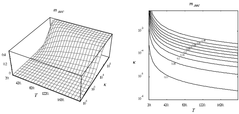
Figure 3: Mismatch between the initial and final states of a qubit in contact with an isotropic noise reservoir. The time scale starts at $t=20$ to match the encoding and decoding times in comparing this figure with the numerical results for the case of a qubit with error correction. This follows the storage scenario of Sect 3.2.1.

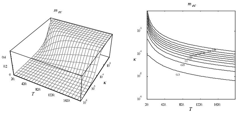
Figure 4: Mismatch between the initial and final states of a qubit with a five bit error correction code. The time scale starts at $t=20$ units to include the encoding and decoding times ($\Delta=10+10=20$). Each step (one or several gates) is effected in unit time, as indicated in Fig. 2.

A similar figure can be obtained by plotting the mismatch $m_{ec}$ of a qubit that has been encoded and later decoded. Instead of looking at the mismatch of a single qubit in contact with an isotropic noise reservoir for a time $T$, one encodes the qubit into five qubits ($10$ units of time), allows the five qubits to interact with the reservoir for $T-20$ units of time, and finally decodes and corrects the qubit ($10$ units of time). The resulting reduced density operator is used to compute $m_{ec}$ via (13). This mismatch, obtained by numerical simulation, is illustrated in Fig. 4.

Alternatively, we can use the results of Sect. 3 and estimate the mismatch by

$$m_{analytic}=\frac{1}{2}(1-s_{sc}(5)),$$ (44)

where $s_{sc}(n)$ is defined in (17). The agreement between this simple analytical model and the numerical simulations is very good, as illustrated in Fig. 5. The maximum discrepancy is of the order of 10 percent for our range of parameters.

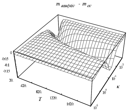
Figure 5: Difference between $m_{ec}$ and $m_{analytic}$, where $m_{ec}$ is the mismatch occuring in the numerical simulation and $m_{analytic}$ is the estimated mismatch from section 3. In both cases a single qubit is encoded into five and allowed to evolve in contact with a noisy environment, with noise occurring also during the encoding and the decoding phases. Time on the axis represents encoding and decoding time (i.e., $\Delta=10+10=20$ units of time) plus the time the encoded qubit is left interacting with the environment.

Consistent with the analysis developed in Sect. 3.2.3, one can identify in these numerical simulations a region of the $\kappa$-$T$ plane for which error correction is likely to help, despite noise occurring in the encoding and decoding stages. This can be clearly seen by looking (in analogy with Eq. 21) at the positive values of $\log(m_{nec}/m_{ec})$.

Another possible measure of the benefit of error correction is the difference $m_{ec}-m_{nec}$. Positive values of the difference indicate that error correction is worthwhile. However, this measure is of little use when both $m_{ec}$ and $m_{nec}$ go to zero, as their difference also vanishes. The $\log$ of the ratio does not have this drawback, and is therefore preferable as an indicator of where error correction is beneficial. The region of positive values of the $\log$ is represented by the shaded area in Fig. 6. One notices, as expected, that for small enough $\kappa$ and large $T$, error correction is desirable (since $\log(m_{nec}/m_{ec})>0\iff m_{ec}<m_{nec}$). For comparison, Fig. 7 shows the same quantity where the analytical expression $m_{analytic}$ of (44) has been used instead of $m_{ec}$.

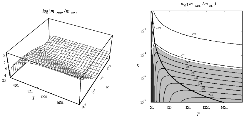
Figure 6: Surface and contour plots of $\log(m_{nec}/m_{ec})$, where $m_{ec}$ is generated numerically. The shaded area indicates values of $(\kappa,T)$ for which error correction is useful. This figure should be compared to Fig. 7. The thick line represents, for each given $\kappa$, the optimum time between the E and D stages (cf. Sect. 3.2.3, Eq. 22).

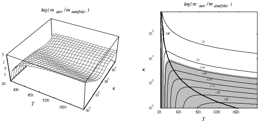
Figure 7: Same as Fig. 6, but here we plot $\log(m_{nec}/m_{analytic})$ instead of $\log(m_{nec}/m_{ec})$. The discrepancy between the numerical calculations and the analytical arguments is illustrated in Fig. 5.

An exactly similar set of calculations can be done for three bit codes in the case of delocalizing noise, and similar behavior was observed. In both the three bit and five bit cases, there is a section of the $\kappa$-$T$ plane where error correction remained beneficial even in the presence of noise during encoding and decoding; and for low values of the environmental interaction strength $\kappa$, there was an optimal time between error correction steps. This is consistent with the result obtained by Chuang and Yamamoto [13].

5 Conclusions

From both the analytical arguments and the numerical simulations, we see that error correction can prove worthwhile even in the presence of noise during encoding and decoding. For a given strength of the environmental coupling, there is an optimal rate at which error correction should be performed, and for a given time of storage there is an optimal number of error correction steps.

The simulations presented in this paper are among the first to treat both the execution of gates and the influence of the environment realistically, in the sense that the operation of gates takes a finite amount of time during which noise continues to act on the system. Moreover, models of the noise were used which correspond to common environmental effects in atomic and optical physics.

While the theory of error correction has moved rapidly, it is unlikely that circuits involving many qubits will be experimentally realized soon. Systems of a few qubits thus remain of great interest. Three-bit and five-bit error correction are among the first circuits that might be experimentally implemented, and hence our results should be of relevance to near-future experiments in this field.

We also have seen that quantum trajectories provide a practical technique for simulating systems with multiple qubits. This may prove particularly useful in treating systems with many qubits, where solving the full master equation is impractical due to the large size of the Hilbert space.

These simulations could be improved and extended in many ways. The Hamiltonians used to represent the gates were chosen for convenience rather than reflecting any particular physical system. It would be useful to get closer to the actual physics of proposed quantum computers, such as the linear ion trap of Cirac and Zoller [26]. In the same way, the coupling to the environment might differ for different gates. It would be straightforward to include these effects.

There are other interesting problems in quantum computation which might be studied by techniques like those of this paper. The recently proposed fault-tolerant error correction schemes are far more complicated than the ones treated in this paper. They would be beyond the reach of direct numerical simulation of the master equation with present computers, but may well prove amenable to a quantum trajectory approach.

Quantum computation still faces many hurdles before becoming reality. But it is far too early to say that the ingenuity of those working in the field is not sufficient to overcome them.

Acknowledgments

The authors acknowledge A. Ekert, N. Gisin, R. Laflamme, I.C. Percival and M. Plenio for useful conversations. We are grateful to Hewlett-Packard for use of computational resources. A.B. acknowledges the financial support of the Berrow’s fund at Lincoln College (Oxford) and of the Swiss National Science foundation. T.A.B. and R.S. acknowledge financial support from the UK EPSRC. This research was partially supported by the TMR Network Programme of the European Commission on the Physics of Quantum Information.

References

- [1] P. W. Shor, Proceedings of the 35th Annual Symposium on the Theory of Computer Science, ed. S. Goldwasser, IEEE Computer Society Press, Los Alamitos, CA, 124 (1994).
- [2] P. W. Shor, Phys. Rev. A 52, 2493 (1995).
- [3] A. M. Steane, Phys. Rev. Lett 77, 793 (1996).
- [4] A. M. Steane, “Multiple particle interference and quantum error correction,”, to appear in Proc. Roy. Soc. London A.
- [5] A. M. Steane, “Simple quantum error correcting codes,” quant-ph/9605021.
- [6] A. R. Calderbank and P. W. Shor, Phys. Rev. A. 54, 1098 (1996).
- [7] D. Gottesman, Phys. Rev. A 54, 1862 (1996).
- [8] A. R. Calderbank, E. M. Rains, P. W. Shor, and N. J. Sloane, “Quantum error correction and orthogonal geometry,” quant-ph/9605005.
- [9] R. Laflamme, C. Miquel, J. P. Paz, and W. H. Zurek, Phys. Rev. Lett. 77, 198 (1996).
- [10] C. H. Bennett, D. P. DiVincenzo, J. A. Smolin, and W. K. Wooters, Phys. Rev. A 54, 3824 (1996).
- [11] P. W. Shor, “Fault tolerant quantum computation”, quant-ph/9605011.
- [12] D. P. DiVincenzo and P. W. Shor Phys. Rev. Lett. 77, 3260 (1996).
- [13] I. L. Chuang and Y. Yamamoto, “The Persistent Qubit”, quant-ph/9604030.
- [14] U. Weiss, Quantum dissipative systems, Series in Modern Condensed Matter Physics Vol.2, (World Scientific Publishing, 1993).
- [15] G. Lindblad, Commun. Math. Phys. 48, 119 (1976).
- [16] Most of these papers are available from the e-print archive at http://xxx.lanl.gov.
- [17] S. L. Braunstein, “Quantum error correction of dephasing in 3 qubits”, quant-ph/9603024.
- [18] A. Barenco, C. H. Bennett, R. Cleve, D. P. DiVincenzo, N. Margolus, P. Shor, T. Sleator, J. Smolin, and H. Weinfurter, Phys. Rev. A 52, 3457 (1995).
- [19] L. Diósi, Phys. Lett. A 114, 451 (1986).
- [20] N. Gisin and I. C. Percival, J. Phys. A 25, 5677 (1992).
- [21] H. J. Carmichael, An Open Systems Approach to Quantum Optics, Lecture Notes in Physics m18, (Springer-Verlag, Berlin, 1993).
- [22] J. Dalibard, Y. Castin, and K. Mølmer, Phys. Rev. Lett. 68, 580 (1992).
- [23] C. W. Gardiner, A. S. Parkins, and P. Zoller, Phys. Rev. A 46, 4363 (1992).
- [24] J. K. Breslin, G. J. Milburn, and H. M. Wiseman, Phys. Rev. Lett. 74, 4827 (1995).
- [25] R. Schack and T. A. Brun, “A C++ library using quantum trajectories to solve quantum master equations”, to appear in Comp. Phys. Commun. The software is available from the authors or from http://galisteo.ma.rhbnc.ac.uk/applied/QSD.html.
- [26] J. I. Cirac and P. Zoller, Phys. Rev. Lett. 74, 4091 (1995).